optimization of neutral functional-differential inclusions

Optimization of Neutral Functional-Differential Inclusions

Elimhan N. Mahmudov & Dilara Mastaliyeva

Received: 19 June 2013 /Revised: 25 November 2013# Springer Science+Business Media New York 2014

Abstract A Bolza problem of optimal control theory with a varying time interval given byconvex, nonconvex functional-differential inclusions (PN), (PV) is considered. Our main goal isto derive sufficient optimality conditions for neutral functional-differential inclusions, whichcontain time delays in both state and velocity variables. Both state and endpoint constraints areinvolved. Presence of constraint conditions implies jump conditions for conjugate variable whichare typical for such problems. Sufficient conditions under the t1-transversality condition areproved incorporating the Euler–Lagrange- and Hamiltonian-type inclusions. As supplementaryproblems with discrete and discrete approximation inclusions (PD), (PDA) are considered andnecessary, and sufficient conditions are given. The basic concept of obtaining optimalityconditions is locally adjoint mappings and especially proved equivalence theorems. Further-more, the application of these results is demonstrated by solving some illustrative examples.

Keywords Discrete . Differential . Inclusion . Neutral . Hamiltonian . Locally adjointmultifunction . Transversality

AMS subject classifications 49K24 . 49K25 . 54C60

1 Introduction

This paper describes necessary and sufficient conditions for optimality in the followingoptimal control problems. At first, we consider the problem with neutral discrete inclusions:

PDð Þ minimize ∑t¼1

T

g xt; tð Þ ;subject to xtþ1∈Ft xt; xt−h; xt−hþ1ð Þ; t ¼ 0;…; T−1

xt ¼ ξt; t ¼ −h;−hþ 1;…; 0;xt ∈ Φt; t ¼ 1;…; T ;xT ∈ Q;

J Dyn Control SystDOI 10.1007/s10883-014-9215-x

E. N. Mahmudov (*)Industrial Engineering Department, Faculty of Management, Istanbul Technical University,34367 Macka-İstanbul, Turkeye-mail: [email protected]

E. N. Mahmudov :D. MastaliyevaInstitute of Cybernetics, Azerbaijan National Academy of Sciences, 9 B.Vahabzade str., AZ1141 Baku,Azerbaijan

where g(. , t):Rn→R1∪{+∞} is a function taking values on the extended line for all t = 1,…,T; Ft : R

3n →P (Rn) is a multifunction; ξt are fixed vectors (t = –h, …, 0); Q and Фt are somesets in Rn; and T, h are fixed natural numbers. Here, P (Rn) denotes the family of all subsets of

Rn. It is required to find a feasible trajectory {xt}t = −hT minimizing the sum∑

t¼1

tT

g xt; tð Þ . Theterm “neutral discrete inclusions” will become clearer in Section 2.

Our second problem is a Bolza problem with state constraints for functional-differentialinclusion of neutral type: choose an arc, which is an absolutely continuous function on [t0–h, t0)and [t0, t1] (t = t0 could be a point of discontinuity) to

minimize J x :ð Þ; t1½ � : ¼ φ x t1ð Þt1ð Þ þZt0

t1

g x tð Þ; tð Þdt;

PNð Þ subject to x� tð Þ ∈ Fðx tð Þ; x t−hð Þ; x� t−hð Þ; tÞa:e:t ∈ t0; t1½ �;x tð Þ ¼ ξ tð Þ;∀t∈ t0−h; t0½ Þh > 0;x tð Þ ∈Φ tð Þ ; ∀ t ∈ t0; t1½ � ;x t1ð Þ ∈ Q ;

where F (. , t) : R3n → P (Rn) is a multifunction for all fixed t ∈ [t0, t1]; the target set Q ⊂ Rn is aset of points x (t1);Ф:[t0, t1]→ P (Rn) is a multifunction; g, 8: Rn×[t0, t1]→ R1 ∪ {+∞}, ξ (.) isan absolutely continuous function on [t0−h,t0); t0 is fixed and t1 is generally free; and h>0 is aconstant delay. The integral in cost functional J is understood in means of Lebesgue.

It can be seen that such problems contain time delays not only in state variables but also invelocity variables. This makes the neutral-type problems essentially more complicated thandelay-differential inclusions. In particular, it is known that an analog of Pontryagin MaximumPrinciple does not generally hold for neutral systems, without convexity assumptions [9], andthis means that such problems are special to investigate.

The third problem is the same problem as (PN), but with the variable delay-differentialinclusion:

minimize J x :ð Þ; t1ð Þ½ � : φ x t1ð Þt1ð Þ þZt0

t1

g x tð Þ; tð Þdt;

PVð Þ subject to x: tð Þ∈F x tð Þ; x t−h tð Þð Þ; tð Þa:e:t ∈ t0; t1½ �;x tð Þ ¼ ξ tð Þ; t0−h t0ð Þ≤ t≤ t0;x tð Þ∈Φ tð Þ ; ∀ t ∈ t0; t1½ � ;x t1ð Þ ∈ Q ;

where F (. ,t) : R2n → P (Rn), h(⋅)is a differentiable function satisfying the inequalities h (t) >0,h′ (t)<1 and ξ (⋅) is absolutely continuous on t0−h(t0) ≤ t ≤ t0. We minimize the cost functionalJ over absolutely continuous functions x: [t0−h(t0),t1]→Rn satisfying the indicated delay-differential inclusion (PV) with initial condition x (t) = ξ (t), t0−h(t0) ≤ t ≤ t0 and state constrainton [t0, t1].

Optimal control problems with ordinary and partial differential inclusions consist one of theintensive developable areas in mathematical theory of optimal processes [1–4, 7, 8, 10, 15, 21,22, 24, 26, 27, 30–35]. More specifically, we deal with similar problems with both hereditaryand state constraints of Bolza type. Observe that such problems arise frequently not only inmechanics, aerospace engineering, management science, and economies but also in problems

Elimhan N. Mahmudov and Dilara Mastaliyeva

of automatic control, autovibiration, burnings in rocket motors, biophysics, and so on [6, 9,11–14, 17, 24, 28, 29, 33]. Moreover, neutral systems have some similarities with the so-calledhybrid and differential-algebraic equations that are important in engineering controlapplication.

Optimization of differential inclusions with state constraints is not easy to solve; there aredifferent approaches and various results in this area using one or another tool in non-smoothanalysis, we refer the reader to [6, 8, 10, 15, 18, 19, 23, 26, 27, 30, 32, 34, 35]. The matter is thatin these problems the presence of state constraints on an optimal control trajectory manifestsitself in the sufficient conditions by producing discontinuities in the corresponding adjoint arc;we show that one of the adjoint variables has jumps which are typical for such problems, andamong sufficient conditions, there appears a condition of jumps where the number of jumppoints may be countable. Most of the appropriate results are obtained for the Mayer problem(g = 0) and fixed time interval; see [15, 16, 20] and their references. Time optimal controlproblem (8 = 0, g = 1) is considered in [3]. So our aim is to establish well-verifiable sufficientconditions for optimality for functional and delay-differential inclusions with state constraintsand free time. Our conditions are more precise than any previously published ones since theyinvolve useful forms of the Weierstrass–Pontryagin condition and the Euler–Lagrange-typeadjoint inclusions [3, 4, 29, 34]. As suggested in our previous papers [18–22], we expect allof these improvements to serve for the future developments of optimal control theory withfunctional-differential inclusions. The rest of the paper is organized as follows.

In Section 2 under the Hypothesis (H1) consisting of more general assumptions we provethe necessary and sufficient conditions for the defined neutral-type discrete (PD) and discreteapproximation (PDA) inclusions. Observe that these results are based on the new apparatus oflocally adjoint multifunction (LAM). Another definition of the LAM was introduced byPshenychnyi [29] and applied in papers of Mahmudov [18–20]. Besides, the similar notionis given by Mordukhovich [24] and is called coderivative of multifunctions at a point. The useof LAM and convex upper approximation (CUA) for nonconvex functions and locally tents[29] are very suitable to get the optimality conditions for posed problems. For problems withconvex structure (PD), (PN), there are other adjoint inclusions formulated in terms of LAM andtherefore more subtle optimality conditions. In the area of different convex and nonconvexapproximations of functions and sets, the reader can also consult Clarke [5, 7], Demyanov [8],Mordukhovich [24], Pshenychnyi [29], Rockafellar [15], etc. The second part of Section 2 isdevoted to the limiting procedure in discrete approximation problem that allows us to have theresults concerning sufficient conditions for functional-differential inclusion.

In Section 3 the basic idea is to pass to the formal limit in the necessary conditions forproblem (PDA) to establish sufficient conditions for optimality of the original nonconvexneutral-type continuous time problem (PN). Therefore as a result of the monotonicity conditionof Bolza cost functional on t and t1-transversality condition, sufficient conditions for optimalityare derived. Note that transition to the problem (PDA) requires special equivalence Theorems2.2 and 2.3 of a LAM connecting the main results of (PD) and (PDA) problems. We emphasizethat the key to our success is the formulation of the equivalence theorems.

The proposed finite difference methods and the results obtained can be used for numericalsolutions of infinite-dimensional problems. But our main interest here is to use finite differenceapproximations and construct sufficient optimality conditions for problems (PN) and (PV). Inparticular, for convex problem of neutral type (PN) with fixed time interval, the sufficientconditions are proved (Theorem 3.2).

In the reviewed results, the arising adjoint inclusions are stated in the Euler–Lagrange formand this effort culminates in Theorems 3.1 and 3.2. For a different type of problems connectedwith neutral type functional and delay-differential inclusions, we can advise the reader the


papers of Mordukhovich and Wang [25] and Medhin [26]. Note that, in the paper [25], thevalue convergence of discrete approximations is established as well as the strong convergencesof optimal arcs in the classical Sobolev space W1,2 .

Finally, the problem of optimal control (PN) with the functional-differential inclusionslinear in velocities involving neutral-type operator given in the Hale form [10, 25, 26]:ddt x tð Þ−Ax t−hð Þ½ �∈F x tð Þ; x t−hð Þ; tð Þ is considered (Theorem 3.3). Note to this end that trajec-tories x(⋅) being continuous (except may be the point t0) of Hale form differential inclusion aregenerally discontinuous on [t0−h, t1] while their linear combinations as result of Hale formbehave nicely on [t0, t1]. In the non-delayed case withA≠0, the obtained problem correspondingto implicit differential inclusions represent substantial interest, too.

Section 4 deals with the complicated problem with differential inclusion (PV), whichinvolve the variable delay. For such nonconvex problem, the sufficient condition is formulated.The considered simple examples show that the results obtained coincides with the results ofclassical optimal control theory [9, 24, 28].

Let (x1, x2) be a pair of elements x1, x2 ∈ Rn, and <x1, x2> be their inner product. Amultifunction F : R3n →P(Rn ) is convex if its graph gph F = {(x1, x2, x3, y) : y ∈ F (x1, x2, x3)}is a convex subset of R4n. It is convex-valued if F(x) is a convex set for each x=(x1, x2, x3) ∈dom F = {x : F (x) ≠ Ø}. F is closed if gph F is a closed set in R4n. Let us denote

H x; y�ð Þ ¼ supy

<y; y�>: y ∈ F xð Þf g; y� ∈ Rn;

F x; y�ð Þ ¼ y ∈ F xð Þ :<y; y�>¼ H x; y�ð Þf g:

For convex F,we let H (x, y*)=−∞, when F (x) = ∅. According to[24], we recall thefunction H the Hamiltonian and the set F (x, y*) argmaximum set.

Let riA be the relative interior of a set A ⊂ Rn, i.e., the set of interior points of Awith respectto its linear hull LinA.

The cone of tangent directions KA(x0), x0 ∈A is called a local tent [29] if for each x0 ∈ ri KA

(x0) there exists a convex cone K ⊆ KA (x0) and a continuous mapping Ψ (x ) defined in aneighborhood of the origin such that

(1) x0 ∈ ri K; Lin K ¼ Lin KA x0ð Þ;(2) Ψ x

� �¼ xþ r x

� �; x�� −1r x

� �→0 as x→0;

(3) x0 þ Ψ xð Þ ∈ A; x ∈ K ∩ Sε 0ð Þ for some ε > 0, where Sε (0) is the ball of radius ε andwith center of origin.

The function h (. , x) is called a CUA of a function g (⋅) : Rn → R1 ∪ {±∞} at every fixedpoint x ∈ domg = {x: |g (x)| < +∞} if

h x; xð Þ ≥ Ω x; xð Þ for all x ≠ 0 ; where

Ω x; xð Þ ¼ supr :ð Þ

limλ↓0

supg xþ λxþ r λð Þ−g xð Þð Þ

λ

Here, the exterior supremum is taken on all r(.) such that λ−1r (λ)→ 0, where λ ↓ 0. h (. , x) is aconvex closed (lower semicontinuous) positive homogeneous function. Further, the set


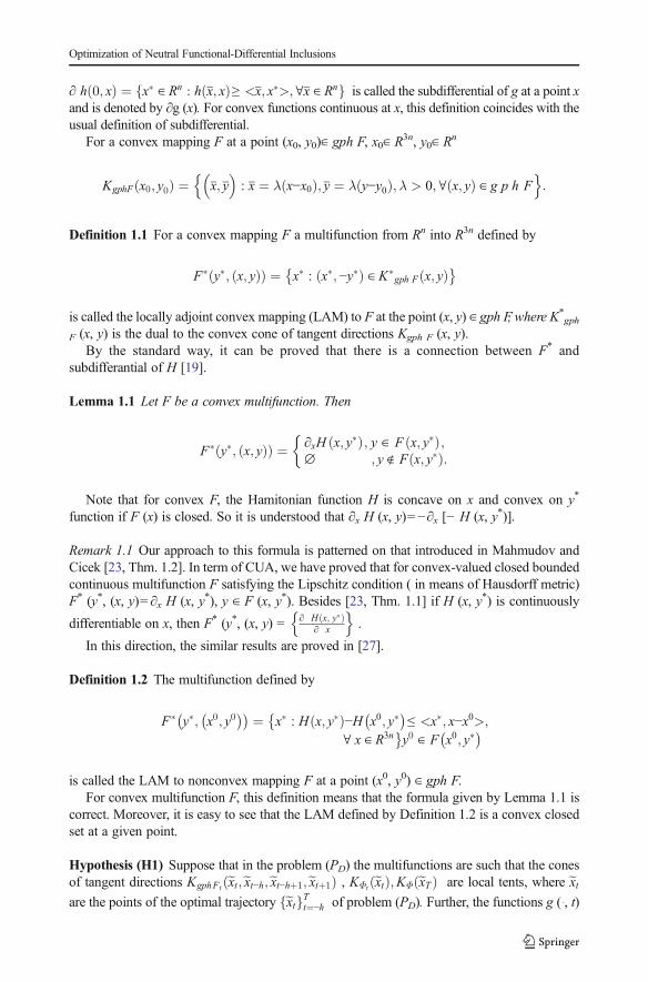
∂ h 0; xð Þ ¼ x� ∈ Rn : h x; xð Þ≥ <x; x�>;∀x ∈ Rnf g is called the subdifferential of g at a point xand is denoted by ∂g (x). For convex functions continuous at x, this definition coincides with theusual definition of subdifferential.

For a convex mapping F at a point (x0, y0)∈ gph F, x0∈ R3n, y0∈ Rn

KgphF x0; y0ð Þ ¼ x; y� �

: x ¼ λ x−x0ð Þ; y ¼ λ y−y0ð Þ;λ > 0;∀ x; yð Þ ∈ g p h Fn o

:

Definition 1.1 For a convex mapping F a multifunction from Rn into R3n defined by

F� y�; x; yð Þð Þ ¼ x� : x�;−y�ð Þ ∈ K�gph F x; yð Þ� �

is called the locally adjoint convex mapping (LAM) to F at the point (x, y) ∈ gph F, where K*gph

F (x, y) is the dual to the convex cone of tangent directions Kgph F (x, y).By the standard way, it can be proved that there is a connection between F* and

subdifferantial of H [19].

Lemma 1.1 Let F be a convex multifunction. Then

F� y�; x; yð Þð Þ ¼ ∂xH x; y�ð Þ; y ∈ F x; y�ð Þ;∅ ; y ∉ F x; y�ð Þ:

�

Note that for convex F, the Hamitonian function H is concave on x and convex on y*

function if F (x) is closed. So it is understood that ∂x H (x, y)=−∂x [− H (x, y*)].

Remark 1.1 Our approach to this formula is patterned on that introduced in Mahmudov andCicek [23, Thm. 1.2]. In term of CUA, we have proved that for convex-valued closed boundedcontinuous multifunction F satisfying the Lipschitz condition ( in means of Hausdorff metric)F* (y*, (x, y)=∂x H (x, y*), y ∈ F (x, y*). Besides [23, Thm. 1.1] if H (x, y*) is continuously

differentiable on x, then F* (y*, (x, y) = ∂ H x; y�ð Þ∂ x

n o.

In this direction, the similar results are proved in [27].

Definition 1.2 The multifunction defined by

F� y�; x0; y0� � ¼ x� : H x; y�ð Þ−H x0; y�

� ≤ <x�; x−x0>

�;

∀ x ∈ R3n�y0 ∈ F x0; y�

� is called the LAM to nonconvex mapping F at a point (x0, y0) ∈ gph F.

For convex multifunction F, this definition means that the formula given by Lemma 1.1 iscorrect. Moreover, it is easy to see that the LAM defined by Definition 1.2 is a convex closedset at a given point.

Hypothesis (H1) Suppose that in the problem (PD) the multifunctions are such that the conesof tangent directions KgphFt ext;ext−h;ext−hþ1;extþ1ð Þ , KΦt extð Þ;KΦ exTð Þ are local tents, where extare the points of the optimal trajectory extf gTt¼−h of problem (PD). Further, the functions g ( , t)


admit a CUA h x;extð Þ of the points ext that is continuous with respect to x and consequently∂ g ext; tð Þ ¼ ∂ ht 0;extð Þ is defined.

Hypothesis (H2) Let the problem (PD) be convex, i.e., involved functions, multifunction, andsets are convex and {xt

0}t = −hT be a feasible trajectory. Then suppose implementation either of

the two following conditions:

(a) x0t ; x0t−h; x

0t−hþ1; x

0tþ1

� ∈ ri gph Ft;t ¼ 0;…; T−1;

x0t ∈ ri Φt ∩ domg :; tð Þ; t ¼ 1;…; T ; x0T ∈ ri Q;

(b) x0t ; x0t−h; x

0t−hþ1; x

0tþ1

� ∈ i n t gph Ft; t ¼ 0;…; T−1; x0t ∈ int Φt; t ¼ 1; …; T ;

x0T ∈ Q and g ⋅; tð Þ are continuous at a point x0t :

2 Optimization of Neutral Discrete Inclusions (PD)

Theorem 2.1 Assume Hypothesis (H1) for the neutral type nonconvex problem (PD). Then for

the optimality of trajectory extf gTt¼−h , it is necessary that there exist a number λ∈{0,1} andvectors x*, xt

*, ηt*, φt

*, t = 0,1, …, T, simultaneously not all equal to zero, such that

(i) x�t −η�tþh−φ

�tþh−1; η

�t ;φ

�t

� ∈ F�

t x�tþ1~xt;~xt−h;~xt−hþ1;~xtþ1ð Þ�

− λ ∂xg ~xt; tð Þ−K�Φt

~xtð Þn o

� 0f g � 0f g; t ¼ 0;…; T−1−h;λ ∂x ~x0; 0ð Þ; K�

Φ0

~x0ð Þ ¼ 0;

(ii) x�t ; η�t;φ

�t

� ∈ F�

t x�tþ1~xt;~xt−h;~xt−hþ1;~xtþ1ð Þ�

− λ ∂xg ~xt;t�

−K�Φt

~xtð Þn o

� 0f g � 0f g; t ¼ T−h; …; T−1;x�−x�T ∈ λ ∂x g ~xT ; Tð Þ−K�

ΦT

~xTð Þ; x� ∈ K�Q~xTð Þ; η�T ¼ 0; φ�

T ¼ 0:

Proof Let us introduce the vector w=(x−h, x−h+1, …, x0, …, xT) ∈ Rn(h+1+T ) and define in thespace Rn(h+1+T ) the following sets:

Mt ¼ w : xt; xt−h; ; xt−hþ1; ; xtþ1ð Þ ∈ gph Ftf g; t ¼ 0;…; T−1;N ¼ w : xt ¼ ξt; t ¼ −h;−hþ 1;…; 0f g:Pt ¼ w : xt ∈ Φt; t ¼ 1;…; Tf g; MT ¼ w : xT ∈ Qf g:

Obviously, the problem (PD) is equivalent to the following problem:

minimize g wð Þ ¼Xt¼1

T

g xt; tð Þ;

subject to w ∈ N ∩ ∩t¼1

T

Mt

!∩ ∩

t¼1

T

Pt

!:

ð2:1Þ


In order to formulate the necessary and sufficient conditions [5, 14, 24, 29] for problem(2.1), we use the dual cones (see [31])

K�Mt

wð Þ ¼ w�f : x�t ; x�t−h; x�t−hþ1; x�tþ1

� ∈ K�

gphFtxt; xt−h; xt−hþ1; xtþ1

� ;

x�k ¼ 0; k ≠ t; t−h; t−hþ 1; t þ 1g ;w� ¼ x�−h;…; x�0;…; x�T

� ∈ Rn hþ1þTð Þ;

K�MT

wð Þ ¼ w� : x�T ; ∈ K�Q xTð Þ; x�t ¼ 0; t < T

n o;

K�Pt

wð Þ ¼ w� : x�t ; ∈ K�Φt

xtð Þ; x�k ¼ 0; k ≠ tn o

; t ¼ 1;…; T ;

K�N wð Þ ¼ w� : x�t ¼ 0; t ¼ −h;−hþ 1;…; 0

� �:

Then on the above-mentioned minimization theorems, there are the vectors

w� tð Þ ∈ K�Mt

~wð Þ; t ¼ 0;…; T ;w�h ∈ K�

N~wð Þ; w� tð Þ ∈ K�

Pt

~wð Þ; t ¼ 1; …; T ;~w ¼ ~x−h;~x−hþ1;…;~xTð Þ;~xt ¼ ξt; t ¼ −h;…; 0 ~x−h

and number λ ∈ {0, 1}, so that

λw�0 ¼ w�

h þXt¼0

T

w* tð Þ þXt¼1

T

w�tð Þ;w�

0 ∈ ∂wgðewÞ ð2:2Þ

Now, rewriting (2.2) in component wise form, we have

λx�t0 ¼ x�t tð Þ þ x�t t−1ð Þ þ x�t t þ hð Þ þ x�t t þ h−1ð Þ þ x�t tð Þ; t ¼ 0; :; T−1−h; ð2:3Þ

λx�t0 ¼ x�t tð Þ þ x�t t−1ð Þ þ x�t tð Þ; t ¼ T−h;…; T−1; ð2:4Þ

λx�T0 ¼ x�T T−1ð Þ þ x�T Tð Þ þ x�T Tð Þ; ð2:5Þ

x�t−h tð Þ ¼ 0; x�t−hþ1 tð Þ ¼ 0; t ¼ T ; x �t0 ∈ ∂xg ext; t� �

; t ¼ 1;…; T : ð2:6Þ

where x�t tð Þ is a component of the vector w� tð Þ .Then by Definition 1.1 of LAM, it follows from relations (2.3), (2.4) that

λx�t0−x�t t þ hð Þ−x�t t þ h−1ð Þ−x�t t−1ð Þ−x�t tð Þ; x�t−h tð Þ; x�t−hþ1 tð Þ�

∈ F�t −x�tþ1 tð Þ; ~xt;~xt−h;~xt−hþ1;~xtþ1ð Þ�

; t ¼ 0 ; … ; T −1−h ; ð2:7Þ

λx�t0−x�t t−1ð Þ−x�t tð Þ; x�t−h tð Þ; x�t−hþ1 tð Þ�

∈ F�t −x�tþ1 tð Þ; ~xt;~xt−h;~xt−hþ1;~xtþ1ð Þ�

; t ¼ T−h;…; T−1: ð2:8Þ

At last, denoting xt*≡−xt* (t−1), ηt*≡xt−h* (t), 8t

*≡xt−h+1* (t), x* = xT* (T ) and taking into

account (2.5), (2.6) and (2.7), (2.8), we obtain the conditions (i), (ii), and (iii).


Remark 2.1 For convex problem (PD) under the Hypothesis (H2), the conditions (i)–(iii) are

also sufficient for optimality of the trajectory extf gTt¼−h . It occurs because the representation(2.2) holds with the parameter = 1.

Remark 2.2 Let Ft , t=0, …, T−1 be upper semicontinuous multifunctions, Ф t, Q be closedsets, and g (., t) be a lower semicontinuous for any fixed t. Then the posed problem (PD) can bereduced to the minimization of lower semicontinuous function on compact (see [31]) set, and

so under the existence of some feasible trajectory extf gTt¼−h , the optimal solution exists.Let L be any natural number, t1 be a fixed number and δ ¼ h

L . Then, we define the pointst0+kδ, k = −L…, T, t0+(T+1)δ = t1, where the natural T satisfies the inequality t0+Tδ≤t1<t0+(T+1)δ with respect to the problem (PN), we associate the discrete approximating problem:

minimize Jδ

x tð Þð Þ :¼ φ x tð Þð Þ þX

t¼t0;t0þδ;…;t1−δδg x tð Þ; tð Þ

ðPDAÞ subject toΔx tð Þ ∈ F x tð Þ; x t−hð Þ;Δx t−hð Þ; tð Þ; t ¼ t0; t0 þ δ;…; t1−δ;x tð Þ ¼ ξ tð Þ; t ¼ t0−h; t0−hþ δ;…; to−δ;x tð Þ ∈ Ф tð Þ; t ¼ t0; t0 þ δ;…; t1;x t1ð Þ ∈ Q;

where

Δx tð Þ ¼ x t þ δð Þ−x tð Þδ

:

In order to formulate the sufficient condition for the continuous problem (PN), it is requiredto define the form of the adjoint inclusion for it. With this aim, we use discrete inclusion (2.9)and Theorem 2.1. Let us write (2.9) in the so-called neutral discrete fo

x t þ δð Þ ∈ Q x tð Þ; x t−hð Þ; x t−hþ δð Þ; t;ð Þ ð2:10Þ

Q x1; x2; x3; tð Þ ¼ x1 þ δ F x1; x2;x3−x2δ

; t� �

: ð2:11Þ

Then, it follows from Theorem 2.1 that the adjoint inclusion for the discrete approximatingproblem with discrete inclusion (2.10) must be expressed in terms of LAM Q*. That is why themain arising problem is the connection between LAM Q* and F*. This connection is ofprincipal importance for the proposal method in our work.

Remark 2.3 Comparing discrete approximation inclusions (2.10) with discrete inclusions inthe problem (PD), we see that the name “neutral” is justified.

Theorem 2.2 Let Q(., t) be defined by (2.11)multifunction andKgph Q(.,t) (x1, x2, x3,y), (x1, x2, x3, y)∈ gph Q (., t) be a local tent. Then

KgphF :;tð Þ x1; x2;x3−x2δ

;y−x1δ

� �is a local tent to gph F(., t) and the following inclusions are equivalent:

(1) ; x1; x2; x3; yð Þ ∈ Kgph Q :;tð Þ x1; x2; x3; yð Þ;(2) x1; x2;

x3−x2δ ; y−x1

δ

� �∈ KgphF :;tð Þ x1; x2;

x3−x2δ ; y−x1

δ

� :

(2.9)


Proof It follows from the definition of the local tent that for functions ri zð Þ; i ¼ 0; 1; 2; 3;

z ¼ x1; x2; x3; y�

possessing the property ri zð Þ zk k−1→ 0; z→0 is valid

yþ yþ ro zð Þ ∈ x1 þ x1 þ r1 zð ÞþδF x1 þ x1 þ r1 zð Þ; x2 þ x2 þ r2 zð Þ; x3 þ x3 þ r3 zð Þ−x2−x2−r2 zð Þ

δ; t

�

for small z ∈ K ⊆ ri Kgph Q :;tð Þ. Transforming this inclusion, we have

y−x1δ

þ y−x1δ

þ r0 zð Þ−r1 zð Þδ

∈Fðx1 þ x1 þ r1 zð Þ; x2 þ x2 þ r2 zð Þ; x3 þ x3δ

þ x3−x2δ

þ r3 zð Þ−r2 zð Þδ

; tÞ

Then, it is clear that the inclusion (2) is valid. By going to the reverse direction, we obtaincorrectness for inclusion (1).

Theorem 2.3 Let KgphQ(.,t) be a local tent for multifunction Q (., t). Then the followinginclusions are equivalent:

(1) x�1; x�2; x

�3

� ∈ Q� y�; x1; x2; x3; yð Þ; tð Þ;

(2) x�1−y�

δ;x�2 þ x�3

δ; x�3

�∈F� y�; x1; x2;

x3−x2δ

;y−x1δ

� �; tÞ

� �:

Proof Let us prove (1) ⇒ (2). On the definition of LAM, the relation (1) means that

x1; x�1

� þ x2; x�2

� þ x3; x�3

� − y; y�h i≥0;

x1; x2; x3; yð Þ ∈ Kgph Q :;tð Þ x1; x2; x3; yð Þ ð2:12Þ

Due to Theorem 2.2, the inequality (2.12) can be rewritten in the form

x1;ψ�1

D Eþ x2;ψ

�2

D Eþ x3−x2

δ;ψ�

3

* +−

y − x1δ

;ψ�* +

≥0 ð2:13Þ

where ψ1*, ψ2

*, and ψ* are to be determined. Comparing (2.12) and (2.13), it is not hardto see that

ψ� ¼ y�;ψ�1 ¼

x�1−y�

δ;ψ�

2 ¼x�2 þ x�3

δ:

By analogy, the inverse transition (2)⇒ (1) can be shown. The proof of theorem is completed.


Now, let us return to the discrete approximation problem (PDA) with inclusion (2.10). Theconditions (i)–(iii) of Theorem 2.1 gain the following form:

x� tð Þ–η� t þ hð Þ–φ� t þ h−δð Þ; η� tð Þ;φ� tð Þð Þ∈Q� x� t þ δð Þ; ex tð Þ;ex t−hð Þ;ex t−hþ δð Þ;ex t þ δð Þ

� �t

� �− λδ ∂xg ex tð Þ; t

� �−K�

Φ tð Þ ex tð Þ� �n o

� 0f g � 0f g;λ ¼ λδ ∈ 0; 1f g

∂xg ex t0ð Þ; t0;¼ 0;K�Φ t0ð Þ ex t0ð Þ� �

¼ 0; t ¼ t0; t0 þ δ;…; t1−h−δ;�

x� tð Þ; η� tð Þ;φ� tð Þð Þ ∈Q� x� t þ δð Þ; ex tð Þ� �ex t−hð Þ;ex t−hþ δð Þ;ex t þ δð Þ

� �; tÞ

ð2:14Þ

− λδ ∂xg ~x tð Þ; tð Þ−K�Φ tð Þ ~x tð Þð Þ

n o� 0f g � 0f g; t ¼ t1−h;…; t1−δ;

x�−x� t1ð Þ ∈ λδ ∂xφ ~xð t1ð Þ−K�Φ t1ð Þ ~x t1ð Þð Þ; x� ∈ K�

Q~x t1ð Þð Þ; ð2:15Þ

η� t1ð Þ ¼ 0;φ� t1ð Þ ¼ 0: ð2:16ÞThen by using the Theorem 2.3, it is easy to see that the conditions (2.14), (2.15) can be

expressed as follows, respectively:

−Δx� tð Þ−η� t þ hð Þ−φ� t þ hð Þ

δþ Δφ� t þ h−δð Þ; η

� tð Þ−φ� tð Þδ

; φ� tð Þ �

∈F� x� t þ δð Þ;~x tð Þ;~x t−hð Þ;Δ~x t−hð Þ;Δ~x tð ÞÞ; tð Þ− λδ∂xg ~x tð Þ; tð Þ−K�

Φ tð Þ ~x tð Þð Þn o

� 0f g � 0f g ;t ¼ t0; t0 þ δ;…; t1−δ−h; (2.17)

−Δx� tð Þ; η� tð Þ þ φ� tð Þδ

; φ� tð Þ �

∈F� x� t þ δð Þ; ~x tð Þ;~x t−hð Þ;Δ~x t−hð Þ;Δ~x tð Þð Þ; tð Þ

− λδ∂x ~x tð Þ; tð Þ−K�Φ tð Þ ~xð tð Þ

n o� 0f g � 0f g; t ¼ t1−h;…; t1−δ: ð2:18Þ

Let us summarize the obtained result.

Corollary 2.1 Let assumptions (H1) for the difference neutral type nonconvex problem (PDA)hold. Then for the optimality of the trajectory ex tð Þf gt1t¼−h , it is necessary that there exists anumber λδ ∈ {0,1} and grid functions x*(t), η*(t), φ*(t), t = t0, t0+δ,…,t1 simultaneously not allequal to zero satisfying the conditions (2.16)–(2.18). Moreover, let us assume that φ(.) andg(.,t) are convex proper functions and continuous at the points of some feasible grid trajectory

x0 tð Þ� �t1t¼−h . Then under the Hypothesis (H2), the conditions (2.16)–(2.18) are also sufficient

for optimality in convex problem (PDA).

It should be noted that setting λδ = 1 and denoting the expression η� tð Þþφ� tð Þδ by ζ*(t) and

passing to the formal limit in (2.17), (2.18) when L→∞ and consequently δ→0 we have

−x:� tð Þ−ζ� t þ hð Þ þ φ:�

t þ hð Þ; ζ� tð Þ;φ� tð Þ� �∈F� x� tð Þ; ~x tð Þ;~x t−hð Þ; �~x t−hð Þ; �~x tð Þ�

; t�

− ∂x g ~x tð Þ; tð Þ−K�Φ tð Þ ~x tð Þð

n o� 0f g � 0f g; t ∈ t0; t1−h½ Þ;

ð2:19Þ


−x � tð Þ; ζ� tð Þ;φ� tð Þð Þ ∈ F� x� tð Þ; ~x tð Þ;ex t−hð Þ; �~x t−hð Þ; �~x tð Þ� �

; t� �

− ∂x g ~x tð Þ; tð Þ−K�Φ tð Þ ~x tð Þð

n o� 0f g � 0f g; t ∈ t1−h; t1½ �:

ð2:20Þ

Below(Theorem 3.2), we will be sure that the differential inclusions (2.19), (2.20) are justthe needed conjugate inclusions for convex problem (PN) with fixed time interval [t0, t1].

3 Sufficient Condition for the Optimality of the Neutral Functional-DifferentialInclusions

Let ex (t), t∈ [t0−h, t1], ex (t)=ξ(t), t∈[t0−h, t0] be some feasible solution of the nonconvexproblem (PN). First let us construct the adjoint differential inclusion for adjoint variables {x

*(.),ζ*(.), φ*(.)}. Of course for this we use the approximating method demonstrated above inSection 2. Thus, the adjoint inclusions expressed in terms of LAM consist of the following:

(a) −x � tð Þ−ζ� t þ hð Þ þ φ � t þ hð Þ; ζ� tð Þ;φ� tð Þð Þ∈F� x� tð Þ; ~x tð Þ;~x t−hð Þ; �~x t−hð Þ; �~x tð Þ� ; t

� a:e:t ∈ t0; t1−h½ Þ;

(b) −x � tð Þ; ζ� tð Þ;φ� tð Þð Þ∈F� x� tð Þ; ~x tð Þ;~x t−hð Þ; �~x t−hð Þ; �~x tð Þ� ; t

� a:e:t ∈ t1−h; t1½ �;φ� t1ð Þ ¼ 0;

(c)�~x tð Þ ∈ F ex tð Þ;~x t−hð Þ; �~x t−hð Þ; x� tð Þ; t

� �a:e:t ∈ t0; t1½ �:

which should be fulfilled for all x ∈ Φ (t).Here, a feasible solution is understood to be the triplet {x*(.), ζ*(.), φ*(.)} satisfying the

conditions (a), (b) almost everywhere such that ζ*(.), φ*(.) are absolutely continuous and x*(.)may be represented as a sum of the absolutely continuous function and a function of jumps.Let us denote the points of jumps and the values of jumps of x*(.) by τi, t0 < τi < t1 and xi

*=x*

(τi+0)−x* (τi−0), i =1, 2, …, respectively.Let us denote for a set S ⊂ Rn

Ms x�ð Þ ¼ sup x�; yh i

y ∈ S

and let the feasible solutionex (t) is a so-called the t1-transversal on the setQ, i.e., the followingcondition holds for every t ∈ [t0, t1]:

− x� tð Þ;~x tð Þh i > MQ∩Φ tð Þ −x� tð Þð Þ; t0≤ t < t1:

Obviously, for every t ∈ [t0, t1), the point ex tð Þ∉ Q ∩ Ф(t) and so ex tð Þ∉ Q. In otherwords, the t1-transversality condition guarantees that the point ex tð Þ belongs to the setQ only at the moment t = t1. Furthermore, assume that the Bolza cost functionalJ[x(�), t] is monotone increasing with respect to argument t, that is, the inequalityJ[(x(�), θ1]<J [x(�), θ2] holds for any θ1, θ2 ∈ [t0, t1] (θ1 < θ2) and for any feasible arc x(�) of thedifferential inclusion in problem (PN).

Remark 3.1 The monotonicity condition of Bolza cost functional J[x(�), t] on t for any feasiblearc x(�) is satisfied for a wide class of problems. For example, it is fulfilled for time optimal


control problems (φ≡0, g≡1), for problems with quadratic cost functional, for Lagrange(φ(x, t)≡0) problems with nonnegative integrand g and so on.

Finally, we can formulate sufficient conditions for optimality in the form of the followingtheorem.

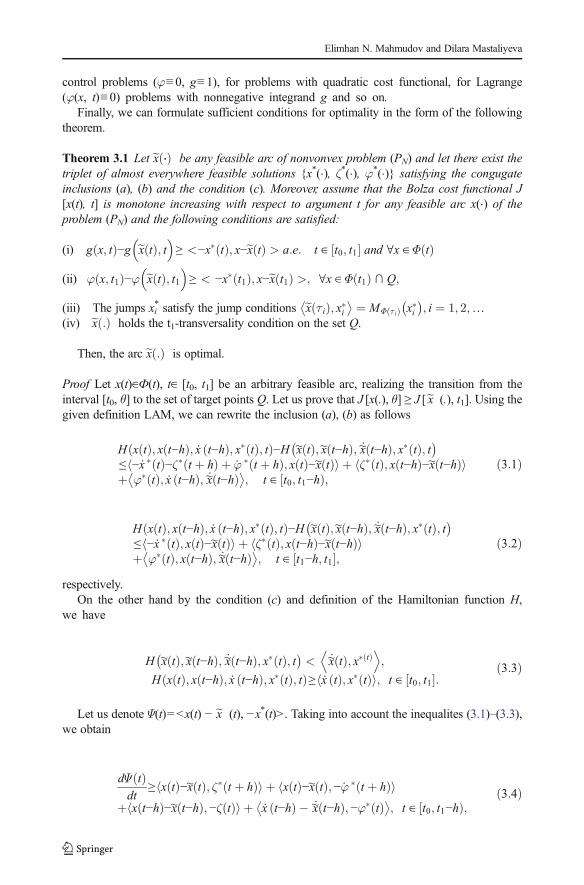
Theorem 3.1 Let ex ⋅ð Þ be any feasible arc of nonvonvex problem (PN) and let there exist thetriplet of almost everywhere feasible solutions {x*(�), ζ*(�), φ*(�)} satisfying the congugateinclusions (a), (b) and the condition (c). Moreover, assume that the Bolza cost functional J[x(t), t] is monotone increasing with respect to argument t for any feasible arc x(�) of theproblem (PN) and the following conditions are satisfied:

(i) g x; tð Þ−g ex tð Þ; t� �

≥ <−x� tð Þ; x−ex tð Þ > a:e: t ∈ t0; t1½ � and ∀x ∈ Φ tð Þ

(ii) φ x; t1ð Þ−φ ex tð Þ; t1� �

≥ < −x� t1ð Þ; x−ex t1ð Þ >; ∀x ∈ Φ t1ð Þ ∩ Q;

(iii) The jumps xi* satisfy the jump conditions ex τ ið Þ; x�i

� ¼ MΦ τ ið Þ x�i�

; i ¼ 1; 2;…(iv) ex :ð Þ holds the t1-transversality condition on the set Q.

Then, the arc ex :ð Þ is optimal.

Proof Let x(t)∈Ф(t), t∈ [t0, t1] be an arbitrary feasible arc, realizing the transition from theinterval [t0, θ] to the set of target points Q. Let us prove that J [x(.), θ] ≥ J [ex (.), t1]. Using thegiven definition LAM, we can rewrite the inclusion (a), (b) as follows

H x tð Þ; x t−hð Þ; x t−hð Þ; x� tð Þ; tð Þ−H ~x tð Þ;~x t−hð Þ; �~x t−hð Þ; x� tð Þ; t� ≤ −x � tð Þ−ζ� t þ hð Þ þ φ � t þ hð Þ; x tð Þ−~x tð Þh i þ ζ� tð Þ; x t−hð Þ−~x t−hð Þh iþ φ� tð Þ; x t−hð Þ; �~x t−hð Þ�

; t ∈ t0; t1−h½ Þ;ð3:1Þ

H x tð Þ; x t−hð Þ; x t−hð Þ; x� tð Þ; tð Þ−H ~x tð Þ;~x t−hð Þ; �~x t−hð Þ; x� tð Þ; t� ≤ −x � tð Þ; x tð Þ−~x tð Þh i þ ζ� tð Þ; x t−hð Þ−~x t−hð Þh iþ φ� tð Þ; x t−hð Þ; �~x t−hð Þ�

; t ∈ t1−h; t1½ �;ð3:2Þ

respectively.On the other hand by the condition (c) and definition of the Hamiltonian function H,

we have

H ~x tð Þ;~x t−hð Þ; �~x t−hð Þ; x� tð Þ; t� <

�~x tð Þ; x� tð ÞD E

;

H x tð Þ; x t−hð Þ; x t−hð Þ; x� tð Þ; tð Þ≥ x tð Þ; x� tð Þh i; t ∈ t0; t1½ �:ð3:3Þ

Let us denote Ψ(t)=<x(t) − ex (t), −x*(t)>. Taking into account the inequalites (3.1)–(3.3),we obtain

dΨ tð Þdt

≥ x tð Þ−~x tð Þ; ζ� t þ hð Þh i þ x tð Þ−~x tð Þ;−φ � t þ hð Þh iþ x t−hð Þ−~x t−hð Þ;−ζ tð Þh i þ x t−hð Þ � �~x t−hð Þ;−φ� tð Þ�

; t ∈ t0; t1−h½ Þ;ð3:4Þ


dΨ tð Þdt

≥ x t−hð Þ−ex t−hð Þ; ζ� tð ÞD E

þ x t−hð Þ− �~x t−hð Þ;−φ� tð Þ� t ∈ t1−h; t1½ �: ð3:5Þ

Now, integrating both sides of the inequalites (3.4), (3.5) on the intervals [t0, t1−h), [t1−h, t1],respectively, and adding them, we have

Zt0

t1 �Ψ tð Þdt≥

Zt0

t1

x t−hð Þ−~x t−hð Þ; −ζ� tð Þh idt þZt0

t1

⟨ �x t−hð Þ− �~x t−hð Þ; −φ� tð Þ > dt

þZt1−ht0

x tð Þ−~x tð Þ; − �ϕ�t þ hð Þ�

dt þZt1−ht0

x tð Þ−~x tð Þ; ζ� t þ hð Þh idt: ð3:6Þ

Since ∫t1−h

t0x tð Þ−ex tð Þ; ζ� t þ hð Þh idt ¼ ∫

t0þh

t1

x t−hð Þ−ex t−hð Þ; ζ� tð Þh idt

and ∫t0þh

t0< x t−hð Þ−ex t−hð Þ; ζ� tð Þ > dt ¼ 0 x tð Þ ¼ex tð Þ ¼ ξ tð Þ;∀t∈ t0−h; t0½ Þð Þ , it follows

from inequality (3.6) that

Zt0

t1 �Ψ tð Þdt≥

Zt0

t1

x t−hð Þ− �~x t−hð Þ; −φ� tð Þ� dt þ

Zt1−ht0

x tð Þ−~x tð Þ; −φ � t þ hð Þh > dt

¼Zt0

t1

x t−hð Þ− �~x t−hð Þ; −φ� tð Þ� dt þ

Zt0

t1

x t−hð Þ−~x t−hð Þ; −φ � tð Þh idt

þZt0

t1

x t−hð Þ−~x t−hð Þ; φ � tð Þh idt þZt0þh

t1

x t−hð Þ−~x t−hð Þ; −φ � tð Þh idt

¼Zt0

t1

d x t−hð Þ−~x t−hð Þ; −φ� tð Þh i þZt0þh

t0

x t−hð Þ−~x t−hð Þ; φ � tð Þh idt

As above note that the arcs x(.),ex (.) are feasible, i.e., x(t)=ex (t), t ∈ [t0−h, t0) and φ*(t1)=0. ThereforeZt0

t1 �Ψ tð Þdt≥ x t1−hð Þ−~x t1−hð Þ;−φ� t1ð Þh i þ x t0−hð Þ−~x t0−hð Þ;φ� t0ð Þh i

þZt0þh

t0

x t−hð Þ−~x t−hð Þ; φ � tð Þh idt ¼ 0:

Consequently Zt0

t1 �ψ tð Þdt ¼ x t1ð Þ−ex t1ð Þ;−x� t1ð Þ

D E≥ 0: ð3:7Þ


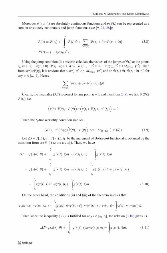
Moreover x(.), ex (.) are absolutely continuous functions and so Ψ(.) can be represented as asum an absolutely continuous and jump functions (see [9, 24, 28]):

Ψ 0ð Þ ¼ Ψ t0ð Þ þZt0

θ�Ψ tð Þdt þ

Xi∈N θð Þ

Ψ τ i þ 0ð Þ−Ψ τ i þ 0ð Þ½ � ;

N tð Þ ¼ i : τ i∈ t0; t½ �f g:

ð3:8Þ

Using the jump condition (iii), we can calculate the values of the jumps of Ψ(t) at the pointsτi, i=1, 2,…Ψ(τ i+0)−Ψ(τi −0)=< x(τi) −ex τ ið Þ , − xi

* > = −<x(τi), xi* >+MΦ τ ið Þ (xi*). Then

from x(τi)∈Φ(τi), it is obvious that <x(τi), xi* > ≤ MΦ τ ið Þ (xi*) and so Ψ(τi +0)−Ψ(τi −0) ≥ 0 for

any τi ∈ [t0, θ]. Hence Xi∈N θð Þ

Ψ τ i þ 0ð Þ−Ψ τ i−0ð Þ½ �≥0:

Clearly, the inequality (3.7) is correct for any point t1 = θ, and then from (3.8), we find Ψ (θ) ≥Ψ (t0), i.e.,

x θð Þ−ex θð Þ;−x� θð ÞD E

≥ x t0ð Þ−ex t0ð Þ;−x� t0ð ÞD E

¼ 0:

Then the t1-transversality condition implies

x θð Þ;−x� θð Þh i≥ ex θð Þ;−x� θð ÞD E

>> MQ∩Φ θð Þ −x� θð Þð Þ: ð3:9Þ

LetΔJ = J [x(.), θ]−J [ex (.), t1] be the increment of Bolza cost functional J, obtained by thetransition from arc ex (.) to the arc x(.). Then, we have

ΔJ ¼ φ x θð Þ; θð Þ þZt0

θ

g x tð Þ; tð Þdt−φ ~x t1ð Þ; t1ð Þ −Zt0

t1

g ~x tð Þ; tð Þdt

¼ φ x θð Þ; θð Þ þZt0

θ

g x tð Þ; tð Þdt−φ x t1ð Þ; t1ð Þ−Zt0

t1

g x tð Þ; tð Þdt þ φ x t1ð Þ; t1ð Þ

þZt0

t1

g x tð Þ; tð Þdt−φ ~x t1ð Þt1ð Þ−Zt0

t1

g ~x tð Þ; tð Þdt: ð3:10Þ

On the other hand, the conditions (ii) and (iii) of the theorem implies that

φ x t1ð Þ; t1ð Þ−φ ~x t1ð Þ; t1ð Þ þZt0

t1

g x tð Þ; tð Þ−g ~x tð Þ; tð Þ½ � ≥− x� t1ð Þ; x t1ð Þ−~x t1ð Þh i−Zt0

t1

x� tð Þ; x tð Þ−~x tð Þh idt:

Then since the inequality (3.7) is fulfilled for any t ∈ [t0, t1], the relation (3.10) gives us

ΔJ ≥φ x θð Þ; θð Þ þZt0

θ

g x tð Þ; tð Þdt−φ x t1ð Þt1ð Þ−Zt0

t1

g x tð Þ; tð Þdt: ð3:11Þ


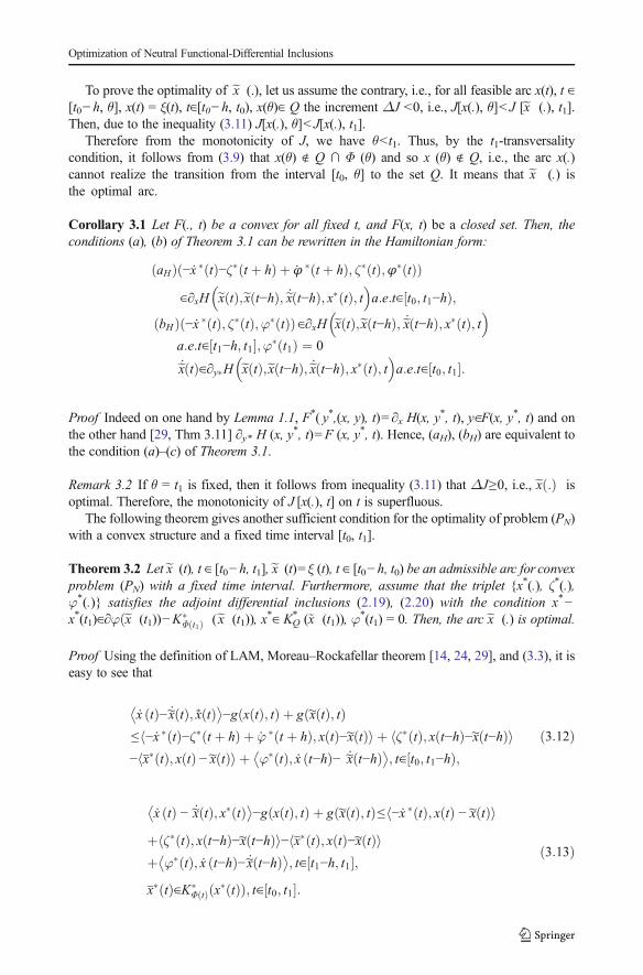
To prove the optimality of ex (.), let us assume the contrary, i.e., for all feasible arc x(t), t ∈[t0−h, θ], x(t) = ξ(t), t∈[t0−h, t0), x(θ)∈ Q the increment ΔJ <0, i.e., J[x(.), θ]<J [ex (.), t1].Then, due to the inequality (3.11) J[x(.), θ]<J[x(.), t1].

Therefore from the monotonicity of J, we have θ<t1. Thus, by the t1-transversalitycondition, it follows from (3.9) that x(θ) ∉ Q ∩ Φ (θ) and so x (θ) ∉ Q, i.e., the arc x(.)cannot realize the transition from the interval [t0, θ] to the set Q. It means that ex (.) isthe optimal arc.

Corollary 3.1 Let F(., t) be a convex for all fixed t, and F(x, t) be a closed set. Then, theconditions (a), (b) of Theorem 3.1 can be rewritten in the Hamiltonian form:

aHð Þ −x � tð Þ−ζ� t þ hð Þ þ φ � t þ hð Þ; ζ� tð Þ;φ� tð Þð Þ∈∂xH ex tð Þ;ex t−hð Þ; ex� t−hð Þ; x� tð Þ; t

� �a:e:t∈ t0; t1−h½ Þ;

bHð Þ −x � tð Þ; ζ� tð Þ;φ� tð Þð Þ∈∂xH ex tð Þ;ex t−hð Þ; ex� t−hð Þ; x� tð Þ; t� �

a:e:t∈ t1−h; t1½ �;φ� t1ð Þ ¼ 0ex� tð Þ∈∂y�H ex tð Þ;ex t−hð Þ;ex� t−hð Þ; x� tð Þ; t� �

a:e:t∈ t0; t1½ �:

Proof Indeed on one hand by Lemma 1.1, F*( y*,(x, y), t)=∂x H(x, y*, t), y∈F(x, y*, t) and onthe other hand [29, Thm 3.11] ∂y* H (x, y*, t)=F (x, y*, t). Hence, (aH), (bH) are equivalent tothe condition (a)–(c) of Theorem 3.1.

Remark 3.2 If θ = t1 is fixed, then it follows from inequality (3.11) that ΔJ≥0, i.e., ex :ð Þ isoptimal. Therefore, the monotonicity of J [x(.), t] on t is superfluous.

The following theorem gives another sufficient condition for the optimality of problem (PN)with a convex structure and a fixed time interval [t0, t1].

Theorem 3.2 Letex (t), t ∈ [t0−h, t1],ex (t)=ξ (t), t ∈ [t0−h, t0) be an admissible arc for convexproblem (PN) with a fixed time interval. Furthermore, assume that the triplet {x*(.), ζ*(.),φ*(.)} satisfies the adjoint differential inclusions (2.19), (2.20) with the condition x*−x*(t1)∈∂φðex (t1))−K�

Φ t1ð Þ (ex (t1)), x*∈ KQ

* (~x (t1)), φ*(t1) = 0. Then, the arc ex (.) is optimal.

Proof Using the definition of LAM, Moreau–Rockafellar theorem [14, 24, 29], and (3.3), it iseasy to see that

x tð Þ− �~x tð Þ; x� tð Þ� −g x tð Þ; tð Þ þ g ~x tð Þ; tð Þ

≤ −x � tð Þ−ζ� t þ hð Þ þ φ � t þ hð Þ; x tð Þ−~x tð Þh i þ ζ� tð Þ; x t−hð Þ−~x t−hð Þh i− x� tð Þ; x tð Þ −~x tð Þh i þ φ� tð Þ; x t−hð Þ− �~x t−hð Þ�

; t∈ t0; t1−h½ Þ;ð3:12Þ

x tð Þ − �~x tð Þ; x� tð Þ� −g x tð Þ; tð Þ þ g ~x tð Þ; tð Þ≤ −x � tð Þ; x tð Þ − ~x tð Þh i

þ ζ� tð Þ; x t−hð Þ−~x t−hð Þh i− x� tð Þ; x tð Þ−~x tð Þh iþ φ� tð Þ; x t−hð Þ− �~x t−hð Þ�

; t∈ t1−h; t1½ �;x� tð Þ∈K�

Φ tð Þ x� tð Þð Þ; t∈ t0; t1½ �:

ð3:13Þ


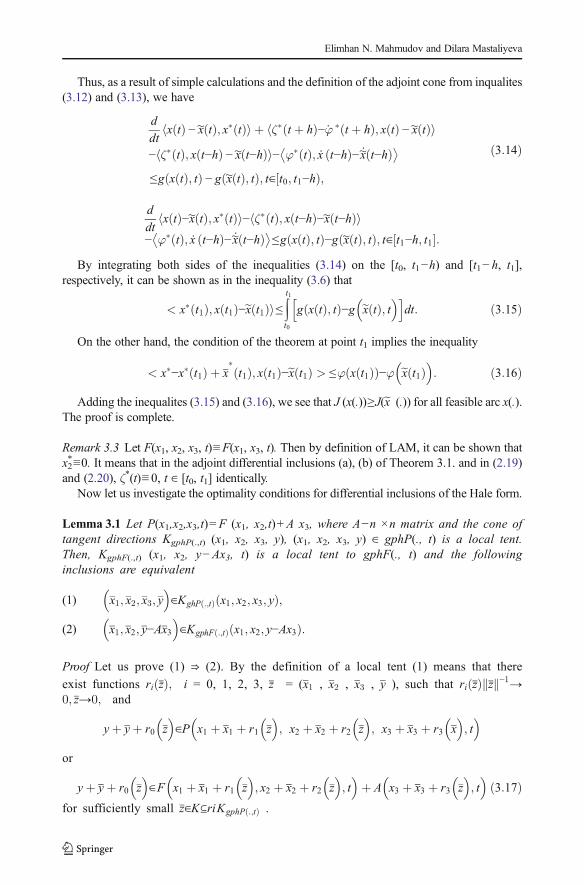
Thus, as a result of simple calculations and the definition of the adjoint cone from inqualites(3.12) and (3.13), we have

d

dtx tð Þ −~x tð Þ; x� tð Þh i þ ζ� t þ hð Þ−φ � t þ hð Þ; x tð Þ −~x tð Þh i

− ζ� tð Þ; x t−hð Þ −~x t−hð Þh i− φ� tð Þ; x t−hð Þ− �~x t−hð Þ� ≤g x tð Þ; tð Þ − g ~x tð Þ; tð Þ; t∈ t0; t1−h½ Þ;

ð3:14Þ

d

dtx tð Þ−~x tð Þ; x� tð Þh i− ζ� tð Þ; x t−hð Þ−~x t−hð Þh i

− φ� tð Þ; x t−hð Þ− �~x t−hð Þ� ≤g x tð Þ; tð Þ−g ~x tð Þ; tð Þ; t∈ t1−h; t1½ �:

ð3:13Þ

By integrating both sides of the inequalities (3.14) on the [t0, t1−h) and [t1−h, t1],respectively, it can be shown as in the inequality (3.6) that

< x� t1ð Þ; x t1ð Þ−ex t1ð Þi≤Zt1t0

g x tð Þ; tð Þ−g ex tð Þ; t� �h i

dt: ð3:15Þ

On the other hand, the condition of the theorem at point t1 implies the inequality

< x�−x� t1ð Þ þ x�t1ð Þ; x t1ð Þ−ex t1ð Þ > ≤φ x t1ð Þð Þ−φ ex t1ð Þ

� �: ð3:16Þ

Adding the inequalites (3.15) and (3.16), we see that J (x(.))≥J(ex (.)) for all feasible arc x(.).The proof is complete.

Remark 3.3 Let F(x1, x2, x3, t)≡F(x1, x3, t). Then by definition of LAM, it can be shown thatx2*≡0. It means that in the adjoint differential inclusions (a), (b) of Theorem 3.1. and in (2.19)and (2.20), ζ*(t)≡0, t ∈ [t0, t1] identically.

Now let us investigate the optimality conditions for differential inclusions of the Hale form.

Lemma 3.1 Let P(x1,x2,x3,t)=F (x1, x2,t)+A x3, where A−n ×n matrix and the cone oftangent directions KgphP(.,t) (x1, x2, x3, y), (x1, x2, x3, y) ∈ gphP(., t) is a local tent.Then, KgphF(.,t) (x1, x2, y−Ax3, t) is a local tent to gphF(., t) and the followinginclusions are equivalent

(1) x1; x2; x3; y� �

∈KghP :;tð Þ x1; x2; x3; yð Þ;

(2) x1; x2; y−Ax3� �

∈KgphF :;tð Þ x1; x2; y−Ax3ð Þ:

Proof Let us prove (1) ⇒ (2). By the definition of a local tent (1) means that there

exist functions ri zð Þ; i = 0, 1, 2, 3, z = (x1 , x2 , x3 , y ), such that ri zð Þ zk k−1→0; z→0; and

yþ yþ r0 z� �

∈Ρ x1 þ x1 þ r1 z� �

; x2 þ x2 þ r2 z� �

; x3 þ x3 þ r3 x� �

; t� �

or

yþ yþ r0 z� �

∈F x1 þ x1 þ r1 z� �

; x2 þ x2 þ r2 z� �

; t� �

þ A x3 þ x3 þ r3 z� �

; t� �

ð3:17Þfor sufficiently small z∈K⊆riKgphP :;tð Þ .


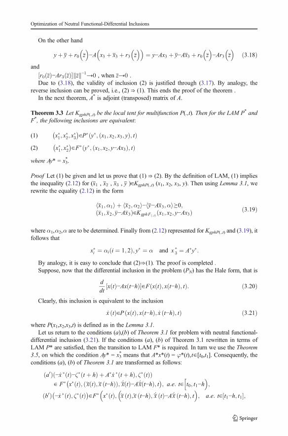
On the other hand

yþ yþ r0 z� �

−A x3 þ x3 þ r3 z� ��

¼ y−Ax3 þ y−Ax3 þ r0 z� �

−Ar3 z� �

ð3:18Þand

r0 zð Þ−Ar3 zð Þ½ � zk k−1→0 , when z→0 .Due to (3.18), the validity of inclusion (2) is justified through (3.17). By analogy, the

reverse inclusion can be proved, i.e., (2) ⇒ (1). This ends the proof of the theorem .In the next theorem, A* is adjoint (transposed) matrix of A.

Theorem 3.3 Let KgphP(.,t) be the local tent for multifunction P(.,t). Then for the LAM P* andF*, the following inclusions are equivalent:

(1) x�1; x�2; x

�3

� ∈P� y�; x1; x2; x3; yð Þ; tð Þ

(2) x�1; x�2

� ∈F� y�; x1; x2; y−Ax3ð Þ; tð Þ

where Ay* = x3*.

Proof Let (1) be given and let us prove that (1) ⇒ (2). By the definition of LAM, (1) impliesthe inequality (2.12) for (x1 , x2 , x3 , y )∈KgphP(.,t) (x1, x2, x3, y). Then using Lemma 3.1, werewrite the equality (2.12) in the form

x�1;α1h i þ x�2;α2h i− y�−Ax�3;αh i≥0;x�1; x

�2; y

�−Ax�3ð Þ∈KgphF :;tð Þ x1; x2; y−Ax3ð Þ ð3:19Þ

where α1,α2,α are to be determined. Finally from (2.12) represented for KgphP(.,t) and (3.19), itfollows that

x�i ¼ αi i ¼ 1; 2ð Þ; y� ¼ α and x �3 ¼ A�y�:

By analogy, it is easy to conclude that (2)⇒(1). The proof is completed .Suppose, now that the differential inclusion in the problem (PN) has the Hale form, that is

d

dtx tð Þ−Ax t−hð Þ½ �∈F x tð Þ; x t−hð Þ; tð Þ: ð3:20Þ

Clearly, this inclusion is equivalent to the inclusion

x tð Þ∈P x tð Þ; x t−hð Þ; x t−hð Þ; tð Þ ð3:21Þwhere P(x1,x2,x3,t) is defined as in the Lemma 3.1.

Let us return to the conditions (a),(b) of Theorem 3.1 for problem with neutral functional-differential inclusion (3.21). If the conditions (a), (b) of Theorem 3.1 rewritten in terms ofLAM P* are satisfied, then the transition to LAM F* is required. In turn we use the Theorem3.5, on which the condition Ay* = x3

* means that A*x*(t) = φ*(t),t∈[t0,t1]. Consequently, theconditions (a), (b) of Theorem 3.1 are transformed as follows:

a0ð Þ −x � tð Þ−ζ� t þ hð Þ þ A�x � t þ hð Þ; ζ� tð Þð Þ∈ F� x� tð Þ; ~x tð Þ;~x t−hð Þð Þ; �~x tð Þ−A �~x t−hð Þ; t�

; a:e: t∈ht0; t1−h

�;

b0ð Þ −x � tð Þ; ζ� tð Þ� ∈F� x� tð Þ;

�~x tð Þ;~x t−hð Þ; �~x tð Þ−A �~x t−hð Þ; t

� �; a:e: t∈ t1−h; t1½ �;


For the condition (c), we do the following notice. Let HF and HP be Hamiltonian functionsfor multifunctions F and P, respectively. It is easy to see that

HP x1; x2; x3; y�; tð Þ ¼ x3;A

�y�h i þ H F x1; x2; y�; tð Þ

and so argmaximum sets for multifunctions F and P are connected with equality

P x1; x2; x3; y�; tð Þ ¼ y∈P x1; x2; x3; tð Þ : y; y�h i ¼ HP x1; x2; x3; y

�; tð Þf g¼ y1∈F x1; x2; tð Þ : y1; y

�h i ¼ H F x1; x2; y�; tð Þf g ¼ F x1; x2; y

�; tð Þ; y1 ¼ y−Ax3:ð3:22Þ

Thus using the formula (3.22), we insure that the condition (c) of Theorem 3.1 is trans-formed as

c0ð Þ d

dtex tð Þ−Aex t−hð Þh i

∈F x tð Þ; x t−hð Þ; x� tð Þ; tð Þ; a:e: t∈ t0; t1½ �:

Note that (a ′)−(c ′) should be fulfilled for all x∈Φ(t).

Corollary 3.2 Letex :ð Þ be any feasible trajectory of the problem (PN) with differential inclusionof the Hale form (3.20) and let there exist a pair of feasible solutions {x*(.),ζ*(.)} of adjointinclusion, satisfying the conditions (a ′)−(c ′). Moreover, let the remaining conditions of Theo-rem 3.1 be fulfilled. Then ex :ð Þ is optimal.

4 Sufficient Condition for Optimality in Problem (PV)

Let us return to the problem (PV) and formulate the theorem for the sufficiency of arc ex (.).Moreover, let t = r(τ) be a solution of the equation τ = t−h(t) or the inverse function of τ.

Theorem 4.1 Assume ex (.) be some feasible solution of the problem (PV) and the pair offunctions {x*(.) ζ (.)}, satisfy almost everywhere the following conditions where ζ*(.) is anabsolutely continuous and x*(.) is a sum of absolutely continuous function and jump function:

(a) −x � tð Þ−r tð Þζ� r tð Þð Þ; ζ� tð Þð Þ∈F� x� tð Þ; ~x tð Þ; ~x t−h tð Þ; �~x tð Þ� ; t

� a:e:

t∈ t0; t1−h t1ð Þ½ Þ;

(b) −x � tð Þ; ζ� tð Þð Þ∈F� x� tð Þ; ~x tð Þ; ~x t−h tð Þð Þ; �~x tð Þ; t� a:e: t∈ t1−h t1ð Þ; t1½ �;

(c)�~x tð Þ∈F ex tð Þ;ex t−h hð Þð Þ; x� tð Þ; t

� �a:e: t∈ t0; t1½ �

which should be fulfilled for all x ∈ Φ (t). Then under the conditions (i)–(iv) of Theorem 3.1, thearc ex (.) is optimal in problem (PV).

Proof We remind that one of the distinctive places in the proof of Theorem 3.1 is the inequalities(3.4), (3.5). As is mentioned in the Remark 3.3 in the presented case, F(x1, x2, x3, t)≡F(x1, x2, t)


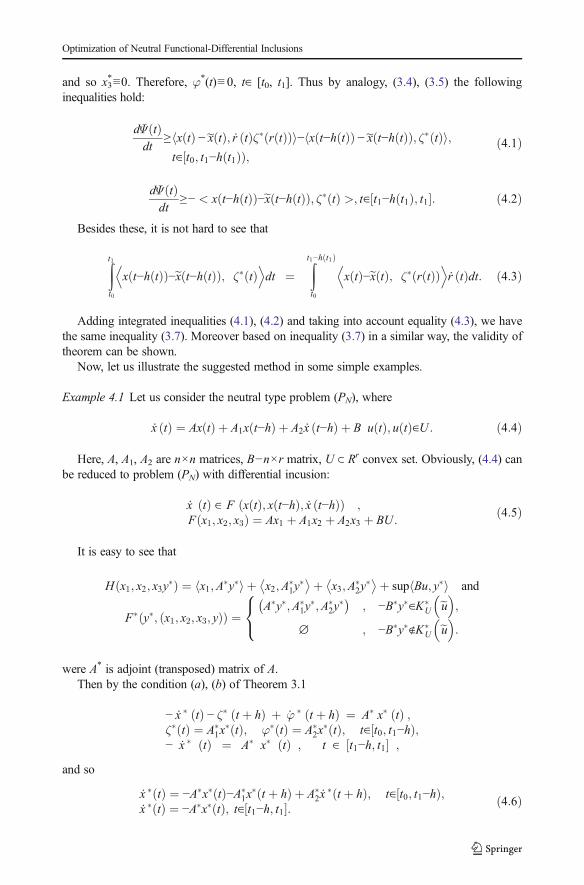
and so x3*≡0. Therefore, φ*(t)≡0, t∈ [t0, t1]. Thus by analogy, (3.4), (3.5) the following

inequalities hold:

dΨ tð Þdt

≥ x tð Þ −~x tð Þ; r tð Þζ� r tð Þð Þh i− x t−h tð Þð Þ −~x t−h tð Þð Þ; ζ� tð Þh i;t∈ t0; t1−h t1ð Þ½ Þ;

ð4:1Þ

dΨ tð Þdt

≥− < x t−h tð Þð Þ−ex t−h tð Þð Þ; ζ� tð Þ >; t∈ t1−h t1ð Þ; t1½ �: ð4:2Þ

Besides these, it is not hard to see that

Zt0

t1

x t−h tð Þð Þ−ex t−h tð Þð Þ; ζ� tð ÞD E

dt ¼Zt1−h t1ð Þ

t0

x tð Þ−ex tð Þ; ζ� r tð Þð ÞD E

r tð Þdt: ð4:3Þ

Adding integrated inequalities (4.1), (4.2) and taking into account equality (4.3), we havethe same inequality (3.7). Moreover based on inequality (3.7) in a similar way, the validity oftheorem can be shown.

Now, let us illustrate the suggested method in some simple examples.

Example 4.1 Let us consider the neutral type problem (PN), where

x tð Þ ¼ Ax tð Þ þ A1x t−hð Þ þ A2x t−hð Þ þ B u tð Þ; u tð Þ∈U : ð4:4Þ

Here, A, A1, A2 are n×n matrices, B−n×r matrix, U ⊂ Rr convex set. Obviously, (4.4) canbe reduced to problem (PN) with differential incusion:

x tð Þ ∈ F x tð Þ; x t−hð Þ; x t−hð Þð Þ ;F x1; x2; x3ð Þ ¼ Ax1 þ A1x2 þ A2x3 þ BU :

ð4:5Þ

It is easy to see that

H x1; x2; x3y�ð Þ ¼ x1;A

�y�h i þ x2;A�1y

�� þ x3;A�2y

�� þ sup Bu; y�h i and

F� y�; x1; x2; x3; yð Þð Þ ¼A�y�;A�

1y�;A�

2y��

; −B�y�∈K�U eu� �

;

∅ ; −B�y�∉K�U eu� �

:

8<:were A* is adjoint (transposed) matrix of A.

Then by the condition (a), (b) of Theorem 3.1

− x � tð Þ − ζ� t þ hð Þ þ φ � t þ hð Þ ¼ A� x� tð Þ ;ζ� tð Þ ¼ A�

1x� tð Þ; φ� tð Þ ¼ A�

2x� tð Þ; t∈ t0; t1−h½ Þ;

− x � tð Þ ¼ A� x� tð Þ ; t ∈ t1−h; t1½ � ;

and so

x � tð Þ ¼ −A�x� tð Þ−A�1x

� t þ hð Þ þ A�2x

� t þ hð Þ; t∈ t0; t1−h½ Þ;x � tð Þ ¼ −A�x� tð Þ; t∈ t1−h; t1½ �: ð4:6Þ


Besides, taking into account the conditions –B*y*∈KU* (eu ) and (c) of Theorem 3.1, we have

x� tð Þ;Beu tð ÞD E

¼ supu∈U

x� tð Þ;Buh i ð4:7Þ

where eu (.) is a controlling parameter corresponding to ex (.). Thus, the conditions (a), (b), (c)of the Theorem 3.1 for problem (PN) with (4.4), (4.5) consist of the conditions (4.6), (4.7). Letus rewrite (4.4) or (4.5) in the form:

d

dtx tð Þ−Ax t−hð Þ½ �∈F x tð Þ; x t−hð Þð Þ a:e: t∈ t0; t1½ � ð4:8Þ

where F1(x1,x2) = A x1+A1x2+BU. Let us write out the conditions (a ′)−(c ′) of Corollary 3.2.On the construction, it is perfectly clear that the problem (PN) with (4.5) and (4.8) has the samesufficient conditions. In fact, one can easily check

F�1 y�; x1; x2; y−A2x3ð Þð Þ ¼

A�y�;A�1y

�� ; if−B�y�∈K�

U eu� �;∅; if−B�y�∈K�

U eu� �:8<:

Then, the conditions (a ′)−(c ′) of Corollary 3.2 have the form:

x � tð Þ − ζ� t þ hð Þ þ A�x � t þ hð Þ ¼ A�0x

� tð Þ� ;

ζ� tð Þ ¼ A�1 x

� tð Þ a : e : t ∈ t0; t1−h½ Þ ;x � tð Þ ¼ −A�

0x� tð Þ; ζ� tð Þ ¼ A�

1x� tð Þ a:e: t∈ t1−h; t1½ �;

or

d

dtx� tð Þ−A�x� t þ hð Þ½ � ¼ −A�

0x� tð Þ−A�

1x� t þ hð Þ a:e: t∈ t0; t1−h½ Þ;

x � tð Þ ¼ −A�0 x

� tð Þa :e : t∈ t1−h; t1½ �ð4:9Þ

and in the presented case the condition (c ′) simply consists of (4.7).

Example 4.2 Now let us consider the problem (PV) with the differential equation and variabledelay:

x tð Þ ¼ Ax tð Þ þ A1x t−h tð Þð Þ þ Bu tð Þ; u tð Þ∈V : ð4:10ÞA, A1 are n×n matrices, B−n×r matrix, V⊂Rr– is convex set. Let us replace (4.10) with the

differential inclusion:

x tð Þ ∈ F x tð Þ; x tð Þ; x t−h hð Þð ÞðF x1; x2ð Þ ¼ Ax1 þ A1x2 þ BV :

ð4:11Þ

Demonstrating the similar calculation of Example 4.1, we can conclude that the conditions(a),(b) of Theorem 4.1 can be converted to

−x � tð Þ−ζ� r tð Þð ÞÞ x tð Þ ¼ A�x� tð Þ; t∈ t0; t1−h t1ð Þ½ Þ;ζ� tð Þ ¼ A�

1 x� tð Þ ;

−x � tð Þ ¼ A�x� tð Þ; t∈ t1−h t1ð Þ; t1½ �;ð4:12Þ

respectively.


Finally, (4.12) can be rewritten as follows:

x � tð Þ ¼ −A�x� tð Þ−A�1x

� r tð Þð Þr tð Þ; t∈ t0; t1−h t1ð Þ½ �; ð4:13Þ

x � tð Þ ¼ −A�x� tð Þ; t∈ t1−h t1ð Þ; t1½ �: ð4:14ÞThat is the conditions (a), (b), (c) of the Theorem 4.1. for stated problem consist of the

conditions (4.13), (4.14), and (4.7), respectively. Thus, the examples 4.1 and 4.2 show that forthe concrete problems the conditions of the proved theorems and well known results ofclassical optimal control theory coincides. In this way, the reader can consult for more detailedinformation of Mordukhovich [24] and Gabasov and Kirillova [9].

References

1. Agrachev AA, Sachkov YL. Control theory from the geometric viewpoint, control theory and optimizationII. Berlin: Springer; 2004.

2. Aubin JR, Cellina H. Differential inclusion, Springer,Grudlehnender Mat., Wiss.,1984.3. Viorel Barbu. Convexity and optimization in Banach Spasces, Sijthoff (1978). 2nd ed. Dordrecht:

D.Reiderel; 1986.4. Barbu V. Analysis and control of infinite dimensional systems. New York: Academic; 1983.5. Clarke FH. Optimization and nonsmooth analysis. New York: Wiley-Interscience; 1983.6. Clarke FH, Wolenski PR. Necessary conditions for functional differential inclusions. Appl Math Optim.

1996;34:34–51.7. Clarke FH. Hamiltonian analysis of the generalized problem of Bolza. Trans AmMath Soc. 1987;301:385–400.8. Demyanov VF, Vasilev LV. Nondifferentiable optimization. New York: Optimization Software; 1985.9. Gabasov R, Kirillova FM. Maximum principle in theory of optimal control. Minsk: Nauka i Teknika; 1974.10. Hale J. Theory of functional differential equations. New York: Springer; 1977.11. Haddad G. Topological properties of the sets of solutions for functional differential inclusions, Nonlinear

Analysis, 2001;5(12):1349–1366.12. Haddad G, Lasry JM. Periodic solutions of functional differential inclusions and fixed points of σ-

selectionable correspondences. J Math Anal Appl. 1983;96(2):295–312.13. Hernandez E, Henriquez HR. Existence results for partial neutral functional differential equations with

unbounded delay. J Math Anal Appl. 1998;221:452–75.14. Ioffe AD, Tikhomirov VM. Theory of extremal problems, Nauka, Moscow, 1974 (in Russian); English

transl., North-Holland, Amsterdam; 1979.15. Loewen PD, Rockafellar RT. The adjoint arc in nonsmooth optimization. Trans AmMath Soc. 1991;325:39–72.16. Kolmanovskii VP, Shaikhet LE. Control of systems with aftereffect. New York: Academic; 1996.17. Mahmudov EN. Approximation and optimization of discrete and differential inclusions. Waltham, MA:

Elsevier; 201118. Mahmudov EN. Optimal control of cauchy problem for first-order discrete and partial differential inclusions.

J Dyn Control Syst. 2009;15(4):587–610.19. Mahmudov EN. Locally adjoint mappings and optimization of the first boundary value problem for

hyperbolic type discrete and differential inclusions. Nonlinear Anal, 2007;67(10):2966–2981.20. Mahmudov EN. Sufficient conditions for optimality for differential inclusions of parabolic type and duality. J

Glob Optim. 2008;41(1):31–42.21. Mahmudov EN. On duality in problems of optimal control described by convex differential inclusions of

Goursat-Darboux type. J Math Anal Appl. 2005;307:628–40.22. Mahmudov EN. The optimality principle for discrete and first order partial differential inclusions. J Math

Anal Appl. 2005;308:605–19.23. Mahmudov EN. Optimization of differential inclusions of Bolza type with state constraints and Duality.

Math J. 2005;7(N2):21–38.24. Mordukhovich BS. Variational analysis and generalised differentiation I, II, Grundlehren der mathematischen

Wissenschaften. 2006 Vol. 330,331.25. Mordukhovich BS, Wang L. Optimal control of neutral functional-differential inclusions linear in velocities.

TEMATend Mat Apl Comput. 2004;5(1):1–15.


26. Medhin NG. On optimal control of functional-differential systems. J Optim Theory Appl. 1995;85:363–76.27. Outrata J, Mordukhovich BS. Coderivative analysis of quasivariational inequalities with applications to

stability and optimization. SIAM J Optim. 2007;18:389–412.28. Pontryagin LS, Boltyanskii VG, Gamkrelidze RV,Mishchenko EF. The mathematical theory of optimal

processes. New York: Wiley; 1965.29. Pshenichnyi BN. Convex analysis and extremal problems. Moscow: Nauka; 1980 (Russian).30. Rowland JDL, Vinter RB. Dynamic optimization problems with free time and active state constraints. SIAM

J Control Optim. 1993;31:677–91.31. Rubinov AM. Superlinear multivalued mappings and their applications to economical–mathematical prob-

lems. Leningrad: Nauka; 1980 (in Russian).32. Richard L, Yung CH. Optimality conditions and duality for a non-linear time delay control problem. Optim

Control Appl Methods. 1997;18(5):327–40.33. Hong S. Boundary-value problems for first and second order functional differential inclusions. Electron J

Differ Equ. 2003;32:1–10.34. Vinter R, Zheng HH. Necessary conditions for free end-time measurably time dependent optimal control

problems with state constraints. Set-Valued Anal. 2000;8:11–29.35. Zhu QJ. Necessary optimality conditions for nonconvex differential inclusion with endpoint constraints. J

Diff Equat. 1996;124:186–204.


optimization of neutral functional-differential inclusions

Documents