optimization in thin-layer chromatography : some practical considerations

CHROM. 13.600

OPTIMIZATION IN THIN-LAYER CHROIMATOGRAPHY

SOME PRACTICAL CONSIDERATIONS*

The application of the results of ;I prex iqus optimization theor> of thin-l,i>cr clironiatograpl~~ is discussed 11 ith rel‘erencc to problems of‘ current Interest to ana- l>t~cul chemists. Experimental cl ldcnce of’ the \alidit> and of‘ the practical interest of the equations deri\ ed is gi\ en. Pro\ ided the retention factors. R, _ of ;I series of‘ compounds and the plate number necessary to achieve the requested degree of resolution bet\\een the spots of these compounds are kno\\n. it is as> to c:ilcul,itt‘ the p,tr-tick size and development length ~~hich 1 ield the minimum an:tl>sis time.

Examples taken tiotn either the literature or experiments descrtbed here dem- onstrate that. \\hile easy separations can be performed on plates with small partick stzes in a short limp _ and x\ith a \eq small dtxelopment lengh. dtliicult scpar,ttions need coarser particles. greater de\ elopment lengths and are slo\x er. The most tmpor- tant parameter xx hich determines the minimum artal>sis time is the ditt‘usion cwlficicnt of‘ the solute’. and the diw-cpancirs that map OCCLII- bet~ctm obscrxed and predicted analysis times most olicn ,irisc from the error in the c’sl~~n,illciri of the dilt‘usion C0dfCllX11S.

130 A. M. SIOUFFI, F. BRESSOLLE, G. GUIOCHON

rations obtained on such packings led to the needless acronym HPTLC (high-performance thin-layer chromatography). In practice, an analyst carrying out TLC is attract-

ed by the simplicity and the efficiency of the method; he is not necessarily interested in its ultimate performance but in the resohttion of his own separation problems.

As early as 1976, it was demonstrated’ that TLC plates prepared with very fine particles (5 pm) did not in many cases give better performance than regular plates. Since then the advent of nanoplates has given rise to further controversy’. In an effort to elucidate the origin of this problem we reconsidered the parameters involved in TLC. In previous papers 36 theoretical equations were developed to relate development time, efficiency and resolution to the parameters describing the plate, the chromatographic system and the separation, and a general scheme of optimization was set

up. The aim of the present work is to provide experimental evidence of the validity

of these equations and to supply the analyst with the theoretical background to what is possible in TLC and what is not. A few guidelines will permit an estimate of the cost of a given analysis provided some initial conditions such as the plate number and the retention are known.

EXPERIMENTAL

Two types of plates were used: commercially available TLC and HPTLC plates from E. Merck (Darmstadt, G.F.R.) and home-made plates. The latter were obtained by spreading a silica slurry in carbon tetrachloride on a glass plate, followed by evaporation of the solvent and activation for 1 h at 110°C. In both cases the layer thickness is 0.25 mm.

Merck plates are made with 1 l-15 pm particles (TLC plates) and 5-7 pm particles (HPTLC plates), and have a rather narrow particle size distribution. We used LiChrosorb Si 60 having similar particle sizes and particles prepared from a batch of silica supplied by I. Hal&z (Saarbrtlcken, G-F-R.). A Bacco classifier permitted the preparation of a 243 l-pm particle sample.

LiChrosolv-type solvents were used without further purification. Sample de- position was performed with glass capillaries of internal diameter 0.1 mm. One drop of solution was spotted to prevent circular spreading of the solute on the plate. Conventional developments were carried out in a Camag chamber with a ground glass lid. Densitograms were recorded with a Zeiss PMQ II spectrophotodensitometer at a plate speed of 20 mm/min.

THEORETICAL

The following equations were derived in previous papers3*, to which the reader is referred for a discussion of the ranges of validity.

The b&c eqrratiom As the capillary rise occurs in the plates the distance, I, between the solvent

front and the solvent source is related to time, t, by

2 - =kt (1)

OPTIMIZATION IN TLC 131

with

(2)

where k is the velocity constant of the solvent, cI, the particle diameter, 7 the solvent surface tension and rl its viscosity; k, is a dimensionless coefficient, close to S - 10e3 (ref. 4). The influence of the wetting angle of the solvent on the adsorbent has been neglected in eqn. 2. This effect can be important in reversed-phase TLC.

At the end of the development, the migration distance of the solvent is L, the migration distance of the spot is X and by definition of the retention factor, R,:

X = R,L (3)

The plate number isgiven by:

x2 N=16 F 0 (4)

IV is the spot width which can be measured with accuracy only on a densitogram’. The resolution between two spots 1 and 2 of Gaussian profile is:

By analogy with the conventional definition of the plate height. Snyder” has shown that

LRF N = - H

(6)

where His the average height equivalent to a theoretical plate; His a function of the development length, the retention factor and the diffusion coefficient. The plate number necessary to achieve the resolution, R, between two solutes of relative retention

where X-f is the bed capacity factor for compound i

l - RF.i /if= R_

F.1

is given by:

(1 + k’)’ k”

(7)

(8)

(9)


Let us assume that the local plate height is given by the conventional reduced plate height (It) equation used in column chromatography9

1~ = !! + As"3 + Cv (10) 1'

wnh

(11)

where II is the flow-velocity, A characterizes the quality of the packing, C the resist- ance to mass transfer in the chromatographic bed and B the axial diffusion in that bed. Previous_calculations and experiments have shown that A is approximately unity for most correctly prepared plate$, that C is usually small (0.01-0.03) and that B is given by

(12)

where D, is the diffusion coefficient in the mobile phase, yrn the tortuosity coefficient of the bed and D, and yS the corresponding terms for the stationary phase. Two cases are possile depending on whether -y,D, is negligible or comparable in magnitude to

3’Z-n In- D It is easy to show5 that the average plate height is given by:

where z. is the distance of the sample spot above the solvent level in the tank. Be- cause C is small, in practice the third term of eqn. 13 is negligible. Fig. 1 shows plots of average plate height IWXIS development length calculated for various particle sizes. These plots show the dramatic influence of the diffusion coefficient with fine particle? since for dp c 10 pm we can write

B H = oc!,‘(i + zo)

and B is proportional to the diffusion coefficient_ The influence of D, is less dramatic with coarse particies since for larger particle sizes we can write

(14b) H = b(L + zo) + a- L2/3

L I_“” -0

B 3 Aa”pl’ 01’3 withb=- and a=-.

OdP 2 (2 0,)“”


I . L b-4 , 0 5 lo 15 xl

Fig. 1. Plots of the average height equivalent to a theoretical plate, If, wrsus developmktt length, L, for various particle sizes. A = 1; 7 = 0.70; D, = 5. IOm6 cm’/sec; C = 0.01; RF = 0.70; ymD, = y,D,; 0 = 70 cm/set; z0 = 0.5 cm. The number on each curve is the particle size.

and the coefficient (z is proportional to 0; 1’3 For particle sizes between 10 and 20 pm . the two terms are comparable and their variations compensate each other so H is almost constant.

Tile principles of optimization From the plots of Fig. 1 it is evident that the efficiency of coarse particle plates

improves with increasing development length, while the opposite is true for fine particles. Usually development is carried out for 10 cm since the calculation of R, is made easier and efficiency is good enough. In some cases it is worth using longer distances_ This was demonstrated experimentally by Vemin” who separated essential oils with a development length of 15 cm using plates with 40-pm particles. It must be emphasized that development on 10 cm is not the rule and that different distances may be more appropriate. The analysis time may vary widely with the particle size used’.‘.

To carry out a given separation a number of theoretical plates, IV,,, given by eqn. 9 is needed. According to eqn. 6 we can write:

RF H _=- Nne L

(1%

The development length and the particle size are thus determined by the intersection with the N = f(L) curves in Fig. 1 of the straight line of slope &IN,,, passing through the origin. There are as many solutions as we have batches of the selected stationary


phase of different particle size. The best combination is that which gives the shortest analysis time or, as shown by eqns. 1 and 3, the lowest value of L2/dp6.

For each problem the analyst may draw H versus L plots but this is time- consuming and until the calculation is finished he has no idea of the optimal conditions. Although these plots are quite informative, providing useful insight into the mode of TLC separations and the selection of good compromises, a more direct approach may be preferred especially in difficult cases. This is the direct calculation of the optimum conditions, using the equations derived previously6. The maximum mmber of plates which can be obtained in TLC is given by:

NM = ed&Jzf

2 i - &)I (16)

The of N,, not the for all on the plate but upon the of the system and the solute It takes infinite

amount time to N,, plates. the experimenta should be that N,, N,, and N,,, z

The minimum analysis time, E,.,, is given by

32

fR.rn =

16 D, lv3 0’ (17)

if we assume that -q ,,D,,, and ;‘,D, in eqn. 16 are equivalent. The corresponding optimum particle size is

4.0 = & I;I,D,& + (1 - RF) y,D,] N (1Sa) F

or, if we assume as before that ymD, = ;‘,D,:

Tne plate number, N, in eqns. 17 and 18 is that necessary for the given separation. The development length is given by:

(19)

In eqns. 17-19 it has been assumed that diffusion takes place in both stationary and mobile phases at the same rate so 7, D, = ;‘,D,. This is not always the case but it is the most unfavourable case, giving the largest values of cl,., (Fig. 3). of development length and analysis time6. If calculations are performed using these equations, the resolution obtained cannot be worse than predicted. The drawback of this type of approach is that it yields a particle diameter which is not available or a development length which is impractical. When optimum particle diameter is not available, it has


0 N

Fig. 3. Variation of the optimum particle diameter. d,,.,, with the number of plates, IV (cf-, eqn. ISa). Influence of the diffusion in the stationary phase. 7 = 0.75; D,,, = 5. 10m6 cm’iscc; 0 = 90 cm/set; R, = 0.5. Curves: 1 , ymDm = y,D,; 2, TED, = 0 or ;.,,,Dm = ysDs with D, = 2.5. 10e6 cm’jsec; 3,7,,,D, = ;‘_D,. D, = l_ 10es cm’jsec.

been shown that the analysis time does not increase greatly when the particles used are not more than 30 oA smaller or 50% larger than optimum6. If development length is impractical, it means either that the separation is impossible (L, too long) or very easy (L, too short) which should be obvious from the beginning. Thus the calculations

of &I and tR.m P ermit a rapid selection of the optimum experimental conditions.

These factors are obvious from the equation for H (eqns. 13 and 14a). As C is often small and the third term of eqn. 13 negligible compared to the first two.the main parameters are R,, A, D, and 0. Their influence has been discussed previously6.

As His a function of R,, d,_, and L, depend on the retention. It is important to select a chromatographic system which gives a value of R, somewhat larger than 0.33 but not much larger than 0.606.

A decrease of the packing term A results in a decrease in the analysis time and the development length. At present, it is easy to buy or prepare plates haking a packing term of unity. From our experience the influence of the binder on commercially available plates is rather small. A 10 oA decrease in A would result in a 15 % reduction of the analysis time (~5, eqn. 17). We made no attempt to improve the quality of the packing, however, as we think that the loss of efficiency due to the recording systems is more important”.

The diffusion coefficient, D,, is by far the most importardt factor when healing with small particles_ As soon as the mobile phase velocity has decreased below the optimum velocity which arrives for a development length which decreases rapidly with decreasing particle size6, the molecular diffusion controls the spot broadening. This is why spots in HPTLC are circular, diffusion taking place at comparable speed in the


stationary and mobile phases so that almost all spots (except for RF z 0) have the same diameter3. An increase in D, will result in a larger value of H and the separation of closely related compounds will be more difficult_ As illustrated in Figs. 2 and 3, it is much more difficult to generate large plate numbers when D, is of the order of 1 . 10m5 cm2/sec than when it is 5 - lob6 cm2/sec_ This explains why demonstrations performed with heavy lipophilic dyestuffs yield such beautiful spots and dramatic chromatograms.

Fig. 3. Variation of the optimal development length with the necessary plate number and the diffusion coefficient (cJ, eqn. 19). The number on each curve is equal to 10’. D, (cm’/sec). A = 1; y = 0.75; RF = 0.4; e = 70 cm/se%.

Because of the scarcity of experimental data, the diffusion coefficient, D,, is usually calculated through the Wilke-Chang equation12

D = 7.4. lo-’ (0 A+!’ T m

rl ( w”-6 (20)

where A4 is the molecular weight of the solvent, 0 its association constant, II its viscosity and V, the molar volume of the solute. Calculation of 0, first requires the

calculation of V, and an estimate of aI. When the density of the solute is unknown, the Le Bas method” is used to calculate VI\; however, this is not precise and a 10 y/, systematic error may occur between the actual and calculated V,. The association constant, 0, is estimated to be 1.0 for non-associated solvents such as hexane, chloroform or acetonitrile, and 2.6 for water. Great difficulties arise when a mixture of solvents is used; the calculation of D, becomes tedious, time-consuming and inac- curate. There is a severe lack of experimental data despite the promising determi- nation method published by Grushka and Kikta 13_ Unfortunately, these authors


studied diffusion of phenones in hexane, a solvent which does not move these solutes on silica gel plates, so we could not use their data.

As shown by eqns. 9 and 17, respectively, the efficiency increases and the analysis time decreases when D, decreases_ Nanoplates coated with small particles are suitable for the separation of low 0, solutes, as exemplified by the analysis of

phospholipids’” and the separation of digitoxin and digoxint5. Finally, more attention in the selection of the solvent should be paid to its

dynamic properties. Admittedly it is already difficult to select a development liquid while keeping the critical solute RF between 0.35 and 0.60. Eqn. 1 Sa, however, as well as plots of $, versm N as shown in Fig. 4, show that for constant eluotropic strength the larger 8 is the larger the plate number is which can be achieved using particles of a

given size. Thus hexane is a better solvent than octane and toluene better than benzene. Tables of velocity coefficients are available in the literature*.

I 0 SC0 Km N

Fig. 4. Variation of the optimum particle diameter with the necessary plate number. Influence of the velocity coelikient. The number on each curke is the value of 0 (eqn. 2). ymD, = y,D,; y = 0.75; R, = 0.4; 0, = 1 . IO-’ cm’pec. The hatched area corresponds to commercially available HPTLC plates (5 pm) or TLC plates (11 .um).

RESULTS AND DISCUSSION

Validity of the approach Before we discuss the optimization problem, we must emphasize that the chro-

matographic contribution to H only is involved in the curves in Fig. 1. In TLC as in other chromatographic processes the variance of the solute distribution is given by:

(21)

The extra column effects include those of injection and detection.

13s A. M. SIOUFFI, F. BRESSOLLE, G. GUIOCHON

Excehent sample spotting is required to keep the injection elect as smal1 as possible. Halpaap and Ripphahn16 have shown that it may be as large as 20 y0 of the total zone variance. Sample spotting using a microsyringe or glass capillaries is suitable if a very small amount of solution is delivered. Fi g. 5 shows recordings of injection spots which indicate the non-Gaussian shape of the sample band. When small samples are used profiles like that in Fig. 5a make only a small contribution to the band width because they are very steep. With a width of 1.5 mm these profiles have a variance contribution of 0.20 mm2 (ref. 1 l), CCL. 5 o/o of the chromatographic variance of a spot when L = 10cmand R, = 0.7 (cf-, Fig. 1). With larger samples we obtain profiles like that in Fig. 5b with a standard deviation of 0.8 mm and a contribution of ca. 20 %_ To overcome this difficulty plates with a concentration zone are now available”.

- 0 2 4 6 - F-

= b-4 Fig. 5. Recording of sample spots in reflection mode. a, Solute pyrene, detection by fluorescence. i.,,_ 280 XUTJ. I,,_ 375 MI, plate travel 0.5 mm/min. recorder chart speed 5 mm/min. b and c. Solute bis(chlorophenyl)triazene, UV detection, L 366 nm, plate travel 0.5 mm/min, recorder chart speed 10 mm/min. 2 = Actual distance on the TLC plate. b. Microsyringe; c. micropipette.

Provided a good spectrophotodensitometer is used the detector variance contribution is not too large, but with many instruments currently available it may still represent a very important contribution. It will be discussed in a forthcoming paper’ l.

The comparison between theoretical curves and experimental data made by Halpaap and Krebs I7 is very interesting. As seen in Fig. 6, there is a striking agreement which can be accounted for by assuming negligible extra-bed contributions. No information was given about the particle size, but Merck TLC plates are made with 1 l-15 pm particles and HPTLC plates with 5-7 pm particles4. The chemical formula of the lipophilic dyestuff used was also not given, but it is obviously a high-molecular- weight molecule and D, should lie between 5 - 10e6 and 10 - 10V6 cm’/sec. A long

OPTIlMIZATION IN TLC 139

a.

A I

D_

0 I

5 70 -

L km1

Fig. 6. Plots of H wrsrts L for data from ref. 17 (Table XIII). Dyestuffs: 0, >ioIet (D, = 6. IOe6 cm’kc. R, = 0.75, C = 0.10); 0, green (D, = 6- IO-” cm’/sec, R, = 0.45, C = 0.20); A. blue (D, = 4. 1O-6 cm’/sec, R, = 0.17, C = 0.20). Esperimental points and curves calculated with 0 = 70 cm/xc. 7 = 0.75, rl = 0.80 and d, = 15 pm for TLC plates (a); rl = 1.0 and dp = 7 pm for HPTLC plates (b). Curves: 1, blue: 1. green; 3, violet. The lower curves in b correspond to the assumption that 7,D, = 0.5 T&,,. All others to 7.Q = y,D,.

_ deveIopment was not performed on the HPTLC plate as HaIpaa~‘~*” \vas \vefl a\vare that small particles yield good efficiency only for short development distances.

A glance at the published chromatograms’6.” shows that some separations are best performed on TLC plates rather than on HPTLC ones. The explanation is provided by the theoretica curves of Fig. I. Easy separations can be performed with small particles over very short distances; difficult separations must be performed with coarser particles and longer development.

Examples of’application Consider first an easy separation: pyrene from chrysene. According to pre-

viously published data”, the capacity factors with the system n-hesane and silica are respectively 4.11 and 6.61. Calculation of the plate number necessary to achieve the separation yields 150 plates for a resolution of unity or 230 plates for R = 1.25 (c/I. eqn. 9). A very short development on a plate coated with small particles will be convenient. This is demonstrated in Fi,. 0 7 which shows densitograms obtained after 2 cm development on plates coated with particles of different size. The resolution obtained with 5-jlrn particles allows quantitation of very small amounts of one solute in


Fig. 7. Separation of pyrene and chrysene. Development length: 2 cm. Detection: fluorescence, L,,. 254 nm, A,. > 375 nm. a and b, Nanoplate silica (5 m). resolution 1.2; c, silica (1 I pm), resolution 0.75; d, silica (“0 pm), resolution 0.55. Developing solvent: hexane.

a mixture of both. It becomes poorer as the particle size increases while the development length is kept at 2 cm; at the same time the development time decreases like 7,2 and I.

Consider now the more difficult separation of bis(chlorophenyl)triazeneslg. The retention factors are given in Table I. In order to separate the isomers III-V we need about 1000 plates for R = 1, 1500 plates for R = 1.25. Since the separation was performed with carbon tetrachloride, 8 = 465. The calculation of the diffusion coef- ficienl using the Wilke and Chang formula” gives D, = 9 - lo-” cm”/sec, with an error of probably less than 10 ‘A_ Assuming y,D, = y,D, we can draw curves similar to those in Fig. 1, using the exact values of the parameters pertaining to the problem.

TABLE I TRIAZENES STUDIED

A-0. Conlpound Structure RF k

I II III IV v

Bis(3,5-dichlorophenyl)triazene Bis(&klichlorophenyl)triazene Bis(2,3,Ctrichlorophenyl)triazene Bis(2.3,5-trichlorophenyl)triazene

H H 0.10 H H H 2.6

H H 0.58 Cl Cl H 0.49

Cl Cl 0.78


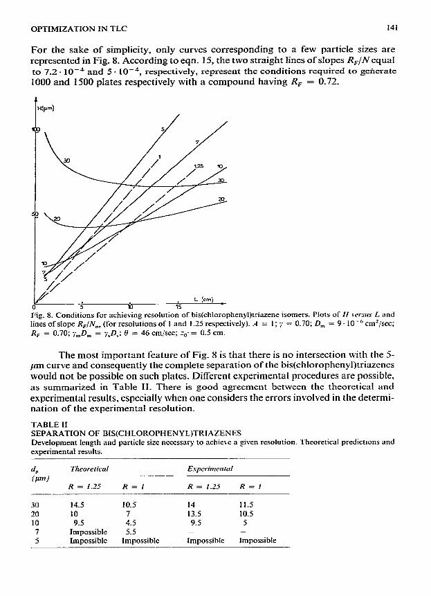
For the sake of simplicity, only curves corresponding to a few particle sizes are represented in Fig. 8. According to eqn. 15, the two straight lines of slopes R,/N equal to 7.2-1O-L and 5- 10e4, respectively, represent the conditions required to geherate 1000 and 1500 plates respectively with a compound having R, = 0.72.

t H!&

Fig. 8. Conditions for achieving resolution of bis(chlorophenyl)triazene isomers. Plots of If te~.w~ L and lines of slope RJIV_ (for resolutions of 1 and 1.25 respectively). A = I; ; = 0.70; D, = 9. 10e6 cm’/sec; RF = 0.70; i’, D, = i;D,; 0 = 46 cm/xc; zo- = 0.5 cm.

The most important feature of Fig. 8 is that there is no intersection with the 5- irrn curve and consequently the complete separation of the bis(chlorophenyl)triazenes would not be possible on such plates. Different experimental procedures are possible, as summarized in Table II. There is good agreement between the theoretical and experimental results, especially when one considers the errors involved in the determi- nation of the experimental resolution_

TABLE II SEPARATION OF BIS(CHLOROPHENYL)TRIAZENES Development length and particle size necessary to achieve a given resolution. Theoretical predictlons and experimental results.

4 Theorerical Esperimcnrul

(We) R = I.25 R=I R = 1.2-i R=l

30 20 10

7

5

14.5 10.5 14 11.5 10 7 13.5 10.5 9.5 4.5 9.5 5

Impossible 5.5 _ -

Impossible Impossible Impossible Impossible

A. M. SIOUFFI, F. BRESSOLLE, G. GUIOCHON

I I

E a

::

r


As shown by Fig. 1 and evidenced by Table III, with coarse particles H remains nearly constant for development lengths between 8 and 25 cm and consequently the efficiency increases in proportion to the development length. The results obtained with very small particles are slightly better than predicted, possibly because it is easier to prepare “good” plates, with A = 1, from small particles than from coarse ones. An- other reason is that the spectrophotodensitometer gives a lower contribution to the spot width when the development is long. It is obvious that the complete resolution of the mixture is impossible with very small particles.

TABLE III SEPARATION OF BIS(CHLOROPHENYL)TRIAZENES

Experimental data on plates of silica Si 60 having different particle sizes.

Particle size Dereeloprnent length Resolution

(PJl~) (nulI) III/IV IV/V

25-31 90 0.64 0.73 110 0.85 0.87 120 1.03 I.04 130 1.13 1.2’

‘0 105 0.89 1.01 130 1.06 1.27

11 55 0.93 1.08 95 1.13 1.25

5 35 0.78 0.70 40 0.88 0.85 50 0.86 0.90 SO 0.88 0.95

It must be emphasized also that the width of the particle size distribution is very important. This is illustrated in Fig. 9 which shows the same separation achieved using two different batches of 1 l-pm silica particles. When the size distribution is large or when a small amount of particles of different diameter is present the separation ability of the plate is dramatically reduced.

We consider now two other examples taken from the literature. Bidlo-Igloy” carried out the separation of the three monochloroaniline isomers in a U-chamber, after a Z-cm development w&h toluene (0 = 77) as solvent. Linear R, values calculated from the circular ones published are: Zchloroaniline, R, = 0.41, k’ = 1.44; 3- chloroaniline, R, = 0.24, k’ = 3.1. From separate calculations as explained above, we obtain 0, = I.9 - lo-’ cm’,kec and N,, = 100 (R = 1). A plot of H = f(L) (cj:. Fig. 10) shows that the separation is very easy using particles of small size and with a short development length, in agreement with published data. The predicted development length is 1.5 cm with 5-pm particles for R = 1. It would be about the same with IO-pm particles, however, and ca. 5 cm with 1%pm particles.

The last example is an analysis of aflatoxins ‘l The separation is difficult and . not complete during the first run. Aflatoxins are high-molecular-weight molecules (C17H1207 and Ci,H,,06) and D, = 5 - 10e6 cm2/sec in the developing solvent chloroform-acetone (90:10). If we assume that RF = 0.5, the N = f(L) plots show that, as for the separation of bis(chlorophenyl)triazenes, the aflatoxin separation is


Fip. 10. Plots of H wrm L used lo seiect the optimum conditions for the separation of chloroaniline isomers according to ref. 20. ysD, z 0; D, = 1.9.10-5 cm’/sec; A = 1; C = 0.01; y = 0.75; 0 = 77 cmkec.

impossible on 5-pm particle plates since the RF/Nn, line does not intercept the 5-pm or 7-jtm curve. This result illustrates the fact discussed above, that there is a limit to the number of plates that one can expect from a thin-layer chromatographic plate (cj:, eqn. 16). In this case again IO- or 20-pm particles would give the best results.

Practice of optirkatioi2 In practice, optimization is possible only if the analytical aim can be stated

precisely, which means that some characteristics of the separation must be known. For unknown mixtures some qualitative information must first be acquired and then measurements made of R,.

Suppose N,, is known, as for the separation of 2,5- and 2,4-dimethylphenols with benzene on silica which requires 600 plates22. This separation is relatively easy. The eluotropic strengths of toluene and benzene are similar, but the velocity coefficient is 70 for toluene compared with 62 for benzene; D, is 1.5 - lo-’ cm2/sec”. We

may calculate ci,., and Lo using eqns. 1 Sa and 19, or examine Fig. 3 which has been drawn using the numerical values of the parameters corresponding to this problem. We can conclude that 20-pm particles are particularly suitable with a development length of i2 cm and the analysis time will be 800 sec.

Optimization is especially valuable in routine analysis where time is important. The separation of a-, j?- and y-tocopherols is an exampleZ3. It appears easy as the R, values of the three compounds are very different in hexane+hloroform (50:50) (0 c-a. SO): a-tocopherol, R, = 0.74 (h-’ = 0.35); P-tocopherol, R, = 0.47 (k’ = 1.13); y- tocopherol, R, = 0.23 (k’ = 3.35). A resolution of unity would be achieved with about 150 plates (cl:, eqn. 9). Tocopherols (C27H4602) are large molecules and, as we may have expected, D, is low, ca. 5 - low6 crn’/sec. The plots in Figs. 2 and 4 show that the optimum particle size would be ca. 2.5 pm and the corresponding development


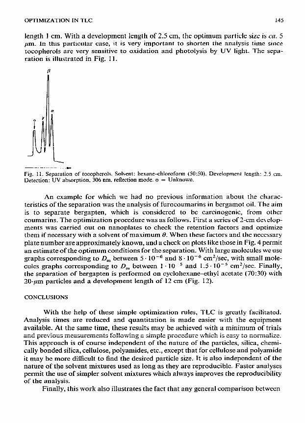
length 1 cm. With a development length of 2.5 cm, the optimum particle size is CU. 5 pm_ In this particular case, it is very important to shorten the analysis time since tocopherols are very sensitive to oxidation and photolysis by UV light. The separation is illustrated in Fig. 11.

Fig. Il. Separation of tocopherols. Solkent: henanexhloroform (5050). Development len_gth: 2.5 cm. Detection: UV absorption, 306 nm, reflection mode. o = Unknown.

An example for which we had no previous information about the characteristics of the separation was the analysis of furocoumarins in bergamot oil. The aim is to separate bergapten, which is considered to be carcinogenic, from other coumarins. The optimization procedure was as follows. First a series of Z-cm de\ elop- ments was carried out on nanoplates to check the retention factors and optimize them if necessary with a solvent of maximum 0. When these factors and the necessary plate number are approximately known, and a check on plots like those in Fig. 4 permit an estimate of the optimum conditions for the separation_ With large molecules we use graphs corresponding to D, between 5 - 10m6 and 8 - 10m6 cm’/sec, with small molecules graphs corresponding to 0, between 1 - 10 -5 and 1.5 - 10-j cm”/sec. Finally, the separation of bergapten is performed on cyclohexane-ethyl acetate (70:30) with 20-pm particles and a development length of 12 cm (Fig. 13)

CONCLUSIONS

With the help of these simple optimization rules, TLC is greatly facilitated. Analysis times are reduced and quantitation is made easier with the equipment available. At the same time, these results may be achieved with a minimum of trials and previous measurements following a simple procedure which is easy to normalize. This approach is of course independent of the nature of the particles, silica, chemi- cally bonded silica, cellulose, polyamides, etc., except that for cellulose and polyamide it may be more difficult to find the desired particle size. It is also independent of the nature of the solvent mixtures used as long as they are reproducible. Faster analyses permit the use of simpler solvent mixtures which always improves the reproducibility of the analysis.

Finally, this work also illustrates the fact that any general comparison between


Fig. 12. Separation of citropten (c) from bergapten (b) in bergamot oil. Detection: fluorescence, i.,,. 230

m, i.,. 375 nm. Development length: 12 cm on ZC-pm silica. Solvent: cyclohexane-ethyl acetate (70:30).

TLC and HPTLC is meaningless. There are cases (dyestuffs, pyrene-chrysene, chloroanilines, tocopherols) where the best results are obtained with nanoplates or TLC plates made from 5-pm particles. In other cases [bis(chlorophenyl)triazenes, aflatoxins, 2,4- and 2,5-dimethylphenols, citropten-bergapten] better performances are obtained with normal TLC plates or plates prepared from lo- or 20-pm particles. When TLC gives better performances than “high-performance TLC” this merely highlights the inadequacy of the name and that the distinction between the two techniques is irrelevant and ill-founded. In reality there is onIy one technique, which can employ a variety of materials among which the analyst has to choose the most suitable. Generally, small molecules having large diffusion coefficients are best ana- lyzed on large particles, while large molecules having small diffusion coefficients are easier to separate on plates made from small particles. However, the difficulty of the separation also has some bearing on the choice of the optimum particle size; other things being equal, difficult separations have to be carried out on coarser particles.

ACKNOWLEDGEMENTS

We are grateful to Professor I. Hal&z (Universitgt der Saarlandes, Saarbrilck- en, G.F.R.) who kindly supplied batches of classified siIica particles and to J. M. Fort& (E. Merck) for generous gifts of plates.


REFERENCES

1 E. Stahl, I. Halisz and G. Guiochon, I Irh btremariottal S~ntposiutn on Cl~romatograplty, Birtninghn, 1976.

2 G. Szekely and R. Delley, Chink, 32 (1978) 161. 3 G. Guiochon, A. Siouffi, H. En8elhardt and I. Ha&z, J. Cllronrorogr. Sci., 16 (1978) 152. 4 G. Guiochon and A. SioulIi, J. Clrronrarogr. Sci., 16 (1978) 470. 5 G. Guiochon and A. Siouffi, J. Chrotttatogr. Sri., 16 (1978) 598. 6 G. Guiachon, F. Bressolle and A. Siouffi, J. C/~~ttarogr. Sci., 17 (1979) 368. 7 E. Stahl, Die Phartm~ie, 11 (1956) 633. 8 L. R. Snyder, Principles of Adsorpfion Chromatograplz~, Marcel Dekker, New York, 1968, pp. 99-123. 9 J. H. Knox, in C. F. Simpson (Editor), Pracricd High Performance Lrquid Cizrortmtograplzy, Heyden &

Son, London, 1976, p. 19. 10 G. Vemin, La France & ses parfirms, 8 (1965) 145. I I G. Guiochon and -4. Siouffi, J. Cizromatogr. Sci., in preparation. 12 R. C. Reid and T. K. Sherwood. The Properties ofGases and Liqukk, McGraw-Hill, New York, 1958,

p_ 87. 13 E. Grushka and E. J. Kikta, Jr., J. Amer. C/rem Sot., 98 (1976) 643. 14 F. Vitiello and J.-P. Zanetta, J_ Chromatogr., 166 (1978) 637. 15 D. B. Faber. J. Clrrotwrogr., 142 (1977) 421. 16 H:Halpaap and J. Ripphahn. Chroma~ographiu, 10 (1977) 613. 17 H. Halpaap and K.-F. Krebs, J. Chrorttarogr., 142 (1977) 823. 18 M. Martin, J. Loheac and G. Guiochon, Chrottta~ographiu. 5 (1972) 33. 19 A. Siouffi, A. Guillemonat and G. Guiochon, Chromutographia, 10 (1977) 651. 20 IM. Bidlo-I@oy, J_ High Resohf. Cltrottrurogr. Chrorttarogr. Cort~ttwrt.. 1 ( 1978) 161. 11 A. Zlatkis and R. E. Kaiser (Editors), High Perfortmmce Thin-L+er Chrort~ufogrupl~~, Elsevier, Am-

sterdam, Oxford, New York, 1977. 21 J. A. Perry, J. Chromatogr.. 165 (1979) 117. 23 J. C. Touchstone and J. Sherma (Editors), Dettsirottretr_v in T/h Layer Cltmrrturogrupl~~~, Interscience,

New York, 1979, p. 707.

optimization in thin-layer chromatography : some practical considerations

Documents