optimization and mathematical programming · · 2016-04-14maximize profit = $7.00 x1 + $6.00 x2...
TRANSCRIPT

Outline
Introduction to Integer Programming (IP)
Examples of IP
Developing IP
Branch and Bound (B&B) Method
B&B Example (Minimization Problem)
B&B Example (Maximization Problem)
Solving IPs in MATLAB
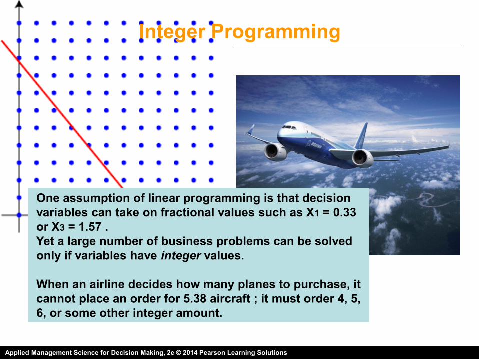
Integer Programming
One assumption of linear programming is that decision
variables can take on fractional values such as X1 = 0.33
or X3 = 1.57 .
Yet a large number of business problems can be solved
only if variables have integer values.
When an airline decides how many planes to purchase, it
cannot place an order for 5.38 aircraft ; it must order 4, 5,
6, or some other integer amount.
Applied Management Science for Decision Making, 2e © 2014 Pearson Learning Solutions

4
Introduction
Integer Programs (IP) : (NP-hard) computational complexity
Mixed Integer Linear Program (MILP) Generally (NP-hard)
However, many problems can be solved surprisingly quickly!
Philip Kilby, Australian National University, 2008

5
(Mixed) Integer Programming
• Integer Programming:
all variables must have Integer values
• Mixed Integer Programming :
some variables have integer values
Exponential solution times!
Philip Kilby, Australian National University, 2008

6
IP Examples (1)
Example IP formulation
The Knapsack problem:
I wish to select items to put in my backpack.
There are m items available.
Item i weights wi kg,
Item i has value vi.
I can carry Q kg.
otherwise0
itemselect I if1Let
ixi
1,0
s.t.
max
i
i
i
ii
ii
x
Qwx
vx
Philip Kilby, Australian National University, 2008
7
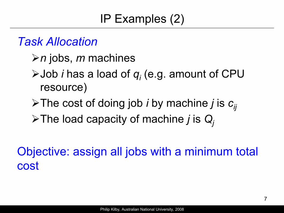
IP Examples (2)
Task Allocation
n jobs, m machines
Job i has a load of qi (e.g. amount of CPU
resource)
The cost of doing job i by machine j is cij
The load capacity of machine j is Qj
Objective: assign all jobs with a minimum total
cost
Philip Kilby, Australian National University, 2008

8
Formulation
jQqx
ix
xc
jix
i
jiij
j
ij
ji
ijij
ij
1
min
otherwise0
machine toassigned is task if1
,
Philip Kilby, Australian National University, 2008

9
Vehicle Routing Problem (VRP)
What is the optimal set of routes for a fleet of vehicles to traverse in order to deliver to a given set of customers?
• n customers and m vehicles
• ci,j – the distance or cost of travel
from i to j
• qj – load at j
• Qk – capacity of vehicle k
What vehicle should visit each customer, and in what order, to minimize costs?
If m =1 vehicle Travel Salesman Problem (TSP)
Philip Kilby, Australian National University, 2008

10
Traditional formulation
otherwise0
on vehicle precedes if1 kjixijk
...
1
c minimizekj,i,
ij
kQqx
kxx
ix
x
kj
j
ijk
i
i
ijk
j
ijk
k
ijk
j
ijk
Philip Kilby, Australian National University, 2008
11
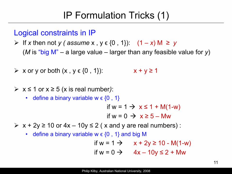
IP Formulation Tricks (1)
Logical constraints in IP
If x then not y ( assume x , y ϵ {0 , 1}): (1 – x) M ≥ y
(M is “big M” – a large value – larger than any feasible value for y)
x or y or both (x , y ϵ {0 , 1}): x + y ≥ 1
x ≤ 1 or x ≥ 5 (x is real number):
• define a binary variable w ϵ {0 , 1}
if w = 1 x ≤ 1 + M(1-w)
if w = 0 x ≥ 5 – Mw
x + 2y ≥ 10 or 4x – 10y ≤ 2 ( x and y are real numbers) :
• define a binary variable w ϵ {0 , 1} and big M
if w = 1 x + 2y ≥ 10 - M(1-w)
if w = 0 4x – 10y ≤ 2 + Mw
Philip Kilby, Australian National University, 2008

IP Formulation Tricks (2)
• For the purpose of this course, LP formulation is highly crucial. In
your homework, you will be asked to do the formulation.
• So, start learning the tricks by practice!
• Find out interesting tricks here:
http://mixedintegerprogramming.weebly.com/uploads/1/4/1/8/14181742
/integer_programming_tricks_-_aimms_modeling_guide.pdf
And here
http://ocw.mit.edu/courses/sloan-school-of-management/15-053-
optimization-methods-in-management-science-spring-2013/lecture-
notes/MIT15_053S13_lec11.pdf
12

13
Solving IPs
How can we solve IPs problems?
Philip Kilby, Australian National University, 2008

14
Solving IP
• Some problem classes have the “Integrality
Property”: all solution naturally fall on integer points
e.g.
– Maximum Flow problems
– Assignment problems
• If the constraint matrix has a special form, it will
have the Integrality Property:
– Totally unimodular
– Balanced
– Perfect
• But, not all problems have such properties
Philip Kilby, Australian National University, 2008

Solving IP by relaxing to LP
Maximize Z = 100x1 + 150x2
subject to:
8,000x1 + 4,000x2 40,000
15x1 + 30x2 200
x1, x2 0 and integer
Optimal Solution:
Z = $1,055.56
x1 = 2.22
x2 = 5.55
OBS! We get non-integer solution
Feasible Solution Space with Integer Solution Points

16
Solving IP
• How about solving LP Relaxation followed by
rounding?
-cT
x1
x2
LP Solution
Integer Solution
Philip Kilby, Australian National University, 2008

17
Solving IP
• In general, rounding does not work!
• LP solution provides lower bound (for minimization) and upper bound (for maximization) on IP
• But, rounding can be arbitrarily far away from integer solution
-cT
x1
x2
Philip Kilby, Australian National University, 2008

18
Solving IP
• Combine both approaches
Solve LP Relaxation to get fractional solutions
Create two sub-branches by adding
constraints
-cT
x1
x2
LP Solution
Integer
Solution
Philip Kilby, Australian National University, 2008

19
Solving IP
• Combine both approaches
Solve LP Relaxation to get fractional solutions
Create two sub-branches by adding
constraints
-cT
x1
x2 x1 ≥ 2
Philip Kilby, Australian National University, 2008

20
Solving IP
• Combine both approaches
Solve LP Relaxation to get fractional solutions
Create two sub-branches by adding
constraints
-cT
x1
x2
x1 ≤ 1
Philip Kilby, Australian National University, 2008
An Example Maximization Problem
21
Harrison Electric Company
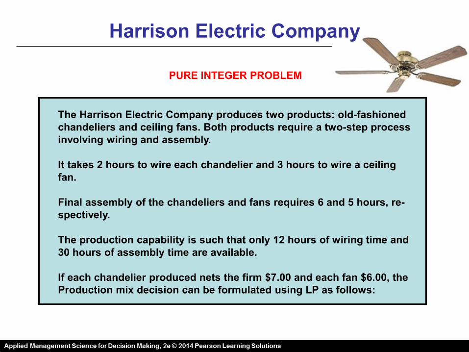
PURE INTEGER PROBLEM
The Harrison Electric Company produces two products: old-fashioned
chandeliers and ceiling fans. Both products require a two-step process
involving wiring and assembly.
It takes 2 hours to wire each chandelier and 3 hours to wire a ceiling
fan.
Final assembly of the chandeliers and fans requires 6 and 5 hours, re-
spectively.
The production capability is such that only 12 hours of wiring time and
30 hours of assembly time are available.
If each chandelier produced nets the firm $7.00 and each fan $6.00, the
Production mix decision can be formulated using LP as follows:
Harrison Electric Company
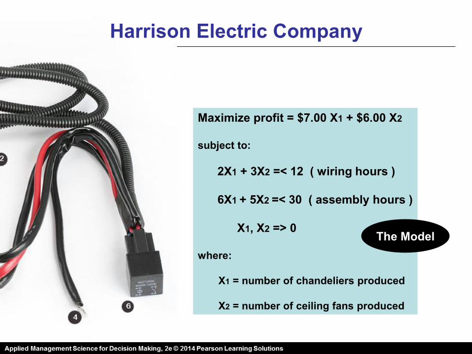
Maximize profit = $7.00 X1 + $6.00 X2
subject to:
2X1 + 3X2 =< 12 ( wiring hours )
6X1 + 5X2 =< 30 ( assembly hours )
X1, X2 => 0
where:
X1 = number of chandeliers produced
X2 = number of ceiling fans produced
The Model
Harrison Electric Company
0 1 2 3 4 5 6
6
5
4
3
2
1
0
X2
X1
+ +
+ +
+
+ +
+
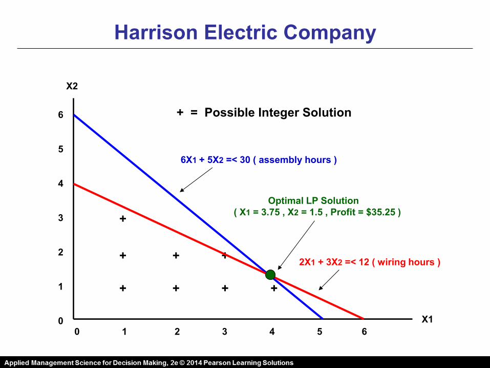
6X1 + 5X2 =< 30 ( assembly hours )
2X1 + 3X2 =< 12 ( wiring hours )
Optimal LP Solution
( X1 = 3.75 , X2 = 1.5 , Profit = $35.25 )
+ = Possible Integer Solution

Harrison Electric Company
The optimal solution is X1 = 3.75 chandeliers and X2 = 1.5 ceiling
fans.
Rounding to X1 = 4 and X2 = 2 makes the solution unfeasible.
Rounding to X1 = 4 and X2 = 2 is probably not the optimal
feasible integer solution either .
There are 18 feasible integer solutions to this problem.
The optimal integer solution is X1 = 5 and X2 = 0 , with a total
profit of $35.00 .
The integer restriction reduced profit from $35.25 to $35.00
An integer solution can never produce a greater profit than the
LP solution to the same problem.
DISCUSSION
Harrison Electric Company
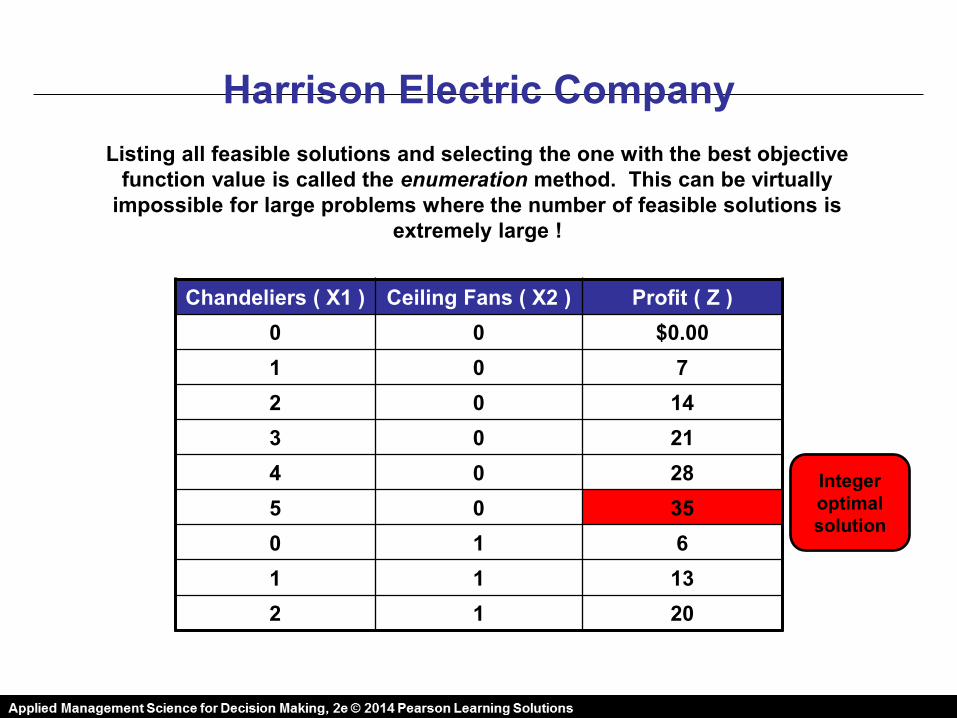
Listing all feasible solutions and selecting the one with the best objective
function value is called the enumeration method. This can be virtually
impossible for large problems where the number of feasible solutions is
extremely large !
Chandeliers ( X1 ) Ceiling Fans ( X2 ) Profit ( Z )
0 0 $0.00
1 0 7
2 0 14
3 0 21
4 0 28
5 0 35
0 1 6
1 1 13
2 1 20
Integer
optimal
solution
Harrison Electric Company
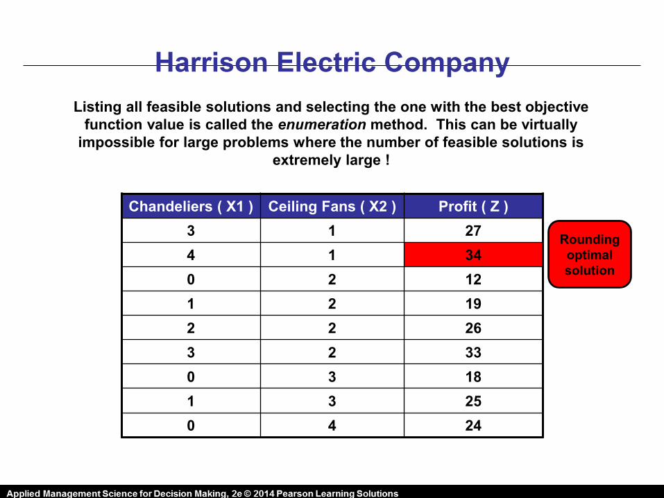
Listing all feasible solutions and selecting the one with the best objective
function value is called the enumeration method. This can be virtually
impossible for large problems where the number of feasible solutions is
extremely large !
Chandeliers ( X1 ) Ceiling Fans ( X2 ) Profit ( Z )
3 1 27
4 1 34
0 2 12
1 2 19
2 2 26
3 2 33
0 3 18
1 3 25
0 4 24
Rounding
optimal
solution

Branch-and-Bound Method
Throughout the procedure, remember that the lower bound
solution is determined by feasible integer solutions. Upper bound
is determined by fractional LP solutions. Define two parameters LB and
UB to update the lower bound and upper bound.
1. Solve the original problem using linear programming.
If the answer satisfies the integer constraints, we are
done.
If not, this value provides an initial upper bound for
the objective function.
2. Find any feasible solution that meets the integer con-
straints for use as a lower bound. Usually, rounding
down each variable will accomplish this.

Branch-and-Bound Method
3. Branch on one variable from step 1 that does not
have an integer value. Split the problem into two
subproblems based on integer values that are above
and below the noninteger value.
For example, if X2 = 3.75 was in the optimal linear
programming solution, introduce constraint X2 => 4
in the first subproblem, and X2 =< 3 in the second
subproblem.

Branch-and-Bound Method
4. Create nodes at the top of these new branches by
solving the new problems.

Branch-and-Bound Method
5. a If a branch yields a solution that is not feasible,
terminate the branch.
5. b If a branch yields a solution that is feasible, but
not an integer solution, go to step 6.
5. c If the branch yields a feasible integer solution,
look at the objective function. If its value equals
the upper bound, an optimal solution has been
reached.
If it is not equal to the upper bound, but exceeds
the lower bound, set it as the new lower bound
and go to step 6.
Finally, if it is less than the lower bound, terminate
this branch.

Branch-and-Bound Method
6. Examine both branches again and set the
upper bound equal to the maximum value
of the objective function at all final nodes.
If the upper bound equals the lower bound,
stop.
If not, go back to step 3 .

Harrison Electric Company
Maximize profit = $7.00 X1 + $6.00 X2
subject to:
2X1 + 3X2 =< 12 ( wiring hours )
6X1 + 5X2 =< 30 ( assembly hours )
X1, X2 => 0
where:
X1 = number of chandeliers produced
X2 = number of ceiling fans produced
The Model
REVISITED
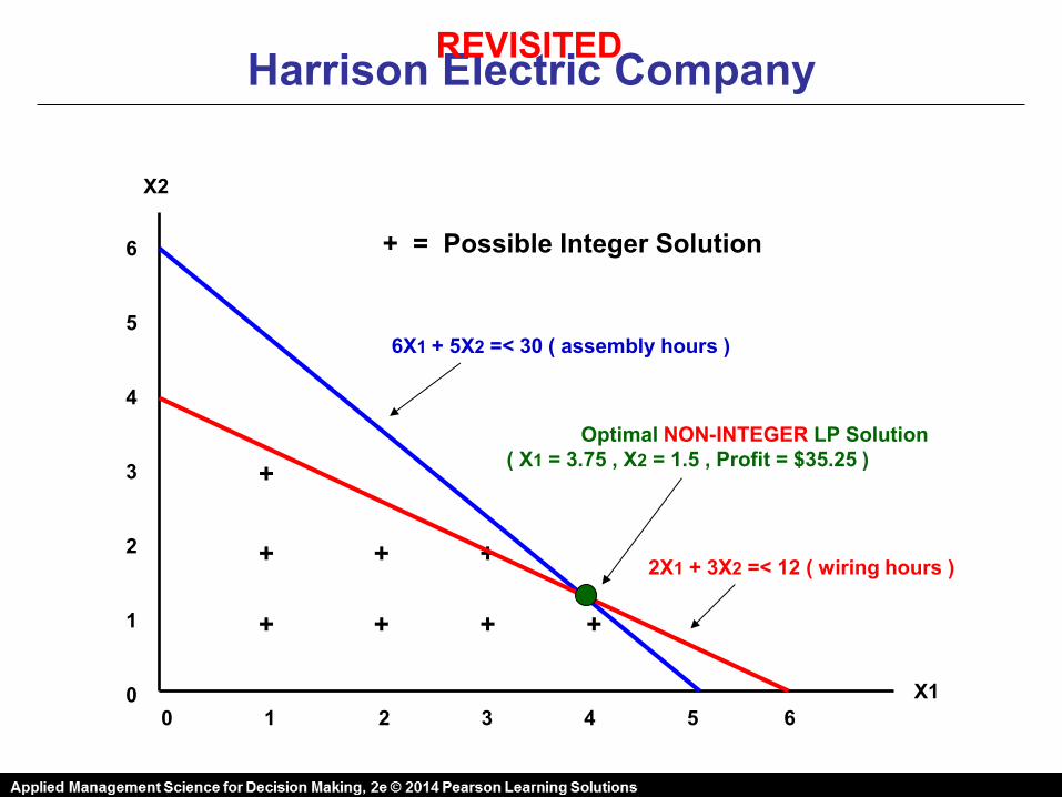
Harrison Electric Company
0 1 2 3 4 5 6
6
5
4
3
2
1
0
X2
X1
+ +
+ +
+
+ +
+
6X1 + 5X2 =< 30 ( assembly hours )
2X1 + 3X2 =< 12 ( wiring hours )
Optimal NON-INTEGER LP Solution
( X1 = 3.75 , X2 = 1.5 , Profit = $35.25 )
+ = Possible Integer Solution
REVISITED

Branch-and-Bound Method
Since X1 and X2 are not integers, the solution is not valid.
The profit of $35.25 will be the initial upper bound.
Rounding down gives X1 = 3, X2 = 1, profit = $27.00 , which
is feasible and can be used as a lower bound.
X1=3.75
X2=1.5
P=35.25
Upper Bound = $35.25
Lower Bound = $27.00
(rounding down)
Original
Non-Integer
Solution
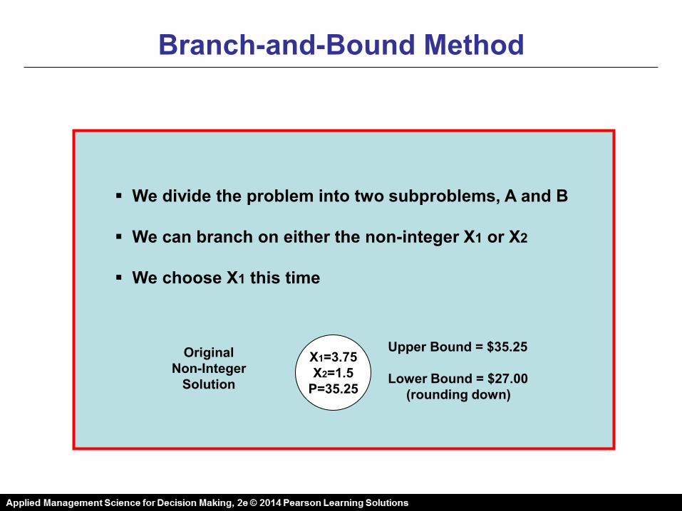
Branch-and-Bound Method
We divide the problem into two subproblems, A and B
We can branch on either the non-integer X1 or X2
We choose X1 this time
X1=3.75
X2=1.5
P=35.25
Upper Bound = $35.25
Lower Bound = $27.00
(rounding down)
Original
Non-Integer
Solution

Branch-and-Bound Method
Subproblem A
Max Z = $7X1 + $6X2
s.t. 2X1 + 3X2 =< 12
6X1 + 5X2 =< 30
X1 => 4
X1=3.75
X2=1.5
P=35.25
Upper Bound = $35.25
Lower Bound = $27.00
(rounding down)
Original
Non-Integer
Solution
Subproblem B
Max Z = $7X1 + $6X2
s.t. 2X1 + 3X2 =< 12
6X1 + 5X2 =< 30
X1 =< 3

Branch-and-Bound Method
X1=3.75
X2=1.5
P=35.25
Upper Bound = $35.25
Lower Bound = $27.00
(rounding down)
X1=4
X2=1.2
P=35.20
Subproblem A
X1=3
X2=2
P=33.00
Subproblem B
Noninteger Solution
Upper Bound = $35.20
Lower Bound = $33.00
This Branch
Solution Is Integer
New Lower Bound $33.00

Branch-and-Bound Method
Subproblem A is now branched into two new
subproblems, C and D
Subproblem C has the additional constraint of
X2 => 2
Subproblem D has the additional constraint of
X2 =< 1
The logic here is that since A’s optimal solution
of X1 = 1.2 is not feasible, the integer feasible
answer must lie at X2 => 2 or X2 =< 1

Branch-and-Bound Method
Subproblem C
Max Z = $7X1 + $6X2
s.t. 2X1 + 3X2 =< 12
6X1 + 5X2 =< 30
X1 => 4
X2 => 2
Subproblem D
Max Z = $7X1 + $6X2
s.t. 2X1 + 3X2 =< 12
6X1 + 5X2 =< 30
X1 => 4
X2 =< 1
Subproblem C has no feasible solution whatsoever because the first
two constraints are violated if X1 => 4 and X2 => 2 constraints are
observed. We terminate this branch and do not consider its solution.
Subproblem D’s solution is X1 = 4.17, X2 = 1, profit = $35.16. This non-
integer solution yields a new upper bound of $35.16.
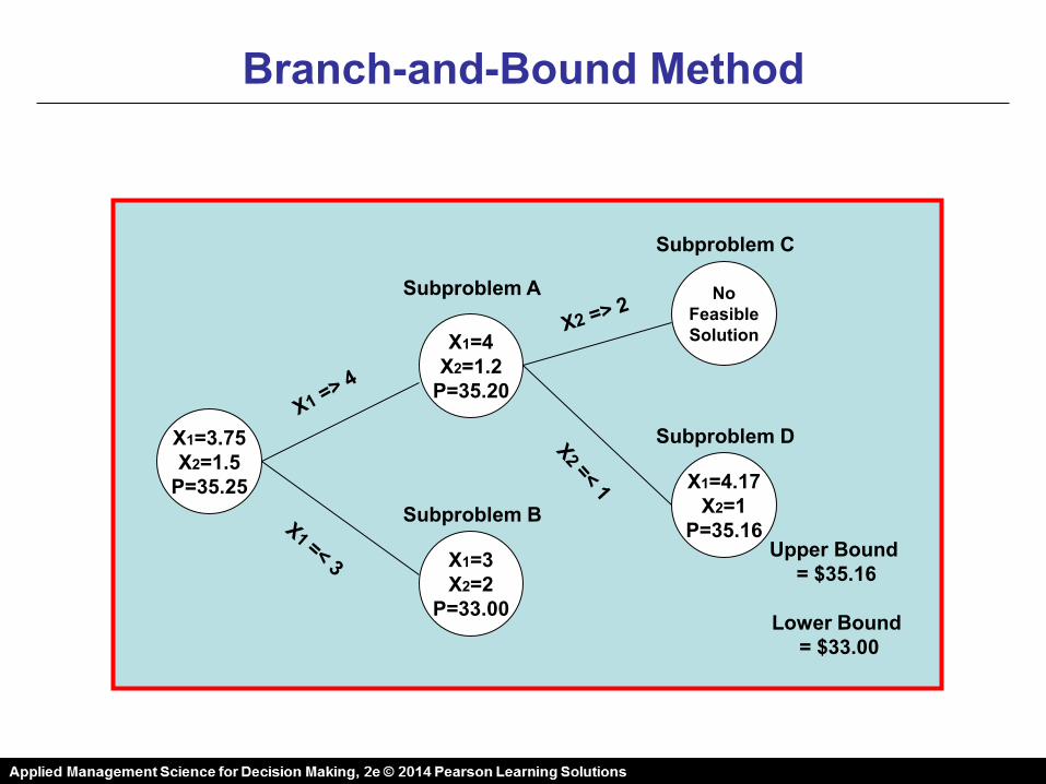
Branch-and-Bound Method
X1=3.75
X2=1.5
P=35.25
X1=4
X2=1.2
P=35.20
Subproblem A
X1=3
X2=2
P=33.00
Subproblem B
Upper Bound
= $35.16
Lower Bound
= $33.00
No
Feasible
Solution
X1=4.17
X2=1
P=35.16
Subproblem C
Subproblem D
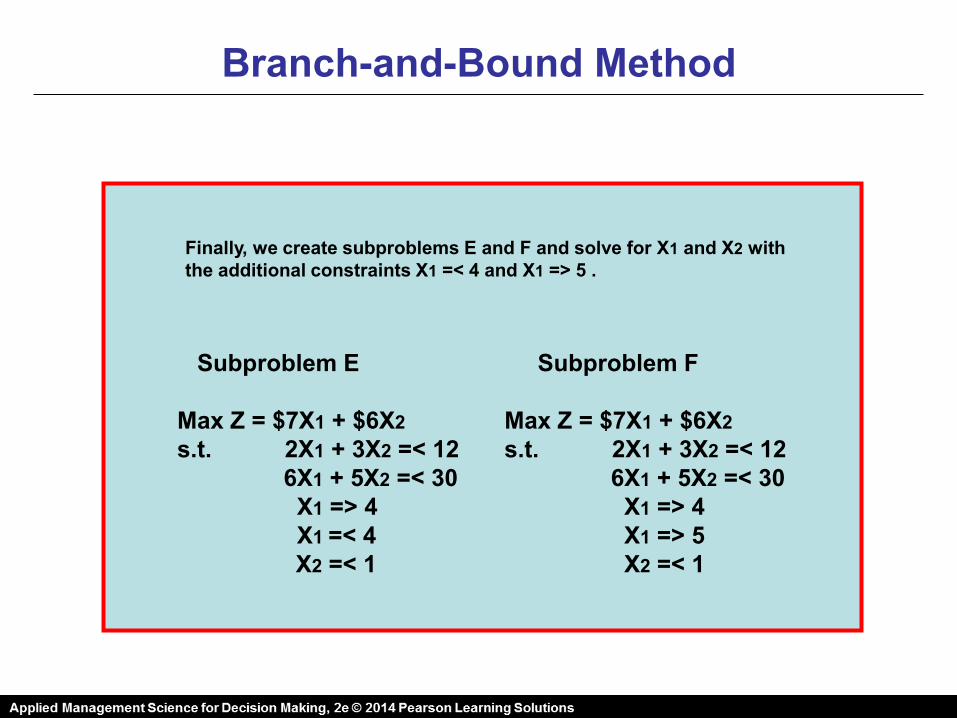
Branch-and-Bound Method
Subproblem E
Max Z = $7X1 + $6X2
s.t. 2X1 + 3X2 =< 12
6X1 + 5X2 =< 30
X1 => 4
X1 =< 4
X2 =< 1
Subproblem F
Max Z = $7X1 + $6X2
s.t. 2X1 + 3X2 =< 12
6X1 + 5X2 =< 30
X1 => 4
X1 => 5
X2 =< 1
Finally, we create subproblems E and F and solve for X1 and X2 with
the additional constraints X1 =< 4 and X1 => 5 .

Full Branch-and-Bound Solution
X1=3.75
X2=1.5
P=35.25
X1=4
X2=1.2
P=35.20
Subproblem A
X1=3
X2=2
P=33.00
Subproblem B
No
Feasible
Solution
X1=4.17
X2=1
P=35.16
Subproblem C
Subproblem D
X1=4
X2=1
P=34.00
X1=5
X2=0
P=35.00
Subproblem E
Subproblem F
Feasible
Integer
Solution
Feasible
Integer
Optimal
Solution
The stopping rule for the branching process is that we continue until the new upper
bound is less than or equal to the lower bound or no further branching is possible.
The latter is the case here since both branches yielded feasible integer solutions.
Harrison Electric Company
44
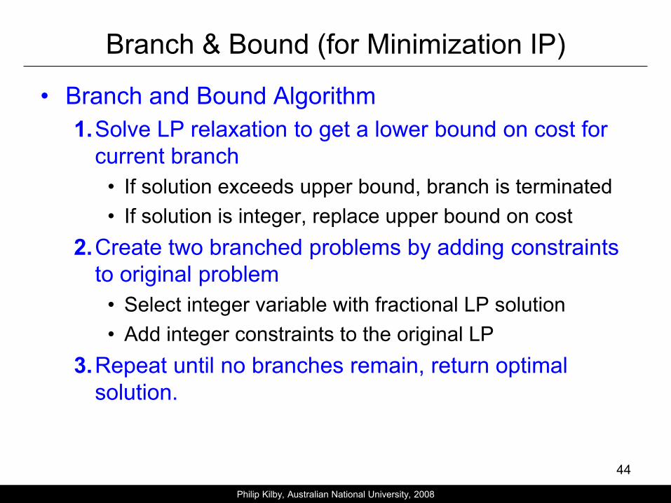
Branch & Bound (for Minimization IP)
• Branch and Bound Algorithm
1. Solve LP relaxation to get a lower bound on cost for
current branch
• If solution exceeds upper bound, branch is terminated
• If solution is integer, replace upper bound on cost
2. Create two branched problems by adding constraints
to original problem
• Select integer variable with fractional LP solution
• Add integer constraints to the original LP
3. Repeat until no branches remain, return optimal
solution.
Philip Kilby, Australian National University, 2008
An Example Minimization
Problem
45

46
Branch & Bound
• Example: a problem with 4 variables, all
required to be integer
Philip Kilby, Australian National University, 2008

47
Branch & Bound
z* = 356.1
x=(1.2,2.6,3.2,2.8) Initial LP
Philip Kilby, Australian National University, 2008
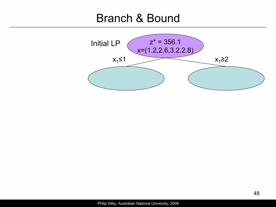
48
Branch & Bound
z* = 356.1
x=(1.2,2.6,3.2,2.8) Initial LP
x1≤1 x1≥2
Philip Kilby, Australian National University, 2008
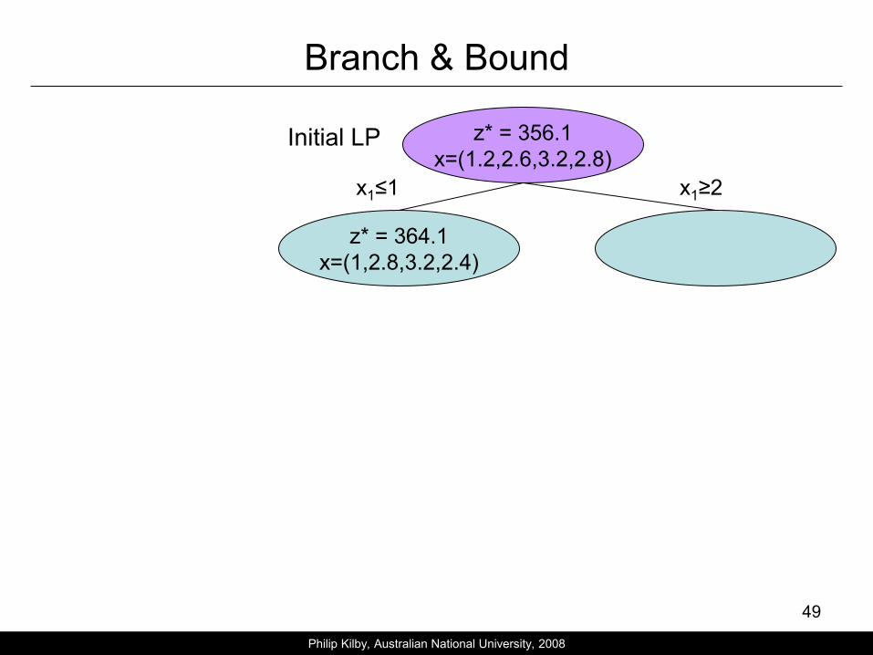
49
Branch & Bound
z* = 356.1
x=(1.2,2.6,3.2,2.8) Initial LP
z* = 364.1
x=(1,2.8,3.2,2.4)
x1≤1 x1≥2
Philip Kilby, Australian National University, 2008

50
Branch & Bound
z* = 356.1
x=(1.2,2.6,3.2,2.8) Initial LP
z* = 364.1
x=(1,2.8,3.2,2.4) z* = ∞
Infeasible
x1≤1 x1≥2
Philip Kilby, Australian National University, 2008

51
Branch & Bound
z* = 356.1
x=(1.2,2.6,3.2,2.8) Initial LP
z* = 364.1
x=(1,2.8,3.2,2.4) z* = ∞
Infeasible
x1≤1 x1≥2
Philip Kilby, Australian National University, 2008
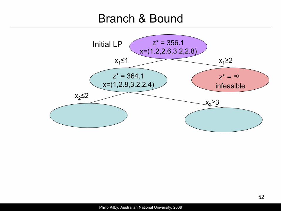
52
Branch & Bound
z* = 356.1
x=(1.2,2.6,3.2,2.8) Initial LP
z* = 364.1
x=(1,2.8,3.2,2.4) z* = ∞
infeasible
x1≤1 x1≥2
x2≤2 x2≥3
Philip Kilby, Australian National University, 2008
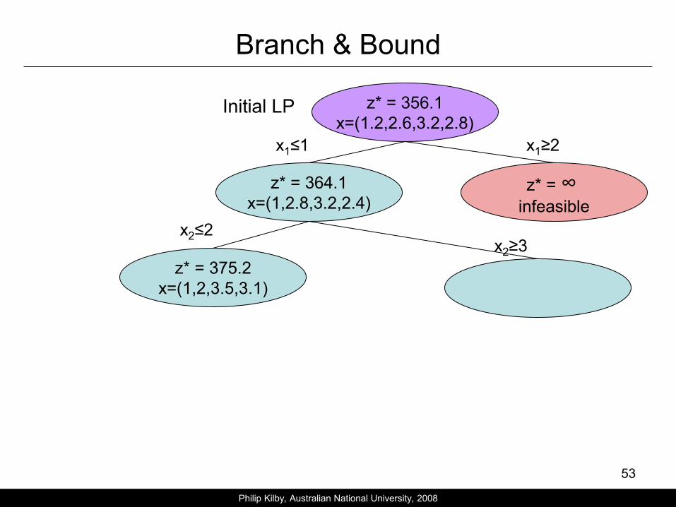
53
Branch & Bound
z* = 356.1
x=(1.2,2.6,3.2,2.8) Initial LP
z* = 364.1
x=(1,2.8,3.2,2.4) z* = ∞
infeasible
z* = 375.2
x=(1,2,3.5,3.1)
x1≤1 x1≥2
x2≤2 x2≥3
Philip Kilby, Australian National University, 2008

54
Branch & Bound
z* = 356.1
x=(1.2,2.6,3.2,2.8) Initial LP
z* = 364.1
x=(1,2.8,3.2,2.4) z* = ∞
infeasible
z* = 375.2
x=(1,2,3.5,3.1) z* = 384.1
x=(1,3,4.1,2.2)
x1≤1 x1≥2
x2≤2 x2≥3
Philip Kilby, Australian National University, 2008

55
Branch & Bound
z* = 356.1
x=(1.2,2.6,3.2,2.8) Initial LP
z* = 364.1
x=(1,2.8,3.2,2.4) z* = ∞
infeasible
z* = 375.2
x=(1,2,3.5,3.1) z* = 384.1
x=(1,3,4.1,2.2)
x1≤1 x1≥2
x2≤2 x2≥3
x3≤3 x3≥4
Philip Kilby, Australian National University, 2008

56
Branch & Bound
z* = 356.1
x=(1.2,2.6,3.2,2.8) Initial LP
z* = 364.1
x=(1,2.8,3.2,2.4) z* = ∞
infeasible
z* = 375.2
x=(1,2,3.5,3.1) z* = 384.1
x=(1,3,4.1,2.2)
z* = 380
x=(1,2,3,4)
x1≤1 x1≥2
x2≤2 x2≥3
x3≤3 x3≥4
Philip Kilby, Australian National University, 2008

57
Branch & Bound
z* = 356.1
x=(1.2,2.6,3.2,2.8) Initial LP
z* = 364.1
x=(1,2.8,3.2,2.4) z* = ∞
infeasible
z* = 375.2
x=(1,2,3.5,3.1) z* = 384.1
x=(1,3,4.1,2.2)
z* = 380
x=(1,2,3,4)
x1≤1 x1≥2
x2≤2 x2≥3
x3≤3 x3≥4
Philip Kilby, Australian National University, 2008
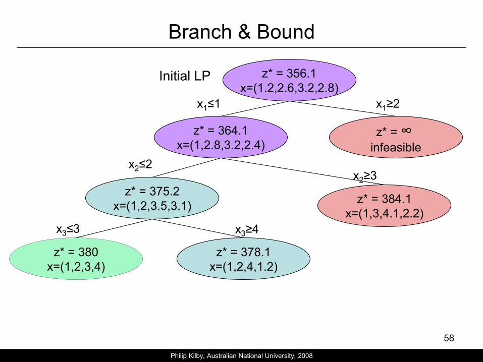
58
Branch & Bound
z* = 356.1
x=(1.2,2.6,3.2,2.8) Initial LP
z* = 364.1
x=(1,2.8,3.2,2.4) z* = ∞
infeasible
z* = 375.2
x=(1,2,3.5,3.1) z* = 384.1
x=(1,3,4.1,2.2)
z* = 380
x=(1,2,3,4)
z* = 378.1
x=(1,2,4,1.2)
x1≤1 x1≥2
x2≤2 x2≥3
x3≤3 x3≥4
Philip Kilby, Australian National University, 2008

59
Branch & Bound
z* = 356.1
x=(1.2,2.6,3.2,2.8) Initial LP
z* = 364.1
x=(1,2.8,3.2,2.4) z* = ∞
infeasible
z* = 375.2
x=(1,2,3.5,3.1) z* = 384.1
x=(1,3,4.1,2.2)
z* = 380
x=(1,2,3,4)
z* = 378.1
x=(1,2,4,1.2)
x1≤1 x1≥2
x2≤2 x2≥3
x3≤3 x3≥4
Philip Kilby, Australian National University, 2008
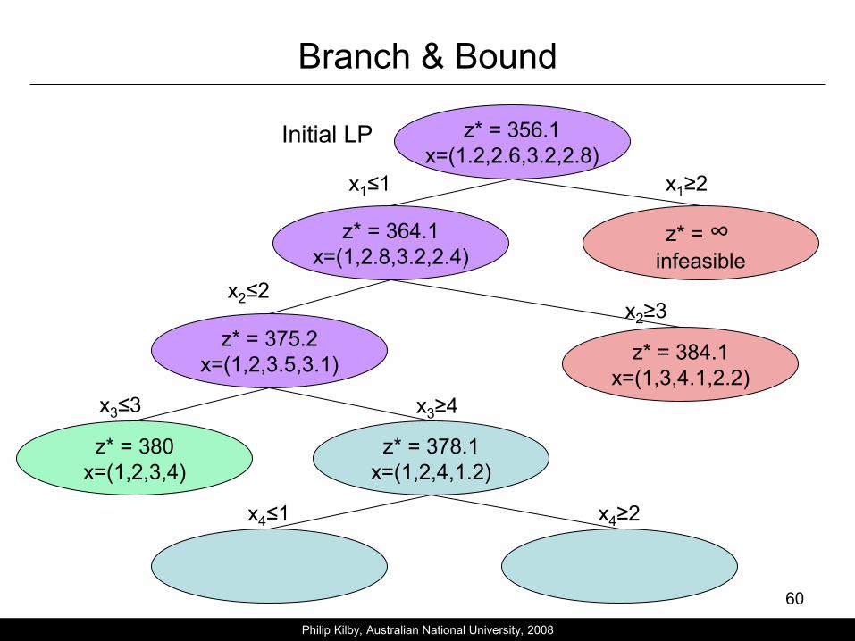
60
Branch & Bound
z* = 356.1
x=(1.2,2.6,3.2,2.8) Initial LP
z* = 364.1
x=(1,2.8,3.2,2.4) z* = ∞
infeasible
z* = 375.2
x=(1,2,3.5,3.1) z* = 384.1
x=(1,3,4.1,2.2)
z* = 380
x=(1,2,3,4)
z* = 378.1
x=(1,2,4,1.2)
x1≤1 x1≥2
x2≤2 x2≥3
x3≤3 x3≥4
x4≤1 x4≥2
Philip Kilby, Australian National University, 2008

61
Branch & Bound
z* = 356.1
x=(1.2,2.6,3.2,2.8) Initial LP
z* = 364.1
x=(1,2.8,3.2,2.4) z* = ∞
infeasible
z* = 375.2
x=(1,2,3.5,3.1) z* = 384.1
x=(1,3,4.1,2.2)
z* = 380
x=(1,2,3,4)
z* = 378.1
x=(1,2,4,1.2)
z* = 381
x=(1,2,4,0)
x1≤1 x1≥2
x2≤2 x2≥3
x3≤3 x3≥4
x4≤1 x4≥2
Philip Kilby, Australian National University, 2008

62
Branch & Bound
z* = 356.1
x=(1.2,2.6,3.2,2.8) Initial LP
z* = 364.1
x=(1,2.8,3.2,2.4) z* = ∞
infeasible
z* = 375.2
x=(1,2,3.5,3.1) z* = 384.1
x=(1,3,4.1,2.2)
z* = 380
x=(1,2,3,4)
z* = 378.1
x=(1,2,4,1.2)
z* = 381
x=(1,2,4,0)
x1≤1 x1≥2
x2≤2 x2≥3
x3≤3 x3≥4
x4≤1 x4≥2
Philip Kilby, Australian National University, 2008

63
Branch & Bound
z* = 356.1
x=(1.2,2.6,3.2,2.8) Initial LP
z* = 364.1
x=(1,2.8,3.2,2.4) z* = ∞
infeasible
z* = 375.2
x=(1,2,3.5,3.1) z* = 384.1
x=(1,3,4.1,2.2)
z* = 380
x=(1,2,3,4)
z* = 378.1
x=(1,2,4,1.2)
z* = 381
x=(1,2,4,0)
z* = 382.1
x=(1,2,4,3.3)
x1≤1 x1≥2
x2≤2 x2≥3
x3≤3 x3≥4
x4≤1 x4≥2
Philip Kilby, Australian National University, 2008
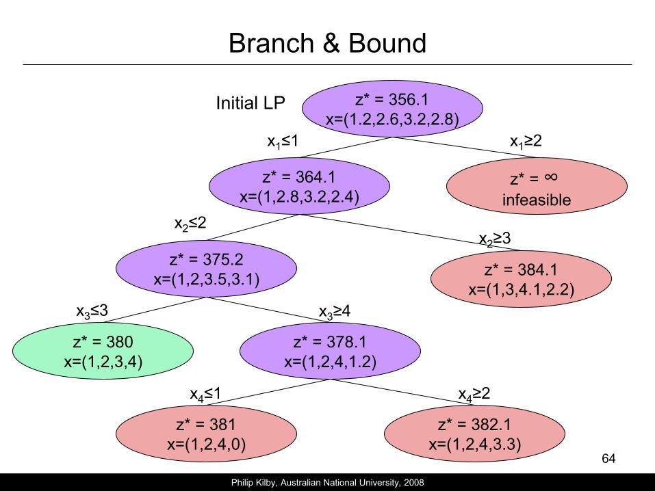
64
Branch & Bound
z* = 356.1
x=(1.2,2.6,3.2,2.8) Initial LP
z* = 364.1
x=(1,2.8,3.2,2.4) z* = ∞
infeasible
z* = 375.2
x=(1,2,3.5,3.1) z* = 384.1
x=(1,3,4.1,2.2)
z* = 380
x=(1,2,3,4)
z* = 378.1
x=(1,2,4,1.2)
z* = 381
x=(1,2,4,0)
z* = 382.1
x=(1,2,4,3.3)
x1≤1 x1≥2
x2≤2 x2≥3
x3≤3 x3≥4
x4≤1 x4≥2
Philip Kilby, Australian National University, 2008

65
Key Rules of B&B for Minimization IPs
• Each integer feasible solution is an upper
bound on solution cost,
Branching stops
It can prune other branches
Anytime result: can provide optimality bound
• Each LP-feasible solution is a lower bound on
the solution cost
Branching may stop if LB ≥ UB
Philip Kilby, Australian National University, 2008
Using Software Solvers
References
• Book:
– Integer Programming, Michele Conforti, Gérard Cornuéjols, Giacomo Zambelli
• Slides:
– Linear Programming, (Mixed) Integer Linear Programming, and Branch & Bound, Philip Kilby, Australian National University
– Integer Programming: Pure, Mixed-Integer, Zero-One Models, Applied Management Science for Decision Making, 2e © 2014 Pearson Learning Solutions