optimistic planning for the stochastic knapsack problem(2013) works with a knapsack size that...

Optimistic Planning for the Stochastic Knapsack Problem

Ciara Pike-Burke Steffen GrunewalderLancaster University Lancaster University

Abstract

The stochastic knapsack problem is astochastic resource allocation problem thatarises frequently and yet is exceptionallyhard to solve. We derive and study an op-timistic planning algorithm specifically de-signed for the stochastic knapsack problem.Unlike other optimistic planning algorithmsfor MDPs, our algorithm, OpStoK, avoids theuse of discounting and is adaptive to theamount of resources available. We achievethis behavior by means of a concentrationinequality that simultaneously applies to ca-pacity and reward estimates. Crucially, weare able to guarantee that the aforementionedconfidence regions hold collectively over alltime steps by an application of Doob’s in-equality. We demonstrate that the methodreturns an ε-optimal solution to the stochas-tic knapsack problem with high probability.To the best of our knowledge, our algorithmis the first which provides such guaranteesfor the stochastic knapsack problem. Fur-thermore, our algorithm is an anytime algo-rithm and will return a good solution evenif stopped prematurely. This is particularlyimportant given the difficulty of the prob-lem. We also provide theoretical conditionsto guarantee OpStoK does not expand all poli-cies and demonstrate favorable performancein a simple experimental setting.

1 INTRODUCTION

The stochastic knapsack problem (Dantzig, 1957), isa classic resource allocation problem that consists ofselecting a subset of items to place into a knapsack

Proceedings of the 20th International Conference on Artifi-cial Intelligence and Statistics (AISTATS) 2017, Fort Laud-erdale, Florida, USA. JMLR: W&CP volume 54. Copy-right 2017 by the author(s).

of given capacity. Placing each item in the knapsackconsumes a random amount of the capacity and pro-vides a stochastic reward. Many real world scheduling,investment, portfolio selection, and planning problemscan be formulated as the stochastic knapsack problem.Consider, for instance, a fitness app that suggests a onehour workout to a user. Each exercise (item) will takea random amount of time (size) and burn a randomamount of calories (reward). To make optimal use ofthe available time the app needs to track the progressof the user and adjust accordingly. Once an item isplaced in the knapsack, we assume we observe its re-alized size and can use this to make future decisions.This enables us to consider adaptive or closed loopstrategies, which will generally perform better (Deanet al., 2008) than open loop strategies in which theitems chosen are invariant of the remaining budget.We assume that we do not know the reward and sizedistributions of the items but are able to sample thesefrom a generative model.

Finding exact solutions to the simpler deterministicknapsack problem, in which item weights and rewardsare deterministic, is known to be NP-hard and it hasbeen stated that the stochastic knapsack problem isPSPACE-hard (Dean et al., 2008). Due to the dif-ficulty of the problem, there are currently no algo-rithms that are guaranteed to find satisfactory ap-proximations in acceptable computation time. Whileultimately one aims to have algorithms that can ap-proach large scale problems, the current state-of-the-art makes it apparent that the small scale stochasticknapsack problem must be tackled first. The emphasisin this paper is therefore on this small scale stochas-tic knapsack setting. The current state-of-the-art ap-proaches to the stochastic knapsack problem where thereward and size distributions are known, were intro-duced in Dean et al. (2008). Their algorithm splits theitems into small and large items and fills the knapsackexclusively with items of one of the two groups, ignor-ing potentially good items in the other group. Thisreturns a solution that comes within a factor of 1/(3+κ)

of the optimal, where κ > 0 is used to set a thresh-old for the small items. The strategy for small items isnon-adaptive and places items in the knapsack accord-


ing to their reward - consumption ratio. For the largeitems, a decision tree is built to some predefined depthand an exhaustive search for the best solution in thatdecision tree is performed. For most non-trivial prob-lems, this tree can be exceptionally large. The notionof small items is also underlying recent work in ma-chine learning where the reward and consumption dis-tributions are assumed to be unknown (Badanidiyuruet al., 2013). The approach in Badanidiyuru et al.(2013) works with a knapsack size that converges (in asuitable way) to infinity, rendering all items small. InBurnetas et al. (2015) adaptive strategies are consid-ered for deterministic item sizes and renewable capac-ities. The stochastic knapsack problem is also a gener-alization of the pure exploration combinatorial banditproblem Chen et al. (2014); Gabillon et al. (2016).

It is desirable to have methods for the stochastic knap-sack problem that can make use of all available re-sources and adapt to the remaining capacity. For this,the tree structure from Dean et al. (2008) can be use-ful. We propose using ideas from optimistic planning(Busoniu and Munos, 2012; Szorenyi et al., 2014) tosignificantly accelerate the tree search approach andfind adaptive strategies. Most optimistic planning al-gorithms were developed for discounted MDPs and assuch rely on discount factors to limit future rewards,effectively reducing the search tree to a tree with smalldepth. However, these discount factors are not presentin the stochastic knapsack problem. Furthermore, inour problem, the random variables representing statetransitions (item sizes) also provide us with informa-tion on the remaining capacity which relates to pos-sible future rewards. To avoid the use of discountfactors and use the transition information, we workwith confidence bounds that incorporate estimates ofthe remaining capacity. We also use these estimatesto determine how many samples we need from thegenerative model of the reward/size of an item. Forthis, we need techniques that can deal with weak de-pendencies and give confidence regions that hold si-multaneously for multiple sample sizes. We thereforecombine Doob’s martingale inequality (Doob, 1990)with Azuma-Hoeffding bounds (Azuma, 1967) to cre-ate our high probability bounds. Following the op-timistic planning approach, we use these bounds todevelop an algorithm that adapts to the complexity ofthe problem instance. In contrast to the current state-of-the-art, it is guaranteed to find an ε-good approx-imation for all problem instances and, if the probleminstance is easy to solve, it expands only a moderatesized tree. Our algorithm, OpStoK, is also an ‘anytime’algorithm in the sense that it improves rapidly to be-gin with and, even if stopped prematurely, it will stillreturn a good solution. For OpStoK, we only requireaccess to a generative model of item sizes and rewards,

and no further knowledge of the distributions.

A solution to the stochastic knapsack problem will takethe form of a policy. A policy can be thought of as asub-tree or a set of rules telling us which item to playnext depending on previous item sizes (see supplemen-tary material for examples). We define the value ofpolicy to be its expected cumulative reward and seekto find policies whose value is within ε of the optimalvalue. The performance of our algorithm is measuredin terms of the number of policies it expands in orderto find such an ε-optimal policy, since this quantity re-lates to the run-time and complexity. In practice, thenumber of policies explored by our algorithm OpStoK

is small and compares favorably to Dean et al. (2008).

1.1 Related Work

Due to the difficulty of the stochastic knapsack prob-lem, the main approximation algorithms focus on thevariant of the problem with deterministic sizes andstochastic rewards (eg. Steinberg and Parks (1979)and Morton and Wood (1998)), or stochastic sizesand deterministic rewards (eg. Dean et al. (2008) andBhalgat et al. (2011)), where the relevant distributionsare known. Of these, the most relevant to us are Deanet al. (2008) and Bhalgat et al. (2011) where decisiontrees are used to obtain approximate adaptive solu-tions. To limit the size of the decision tree, Dean et al.(2008) use a greedy strategy for ‘small’ items whileBhalgat et al. (2011) group items together. Mortonand Wood (1998) use a Monte-Carlo sampling strat-egy to generate a non-adaptive solution in the casewith stochastic rewards and deterministic sizes.

The UCT style of bandit based tree search algorithms(Kocsis and Szepesvari, 2006) uses upper confidencebounds at each node of the tree to select the best ac-tion. UCT has been shown to work in practice, how-ever, it may be too optimistic (Coquelin and Munos,2007) and theoretical results on the performance haveproved difficult to obtain. Optimistic planning wasdeveloped for tree search in large deterministic (Hrenand Munos, 2008) and stochastic systems, both open(Bubeck and Munos, 2010) and closed loop (Busoniuand Munos, 2012). The general idea is to use the upperconfidence principle of the UCB algorithm for multi-armed bandits (Auer et al., 2002) to expand a tree.This is achieved by expanding nodes that have the po-tential to lead to good solutions, by using bounds thattake into account both the reward received in gettingto a node and the reward that could be obtained aftermoving on from that node. The closest work to ours isSzorenyi et al. (2014) who use optimistic planning indiscounted MDPs, requiring only a generative modelof the rewards and transitions. Instead of the UCBalgorithm, like ours their work relies on the best arm

Ciara Pike-Burke, Steffen Grunewalder

identification algorithm of Gabillon et al. (2012).

There are several key differences between our problemand the MDPs optimistic planning algorithms are typ-ically designed for. Generally, in optimistic planningit is assumed that the state transitions do not provideany information about future reward. However, in thestochastic knapsack problem this information is rele-vant and should be taken into account when definingthe high confidence bounds. Furthermore, optimisticplanning algorithms are typically used to approximatecomplex systems at just one point and so only returna near optimal first action. In our case, the decisiontree is a good approximation to the entire problem,so we output a near-optimal policy. Furthermore, tothe best of our knowledge, our algorithm is the firstoptimistic planning algorithm to iteratively build con-fidence bounds which are used to determine whether itis necessary to sample more. One would imagine thatthe StOP algorithm from Szorenyi et al. (2014) couldbe easily adapted to the stochastic knapsack problem.However, as discussed in Section 4.1, the assumptionsrequired for this algorithm to terminate are too strongfor it to be considered feasible for this problem.

1.2 Our Contribution

Our main contributions are the anytime algo-rithm OpStoK (Algorithm 1) and subroutineBoundValueShare (Algorithm 2). These are sup-ported by the confidence bounds in Proposition 2 thatallow us to simultaneously estimate remaining capac-ity and value with guarantees that hold uniformly overmultiple sample sizes. Proposition 4 shows how wecan avoid discount based arguments and use adaptivecapacity estimates in our algorithm, and still returnan adaptive policy whose value comes within ε of theoptimal policy with high probability. Theorem 5 andCorollary 6 provide bounds on the number of samplesour algorithm uses in terms of how many policies areε-close to the best policy. The empirical performanceof OpStoK is considered in Section 7.

2 PROBLEM FORMULATION

We consider the problem of selecting a subset of itemsfrom a set, I, of K items, to place into a knapsack ofcapacity (or budget) B where each item can be playedat most once. For each item i ∈ I, let Ci and Ri benon-negative, bounded random variables defined on ajoint probability space (Ω,A, P ) which represent itssize and reward. It is assumed that we can simulatefrom the generative model of (Ri, Ci) for all i ∈ I andwe will use lower case ci and ri, to denote realiza-tions of these random variables. We assume that therandom variables (Ri, Ci) are independent of (Rj , Cj)

for all i, j ∈ I, i 6= j. Further, it is believed thatitem sizes and rewards do not change dependent on theother items in the knapsack. We assume the problemis non-trivial, in the sense that it is not possible to fitall items in the knapsack at once. If we place an itemi in the knapsack and the consumption ci is strictlygreater than the remaining capacity then we gain noreward for that item. Our final important assumptionis that there exists a known, non-decreasing functionΨ(·), satisfying limb→0 Ψ(b) = 0 and Ψ(B) <∞, suchthat the total reward that can be achieved with budgetb is upper bounded by Ψ(b). It will always be possi-ble to define such a Ψ, however, the choice of Ψ willimpact the performance of the algorithm, so we willchoose it to be as tight as possible.

Representing the stochastic knapsack problem as atree requires that all item sizes take discrete values.While in this work, it will generally be assumed thatthis is the case, in some problem instances, continu-ous item sizes need to be discretized. In this case, letξ∗ be the discretization error of the optimal policy.Then Ψ(ξ∗) is an upper bound on the extra rewardthat could be gained from the space lost due to dis-cretization. For discrete sizes, we assume there are spossible values the random variable Ci can take andthat there exists θ > 0 such that Ci ≥ θ for all i ∈ I.

2.1 Planning Trees and Policies

The stochastic knapsack problem can be thought ofas a planning tree with the initial empty state as theroot at level 0. The branches from the root representplaying an item. Similarly, each node on an even levelis an action node and its branches represent placingan item in the knapsack. The nodes on odd levelsare transition nodes with branches representing itemsizes. We define a policy Π as a finite subtree whereeach action node has at most one branch from it andeach transition node has s branches (see supplemen-tary material for examples). The depth of a policy Π,d(Π), is the number of transition nodes in any realiza-tion of the policy (where each transition node links toone branch), or equivalently, the number of items. Letd∗ = bB/θc be the maximal depth of any policy. Forany 1 ≤ d ≤ d∗, the number of policies of depth d is,

Nd =

d−1∏i=0

(K − i)si

(1)

where K = |I| is the number of items, and s the num-ber of discrete sizes.

We define a child policy, Π′, of a policy Π as a policythat follows Π up to depth d(Π) then plays additionalitems and has depth d(Π′) = d(Π) + 1. We say Π isthe parent policy of Π′. A policy Π′ is a descendant


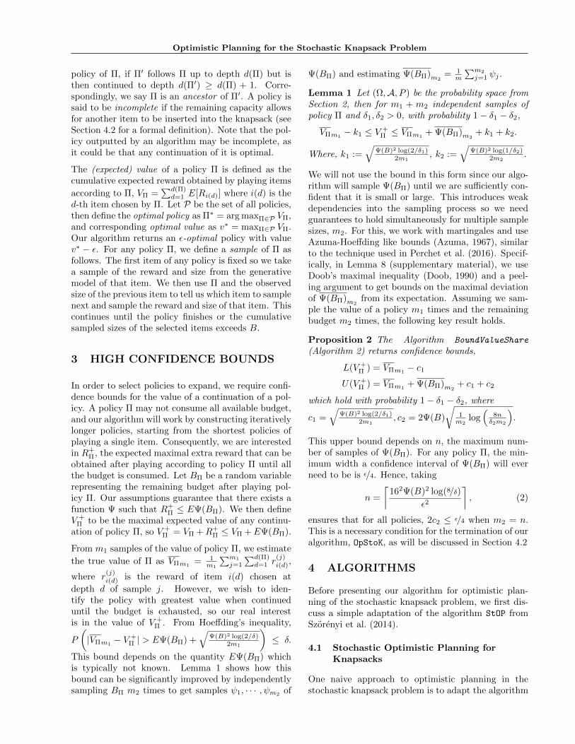
policy of Π, if Π′ follows Π up to depth d(Π) but isthen continued to depth d(Π′) ≥ d(Π) + 1. Corre-spondingly, we say Π is an ancestor of Π′. A policy issaid to be incomplete if the remaining capacity allowsfor another item to be inserted into the knapsack (seeSection 4.2 for a formal definition). Note that the pol-icy outputted by an algorithm may be incomplete, asit could be that any continuation of it is optimal.

The (expected) value of a policy Π is defined as thecumulative expected reward obtained by playing items

according to Π, VΠ =∑d(Π)d=1 E[Ri(d)] where i(d) is the

d-th item chosen by Π. Let P be the set of all policies,then define the optimal policy as Π∗ = arg maxΠ∈P VΠ,and corresponding optimal value as v∗ = maxΠ∈P VΠ.Our algorithm returns an ε-optimal policy with valuev∗ − ε. For any policy Π, we define a sample of Π asfollows. The first item of any policy is fixed so we takea sample of the reward and size from the generativemodel of that item. We then use Π and the observedsize of the previous item to tell us which item to samplenext and sample the reward and size of that item. Thiscontinues until the policy finishes or the cumulativesampled sizes of the selected items exceeds B.

3 HIGH CONFIDENCE BOUNDS

In order to select policies to expand, we require confi-dence bounds for the value of a continuation of a pol-icy. A policy Π may not consume all available budget,and our algorithm will work by constructing iterativelylonger policies, starting from the shortest policies ofplaying a single item. Consequently, we are interestedin R+

Π, the expected maximal extra reward that can beobtained after playing according to policy Π until allthe budget is consumed. Let BΠ be a random variablerepresenting the remaining budget after playing pol-icy Π. Our assumptions guarantee that there exists afunction Ψ such that R+

Π ≤ EΨ(BΠ). We then defineV +

Π to be the maximal expected value of any continu-ation of policy Π, so V +

Π = VΠ +R+Π ≤ VΠ +EΨ(BΠ).

From m1 samples of the value of policy Π, we estimate

the true value of Π as VΠm1= 1

m1

∑m1

j=1

∑d(Π)d=1 r

(j)i(d),

where r(j)i(d) is the reward of item i(d) chosen at

depth d of sample j. However, we wish to iden-tify the policy with greatest value when continueduntil the budget is exhausted, so our real interestis in the value of V +

Π . From Hoeffding’s inequality,

P

(|VΠm1

− V +Π | > EΨ(BΠ) +

√Ψ(B)2 log(2/δ)

2m1

)≤ δ.

This bound depends on the quantity EΨ(BΠ) whichis typically not known. Lemma 1 shows how thisbound can be significantly improved by independentlysampling BΠ m2 times to get samples ψ1, · · · , ψm2

of

Ψ(BΠ) and estimating Ψ(BΠ)m2= 1

m

∑m2

j=1 ψj .

Lemma 1 Let (Ω,A, P ) be the probability space fromSection 2, then for m1 + m2 independent samples ofpolicy Π and δ1, δ2 > 0, with probability 1− δ1 − δ2,

VΠm1− k1 ≤ V +

Π ≤ VΠm1+ Ψ(BΠ)m2

+ k1 + k2.

Where, k1 :=√

Ψ(B)2 log(2/δ1)2m1

, k2 :=√

Ψ(B)2 log(1/δ2)2m2

.

We will not use the bound in this form since our algo-rithm will sample Ψ(BΠ) until we are sufficiently con-fident that it is small or large. This introduces weakdependencies into the sampling process so we needguarantees to hold simultaneously for multiple samplesizes, m2. For this, we work with martingales and useAzuma-Hoeffding like bounds (Azuma, 1967), similarto the technique used in Perchet et al. (2016). Specif-ically, in Lemma 8 (supplementary material), we useDoob’s maximal inequality (Doob, 1990) and a peel-ing argument to get bounds on the maximal deviationof Ψ(BΠ)m2

from its expectation. Assuming we sam-ple the value of a policy m1 times and the remainingbudget m2 times, the following key result holds.

Proposition 2 The Algorithm BoundValueShare

(Algorithm 2) returns confidence bounds,

L(V +Π ) = VΠm1

− c1U(V +

Π ) = VΠm1+ Ψ(BΠ)m2

+ c1 + c2

which hold with probability 1− δ1 − δ2, where

c1 =√

Ψ(B)2 log(2/δ1)2m1

, c2 = 2Ψ(B)

√1m2

log(

8nδ2m2

).

This upper bound depends on n, the maximum num-ber of samples of Ψ(BΠ). For any policy Π, the min-imum width a confidence interval of Ψ(BΠ) will everneed to be is ε/4. Hence, taking

n =

⌈162Ψ(B)2 log(8/δ)

ε2

⌉, (2)

ensures that for all policies, 2c2 ≤ ε/4 when m2 = n.This is a necessary condition for the termination of ouralgorithm, OpStoK, as will be discussed in Section 4.2

4 ALGORITHMS

Before presenting our algorithm for optimistic plan-ning of the stochastic knapsack problem, we first dis-cuss a simple adaptation of the algorithm StOP fromSzorenyi et al. (2014).

4.1 Stochastic Optimistic Planning forKnapsacks

One naive approach to optimistic planning in thestochastic knapsack problem is to adapt the algorithm


StOP from Szorenyi et al. (2014). We call this adap-

tation StOP-K and replace the γd

1−γ discounting term

used to control future rewards with Ψ(B − dθ). Thisis the best upper bound on the future reward that canbe achieved without using samples of item sizes. Theupper bound on V +

Π is then VΠm + Ψ(B − dθ) + c, form samples and confidence bound c. With this, mostof the results from Szorenyi et al. (2014) follow fairlynaturally. Although StOP-K appears to be an intuitiveextension of StOP to the stochastic knapsack setting,it can be shown that for a finite number of samples,unless Ψ(B − θd∗) ≤ ε

2 , the algorithm will not ter-minate. As such, unless this restrictive assumption issatisfied StOP-K will not converge.

4.2 Optimistic Stochastic Knapsacks

In OpStoK we aim to be more efficient by only explor-ing promising policies and making better use of allinformation. In the stochastic knapsack problem, inorder to sample the value of a policy, we must sampleitem sizes to decide which item to play next. We pro-pose to make better use of these samples by calculatingU(Ψ(BΠ)) from the item size samples, and then incor-porating this into U(V +

Π ). We also pool samples of thereward and size of items across policies, thus reducingthe number of calls to the generative model. OpStoK

benefits from an adaptive sampling scheme that re-duces sample complexity and ensures that an entireε-optimal policy is returned when the algorithm stops.The performance of this sampling strategy is guaran-teed by Proposition 2.

In the main algorithm, OpStoK (Algorithm 1) is verysimilar to StOP-K Szorenyi et al. (2014) with thekey differences appearing in the sampling and con-struction of confidence bounds which are defined inBoundValueShare (Algorithm 2). The general in-tuition is that only promising policies are explored.OpStoK maintains a set of ‘active’ policies. As inSzorenyi et al. (2014) and Gabillon et al. (2012), ateach time step t, a policy, Πt to expand is chosen bycomparing the upper confidence bounds of the two bestactive policies. We select the policy with most uncer-tainty in the bounds since we want our estimates ofthe near-optimal policies to be such that we can con-fidently conclude that the policy we output is better(see Figure 5, supplementary material). Once we haveselected a policy, Πt, if the stopping criteria in Line 12is not met, we replace Πt in the set of active policieswith all its children. We refer to this as expanding apolicy. For each child policy, Π′, we bound its valueusing BoundValueShare with parameters

δd(Π′),1 =δ0,1d∗

N−1d(Π′) and, δd(Π′),2 =

δ0,2d∗

N−1d(Π′) (3)

where Nd is the number of policies of depth d as givenin (1). This ensures that all our bounds to hold simul-taneously with probability greater than 1− δ0,1 − δ0,2(as shown in Lemma 12, supplementary material).The algorithm stops in Line 12 and returns a policyΠ∗ if L(V +

Π∗) + ε ≥ maxΠ∈Active\Π∗ U(V +Π ) and we

can be confident Π∗ is within ε of optimal. OpStoK

relies on BoundValueShare (Algorithm 2) and sub-routines, EstimateValue and SampleBudget (Algo-rithms 3 and 4, supplementary material), which sam-ple the value and budget of policies.

In BoundValueShare, we use samples of both item sizeand reward to bound the value of a policy. We defineupper and lower bounds on the value of any extensionof a policy Π as,

U(V +Π ) = VΠm1

+ Ψ(BΠ)m2+ c1 + c2,

L(V +Π ) = VΠm1

− c1,

with c1 and c2 as in Proposition 2. It is also possi-ble to define upper and lower bounds on Ψ(BΠ) withm2 samples and confidence δ2. From this, we canformally define a complete policy as a policy Π withU(BΠ) = Ψ(BΠ)m2

+ c2 ≤ ε2 . For complete policies,

since there is very little capacity left, it is more im-portant to get tight confidence bounds on the valueof the policy. Hence, in BoundValueShare, we samplethe remaining budget of a policy as much as is nec-essary to conclude whether the policy is complete ornot. As soon as we realize we have a complete policy(U(BΠ) ≤ ε/2), we sample the value of that policy suf-ficiently to get a confidence interval on V +

Π of widthless than ε. Then, when it comes to choosing an op-timal policy to return, the confidence intervals of allcomplete policies will be narrow enough for this tohappen. This is appropriate since pre-specifying thenumber of samples may not lead to confidence boundstight enough to select an ε-optimal policy. Further-more, we focus sampling efforts only on promising poli-cies that are near completion. If a complete policy is

chosen as Π(1)t in OpStoK, for some t, the algorithm will

stop and this policy will be returned. For this to hap-pen, we check the stopping criterion before selectinga policy to expand. Note that in BoundValueShare,the value and remaining budget of a policy must besampled separately as we are considering closed-loopplanning so the item chosen may depend on the size ofthe previous item, and hence the value will depend onthe instantiated item sizes. For an incomplete policy,the number of samples of the value, m1, is defined toensure that the uncertainty in the estimate of VΠ isless than u(Ψ(BΠ)) = minU(Ψ(BΠ)),Ψ(B), since amaximal upper bound for the value of Π is Ψ(B).

Since at each time step OpStoK expands the policy withbest or second best upper confidence bound, the policy


Algorithm 1: OpStoK (I, δ0,1, δ0,2, ε)

Initialization: Active = ∅.1 for all i ∈ I do2 Πi = policy consisting of just playing item i;3 d(Πi) = 1;

4 δ1,1 =δ0,1d∗ N

−11 , δ1,2 =

δ0,2d∗ N

−11 ;

5 (L(V +Πi

), U(V +Πi

)) = BoundValueShare

(Πi, δ1,1, δ1,2,S∗, ε);6 Active = Active ∪ Πi;7 end8 for t = 1, 2, . . . do

9 Π(1)t = arg maxΠ∈Active U(V +

Π );

10 Π(2)t = arg max

Π∈Active\Π(1)t

U(V +Π );

11 if L(V +

Π(1)t

) + ε ≥ U(V +

Π(2)t

) then

12 Stop: Π∗ = Π(1)t ;

13 a∗ = arg maxa∈1,2 U(Ψ(BΠ

(a)t

));

14 Πt = Π(a∗)t ;

15 Active = Active \ Πt16 for all children Π′ of Πt do17 d(Π′) = d(Πt) + 1;

18 δd(Π′),1 =δ0,1d∗ N

−1d(Π′), δd(Π′),2 =

δ0,2d∗ N

−1d(Π′)

19 (L(V +Π′), U(V +

Π′)) = BoundValueShare

(Π′, δd(Π′),1, δd(Π′),2,S∗, ε);20 Active = Active ∪ Π′;21 end

22 end

it expands will always have the potential to be opti-mal. Therefore, if the algorithm is stopped before thetermination criteria is met and the active policy withbest estimated value is selected, this policy will be thebest of those with the potential to be optimal that havealready been explored. Hence, it will be a good policy(or beginning of policy). OpStoK considerably reducesthe number of calls to the generative model by creatingsets S∗i of samples of the reward and size of each itemi ∈ I. When it is necessary to sample the reward andsize of an item, i, for the evaluation of a policy, we sam-ple without replacement from S∗i until |S∗i | sampleshave been taken. At this point new calls to the gener-ative model are made and the new samples added tothe sets for use by future policies. This is illustrated inEstimateValue and SampleBudget(Algorithms 3 and4, supplementary material). We denote by S∗ the col-lection of all sets S∗i .

5 ε-CRITICAL POLICIES

The set of ε-critical policies associated with an algo-rithm is the set of all policies the algorithm may poten-

Algorithm 2: BoundValueShare(Π, δ1, δ2, S∗, ε)

Initialization: For all i ∈ I, Si = S∗i .

1 Set m2 = 1 and (ψ1,S) = SampleBudget(Π,S);

/* sample the remaining budget */

2 Ψ(BΠ)m2= 1

m2

∑m2

j=1 ψj ;

3 U(Ψ(BΠ)) = Ψ(BΠ)m2+ 2Ψ(B)

√1m2

log(

8nδm2

),

L(Ψ(BΠ)) = Ψ(BΠ)m2− 2Ψ(B)

√1m2

log(

8nδm2

);

/* calculate bounds on Ψ(BΠ) */

4 if U(Ψ(BΠ)) ≤ ε2 then

m1 =⌈

8Ψ(B)2 log(2/δ1)ε2

⌉;;

5 else if L(Ψ(BΠ)) ≥ ε4 then

6 m1 =⌈

12

Ψ(B)2 log(2/δ1)u(Ψ(BΠ))2

⌉;

7 else

8 Set m2 = m2 + 1;

9 (ψm2,S) = SampleBudget(Π,S) and go to 2

10 VΠm1= EstimateValue(Π,m1);

11 L(V +Π ) = VΠm1

−√

Ψ(B)2 log(2/δ1)2m1

;

12 U(V +Π ) = VΠm1

+ Ψ(BΠ)m2+√

Ψ(B)2 log(2/δ1)2m1

+2Ψ(B)

√1m2

log(

8nδm2

);

13 return (L(V +Π ), U(V +

Π ))

tially expand in order to obtain an ε-optimal solution.Hence, the number of ε-critical policies represents abound on the number of policies an algorithm mayexplore in order to obtain this ε-optimal solution.

To define the set of ε-critical policies associated withOpStoK, let

QεIC = Π;VΠ + 6EΨ(BΠ)− 3ε/4 ≥ v∗

−6EΨ(BΠ) + 3ε/4 + εand QεC = Π;VΠ + ε ≥ v∗ ,

represent the set of potentially optimal incomplete andcomplete policies. The set of all ε-critical policies isthen Qε = QεIC

⋃QεC . The following lemma shows

that all policies expanded by OpStoK are in Qε.

Lemma 3 Assume that L(V +Π ) ≤ VΠ ≤ U(V +

Π )holds simultaneously for all policies Π ∈ Active withU(V +

Π ) and L(V +Π ) as defined in Proposition 2. Then,

Πt ∈ Qε for every policy, Πt, selected by OpStoK atevery time point t, except for possibly the last one.

We now turn to demonstrating that under certain con-


ditions, OpStoK will not expand all policies (althoughin practice this claim should hold even when some ofthe assumptions are violated). From considering thedefinition of QεIC from Section 6, it can be shown thatif there exists a subset I ′ of items and λ > 0 satisfying,∑

i∈I′E[Ri] < v∗ − ε, and,

E

[Ψ

(B −

∑i∈I′

Ci

)]<

5ε

24+

λ

12

(4)

then QεIC is a proper subset of all incomplete policiesand as such, not all incomplete policies will need tobe evaluated by OpStoK. Furthermore, since any pol-icy of depth d > 1 will only be evaluated by OpStoK

if a descendant of it has previously been evaluated, itfollows that a complete policy in QεC must have an in-complete descendant in QεIC . Therefore, since QεIC isnot equal to the set of all incomplete policies, QεC willalso be a proper subset of all complete policies and soQε ( P. Note that the bounds used to obtain theseconditions are worst case as they involve assuming thetrue value of Ψ(BΠ) lies at one extreme of the confi-dence interval. Hence, even if the conditions in (4) arenot satisfied, it is unlikely that OpStoK will evaluateall policies. However, the conditions in (4) are easilysatisfied. Consider, for example, the problem instancewhere ε = 0.05,Ψ(b) = b ∀0 ≤ b ≤ B, v∗ = 1 andB = 1. Assume there are 3 items i1, i2, i3 ∈ I withE[Ri] < 1/8 and E[Ci] = 8/25. Then if I ′ = i1, i2, i3and λ = 5/8, the conditions of (4) are satisfied andOpStoK will not evaluate all policies.

6 ANALYSIS

In this section we give theoretical guarantees on theperformance of OpStoK, with the proofs of all resultsin the supplementary material. We begin with theconsistency result:

Proposition 4 With probability at least (1 − δ0,1 −δ0,2), the algorithm OpStoK returns a policy with valueat least v∗ − ε for ε > 0.

To obtain a bound on the sample complexity ofOpStoK, we return to the definition of ε-critical policiesfrom Section 5. The set of ε-critical policies, Qε, canbe represented as the union of three disjoint sets, Qε =Aε∪Bε∪Cε, as illustrated in Figure 1 where Aε = Π ∈Qε|EΨ(BΠ) ≤ ε/4,Bε = Π ∈ Qε|EΨ(BΠ) ≥ ε/2 andCε = Π ∈ Qε|ε/4 < EΨ(BΠ) < ε/2. Using this, inTheorem 5 the total number of samples of item size orreward required by OpStoK can be bounded as follows.

Theorem 5 With probability greater than 1−δ0,2, thetotal number of samples required by OpStoK is bounded

ε2

ε4

Case 1 Case 2 Case 3

Ψ(BΠ)

Figure 1: The three possible cases of EΨ(BΠ). Inthe first case, EΨ(BΠ) ≤ ε

4 so Π ∈ Aε, in the secondcase EΨ(BΠ) ≥ ε

2 so Π ∈ Bε, and in the final caseε4 < EΨ(BΠ) < ε

2 so Π ∈ Cε.

from above by,∑Π∈Qε

(m1(Π) +m2(Π)) d(Π).

Where, for Π ∈ Aε,m1(Π) =⌈

8Ψ(B)2 log( 2δd(Π),1

)/ε2⌉,

for Π ∈ Bε,m1(Π) ≤⌈

Ψ(B)2 log( 2δd(Π),1

)/2EΨ(BΠ)2⌉,

and for Π ∈ Cε,m1(Π) ≤ max⌈

8Ψ(B)2 log( 2δd(Π),1

)/ε2⌉,⌈

2Ψ(B)2 log( 2δd,1

)/EΨ(BΠ)2⌉.

And m2(Π) = m∗, where m∗ is the smallest integersatisfying,

32Ψ(B)2/(EΨ(BΠ)−ε/2)2 ≤ m/log(4n/mδ2) for Π ∈ Aε,

32Ψ(B)2/(EΨ(BΠ)−ε/4)2 ≤ m/log(4n/mδ2) for Π ∈ Bε,

32Ψ(B)2/(ε/4)2 ≤ m/log(4n/mδ2) for Π ∈ Cε.

We now bound the number of calls to the genera-tive model required by OpStoK. We consider the ex-pected number of times item i needs to be sampledby a policy Π. Let i1, . . . , iq denote the q nodes inpolicy Π where item i is played. Then for each nodeik(1 ≤ k ≤ q), denote by ζik the unique route to nodeik. Define d(ζik) to be the depth of node ik, or thenumber of items played along route ζik . Then theprobability of reaching node ik (or taking route ζik) is

P (ζik) =∏d(ζik )

`=1 p`,Π(ik,`), where ik,` denotes the `thitem on the route to node ik and pl,Π(i) is the probabil-ity of playing item i at depth l of policy Π for given sizedistributions. Denote the probability of playing item iin policy Π by PΠ(i), then PΠ(i) =

∑qk=1 P (ζik). Us-

ing this, the expected number of samples of the rewardand size of item i required by policy Π are less thanm1(Π)PΠ(i) and m2(Π)PΠ(i), respectively. Since sam-ples are shared between policies, the expected numberof calls to the generative model of item i is as givenbelow and used in Corollary 6,

M(i) ≤ maxΠ∈Qε

maxm1(Π)PΠ(i),m2(Π)PΠ(i)

.


Figure 2: Item sizes and rewards. Each color is anitem with horizontal lines between the two sizes andvertical lines between minimum and maximum reward.The lines cross at the point (mean size, mean reward).

Corollary 6 The expected total number of calls to thegenerative model by OpStoK for a stochastic knapsack

problem of K items is less than or equal to∑Ki=1M(i).

7 EXPERIMENTAL RESULTS

We demonstrate the performance of OpStoK on a sim-ple experimental setup with 6 items. Each item i cantake two sizes and is larger with probability xi. The re-wards come from scaled and shifted Beta distributions.The budget is 7 meaning that a maximum of 3 itemscan be placed in the knapsack. We take Ψ(b) = b andset the parameters of the algorithm to δ0,1 = δ0,2 = 0.1and ε = 0.5. Figure 2 illustrates the problem.

We compare the performance of OpStoK in this set-ting to the algorithm in Dean et al. (2008) run withvarious values of κ, the parameter used to define thesmall items threshold. We chose κ to ensure that weconsider all cases from 0 small items to 6 small items.Note that the algorithm in Dean et al. (2008) is de-signed for deterministic rewards so we sampled the re-wards for each item at the start to get estimates ofthe true rewards. When sampling item sizes for Deanet al. (2008), we used the OpStoK sampling strategy.For both algorithms, when evaluating the value of apolicy, we re-sampled the value of the chosen policiesas discussed in Section 2.1. The results of this exper-iment are shown in Figure 3. From this, the anytimeproperty of our algorithm can be seen; it is able tofind a good policy early on (after less than 100 poli-cies) so if it was stopped early, it would still returna policy with a high expected value. Furthermore, attermination, the algorithm has almost reached the bestsolution from Dean et al. (2008) which required morethan twice as many policies to be evaluated. Thus thisexperiment has shown that our algorithm not only re-turns a policy with near optimal value, but it does thisafter evaluating significantly fewer policies and, even

Figure 3: Num policies vs value. The blue line isthe estimated value of the best policy so far found byOpStoK which terminates at the square. The green di-amonds are the best value for Dean et al. (2008) whensmall items are chosen, and red circles when it chooseslarge items. The estimated value of the best solutionfrom Dean et al. (2008) is given by the red dashed line.

if stopped prematurely, it will return a good policy.

These experimental results were obtained using theOpStoK algorithm as stated in Algorithm 1. This al-gorithm incorporates the sharing of samples betweenpolicies and preferential sampling of complete policiesto improve performance. For large problems, the com-putational performance of OpStoK can be further im-proved by parallelization. In particular, the expansionof a policy can be done in parallel with each leaf of thepolicy being expanded on a different core and then re-combined. It is also possible to sample the value andremaining budget of a policy in parallel.

8 CONCLUSION

In this paper we have presented OpStoK, a new anytimeoptimistic planning algorithm specifically tailored tothe stochastic knapsack problem. For this algorithm,we have provided confidence intervals, consistency re-sults, bounds on the sample size and shown that itneedn’t evaluate all policies to find an ε-optimal solu-tion; making it the first such algorithm for the stochas-tic knapsack problem. By using estimates of the re-maining budget and value, OpStoK is adaptive and alsobenefits from a unique streamlined sampling scheme.While OpStoK was developed for the stochastic knap-sack problem, it is hoped that it is just the first steptowards using optimistic planning to tackle many fre-quently occurring resource allocation problems.

Acknowledgments

We are grateful for the support of the EPSRC fundedEP/L015692/1 STOR-i centre for doctoral trainingand Sparx.


References

P. Auer, N. Cesa-Bianchi, and P. Fischer. Finite-timeanalysis of the multiarmed bandit problem. MachineLearning, 47(2-3):235–256, 2002.

K. Azuma. Weighted sums of certain dependent ran-dom variables. Tohoku Mathematical Journal, Sec-ond Series, 19(3):357–367, 1967.

A. Badanidiyuru, R. Kleinberg, and A. Slivkins. Ban-dits with knapsacks. In IEEE 54th Annual Sympo-sium on Foundations of Computer Science, 2013.

A. Bhalgat, A. Goel, and S. Khanna. Improved ap-proximation results for stochastic knapsack prob-lems. In Twenty-Second Annual ACM-SIAM Sym-posium on Discrete Algorithms, pages 1647–1665.SIAM, 2011.

S. Bubeck and R. Munos. Open loop optimistic plan-ning. In Conference on Learning Theory, pages 477–489, 2010.

A. N. Burnetas, O. Kanavetas, and M. N. Kate-hakis. Asymptotically optimal multi-armed ban-dit policies under a cost constraint. arXiv preprintarXiv:1509.02857, 2015.

L. Busoniu and R. Munos. Optimistic planning formarkov decision processes. In 15th InternationalConference on Artificial Intelligence and Statistics,pages 182–189, 2012.

S. Chen, T. Lin, I. King, M. R. Lyu, and W. Chen.Combinatorial pure exploration of multi-armed ban-dits. In Advances in Neural Information ProcessingSystems, pages 379–387, 2014.

P.-A. Coquelin and R. Munos. Bandit algorithms fortree search. In Twenty-Third Conference on Uncer-tainty in Artificial Intelligence, pages 67–74, 2007.

G. B. Dantzig. Discrete-variable extremum problems.Operations Research, 5(2):266–288, 1957.

B. C. Dean, M. X. Goemans, and J. Vondrak. Ap-proximating the stochastic knapsack problem: Thebenefit of adaptivity. Mathematics of Operations Re-search, 33(4):945–964, 2008.

J. L. Doob. Stochastic processes. 1990.

V. Gabillon, M. Ghavamzadeh, and A. Lazaric. Bestarm identification: A unified approach to fixed bud-get and fixed confidence. In Advances in NeuralInformation Processing Systems, pages 3212–3220,2012.

V. Gabillon, A. Lazaric, M. Ghavamzadeh, R. Ortner,and P. Barlett. Improved learning complexity incombinatorial pure exploration bandits. In 19th In-ternational Conference on Artificial Intelligence andStatistics, pages 1004–1012, 2016.

J.-F. Hren and R. Munos. Optimistic planning of de-terministic systems. In European Workshop on Re-inforcement Learning, pages 151–164, 2008.

L. Kocsis and C. Szepesvari. Bandit based monte-carlo planning. In European Conference on MachineLearning, pages 282–293. 2006.

D. P. Morton and R. K. Wood. On a stochasticknapsack problem and generalizations. In Advancesin computational and stochastic optimization, logicprogramming, and heuristic search, pages 149–168.Springer, 1998.

V. Perchet, P. Rigollet, S. Chassang, and E. Snowberg.Batched bandit problems. The Annals of Statistics,44(2):660–681, 2016.

E. Steinberg and M. Parks. A preference orderdynamic program for a knapsack problem withstochastic rewards. Journal of the Operational Re-search Society, pages 141–147, 1979.

B. Szorenyi, G. Kedenburg, and R. Munos. Optimisticplanning in markov decision processes using a gen-erative model. In Advances in Neural InformationProcessing Systems, pages 1035–1043, 2014.

D. Williams. Probability with martingales. Cambridgeuniversity press, 1991.


Supplementary Material

A Illustration of Policies

(a) A policy of just playing item 3. This policy hasdepth 1.

(b) A policy that plays item 2 first. If it is small, itplays item 1 whereas if it is large it plays item 3. Afterthis, the final item is determined due to the fact thatthere are only 3 items in the problem. This policy hasdepth 2.

Figure 4: Examples of policies in the simple 3 item, 2 sizes stochastic knapsack problem. Each blue line representschoosing an item and the red lines represent the sizes of the previous items.

B Illustration of Bounds

U(VΠ)

VΠ

L(VΠ)

U(V ∗Π)

v∗

L(V ∗Π)

Figure 5: Example of where just looking at the optimistic policy might fail: If we always play the optimisticpolicy then, since U(V +

Π∗) ≥ U(V +Π ), we will always play Π∗ and so the confidence bounds on Π will not shrink.

This means that L(V +Π∗) will never be (epsilon) greater than the best alternative upper bound so there will not

be enough confidence to conclude we have found the best policy.

C Algorithms

In these algorithms Generate(i) samples a reward and item size pair from the generative model of item i, whereassample(A, k) samples from a set A with replacement to get k samples. The notation i(d) = Π(d, b) indicatesthat item i(d) was chosen by policy Π at depth d when the remaining capacity was b.


Algorithm 3: EstimateValue(Π,m)

Initialization: For all i ∈ I, Si = S∗i1 for j = 1, . . . ,m do2 B0 = B;3 for d = 1, . . . , d(Π) do4 i(d) = Π(d,Bd−1);5 if |Si(d)! ≤ 0 then (ri(d), ci(d)) = Generate(i(d)), S∗i = S∗i ∪ ri(d), ci(d));6 else (ri(d), ci(d)) = sample(Si, 1), and Si = Si \ (ri(d), ci(d));7 Bd = Bd−1 − ci(d);8 if Bd < 0 then ri(d) = 0;

9 end

10 VΠ(j)

=∑d(Π)d=1 ri(d);

11 end

12 return (VΠm = 1m

∑mj=1 VΠ

(j),S∗)

Algorithm 4: SampleBudget(Π,S)

Initialization: B0 = B and for all i ∈ I, Si = S∗i1 for d = 1, . . . , d(Π) do2 i(d) = Π(d,Bd−1);3 if |Si(d)| ≤ 0 then (ri(d), ci(d)) = Generate(i(d)), S∗i = S∗i ∪ ri(d), ci(d));4 else (ri(d), ci(d)) = sample(Si, 1), and Si = Si \ (ri(d), ci(d));5 Bd = Bd−1 − ci(d);

6 end

7 Ψ(BΠ)(j)

= Ψ(maxB −∑d(Π)d=1 ci(d), 0);

8 return(

Ψ(BΠ)(j),S∗

)

D Proofs of Theoretical Results

For convenience we restate any results that appear in the main body of the paper before proving them.

D.1 Bounding the Value of a Policy

Lemma 7 (Lemma 1 in main text) Let (Ω,A, P ) be the probability space from Section 2, then for m1 + m2

independent samples of policy Π, and δ1, δ2 > 0, with probability 1− δ1 − δ2,

VΠm1− c1 ≤ V +


+ c1 + c2.

Where c1 :=√

Ψ(B)2 log(2/δ1)2m1

and c2 :=√

Ψ(B)2 log(1/δ2)2m2

.

Proof: Consider the average value of policy Π over m1 many trials. By Hoeffding’s Inequality,

P(|VΠm1

− E[VΠ]| > c1)≤ δ1 and, similarly, P

(|Ψ(BΠ)m2

− E[Ψ(BΠ)]| > c2

)≤ δ2. We are interested in

the probability,

P (|VΠm1− V +

Π | > t) ≤ P (|VΠm1− E[VΠ]|+ |E[VΠ]− V +

Π | > t)

≤ P (|VΠm1− E[VΠ]|+ E[Ψ(BΠ)] > t).

where the first line follows from the triangle inequality and the second from the definition ofΨ(BΠ). From the Hoeffding bounds and defining t = Ψ(BΠ)m2

+ c1 + c2, we consider

P(|VΠm1

− E[VΠ]|+ E[Ψ(BΠ)] > Ψ(BΠ)m2+ c1 + c2

). Define the events

A1 = |VΠm1− VΠ|+ E[Ψ(BΠ)] ≤ E[Ψ(BΠ)] + c1 and A2 =

|Ψ(BΠ)m2

− E[Ψ(BΠ)]| ≤ c2.


Then,

P(|VΠm1

− E[VΠ]|+ E[Ψ(BΠ)] > Ψ(BΠ)m2+ c1 + c2

)≤ P (Ω\(A1 ∩A2))

≤ P (Ω\A1) + P (Ω\A2)

≤ δ1 + δ2.

Hence,P(VΠm1

− V +Π > c1

)≤ P

(VΠm1

− VΠ > c1)≤ δ1 < δ1 + δ2

which gives the left hand side of the result. For the right hand side,

P(VΠm1

− V +Π < −Ψ(BΠ)m2

− c1 − c2)

≤ P(VΠm1

− E[VΠ]− E[Ψ(BΠ)] < −Ψ(BΠ)m2− c1 − c2

)≤ δ1 + δ2.

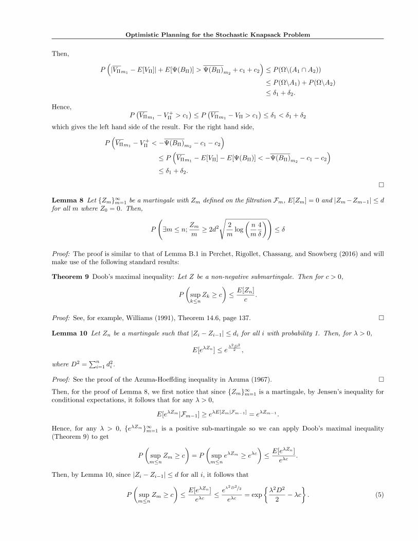
Lemma 8 Let Zm∞m=1 be a martingale with Zm defined on the filtration Fm, E[Zm] = 0 and |Zm−Zm−1| ≤ dfor all m where Z0 = 0. Then,

P

(∃m ≤ n;

Zmm≥ 2d2

√2

mlog

(n

m

4

δ

))≤ δ

Proof: The proof is similar to that of Lemma B.1 in Perchet, Rigollet, Chassang, and Snowberg (2016) and willmake use of the following standard results:

Theorem 9 Doob’s maximal inequality: Let Z be a non-negative submartingale. Then for c > 0,

P

(supk≤n

Zk ≥ c)≤ E[Zn]

c.

Proof: See, for example, Williams (1991), Theorem 14.6, page 137.

Lemma 10 Let Zn be a martingale such that |Zi − Zi−1| ≤ di for all i with probability 1. Then, for λ > 0,

E[eλZn ] ≤ eλ2D2

2 ,

where D2 =∑ni=1 d

2i .

Proof: See the proof of the Azuma-Hoeffding inequality in Azuma (1967).

Then, for the proof of Lemma 8, we first notice that since Zm∞m=1 is a martingale, by Jensen’s inequality forconditional expectations, it follows that for any λ > 0,

E[eλZm |Fm−1] ≥ eλE[Zm|Fm−1] = eλZm−1 .

Hence, for any λ > 0, eλZm∞m=1 is a positive sub-martingale so we can apply Doob’s maximal inequality(Theorem 9) to get

P

(supm≤n

Zm ≥ c)

= P

(supm≤n

eλZm ≥ eλc)≤ E[eλZn ]

eλc.

Then, by Lemma 10, since |Zi − Zi−1| ≤ d for all i, it follows that

P

(supm≤n

Zm ≥ c)≤ E[eλZn ]

eλc≤ eλ

2D2/2

eλc= exp

λ2D2

2− λc

. (5)


Minimizing the right hand side with respect to λ gives λ = cD2 and substituting this back into (5) gives,

P

(supm≤n

Zm ≥ c)≤ exp

− c2

2D2

.

Then, since we are considering the case where di = d for all i, D2 = nd2 and so,

P

(supm≤n

Zm ≥ c)≤ exp

− c2

2nd2

.

Further, if we are interested in P (supk≤m≤n Zm ≥ c), we can redefine the indices to get

P

(sup

k≤m≤nZm ≥ c

)= P

(sup

m′≤n−k+1Zm ≥ c

)≤ exp

− c2

2(n− k + 1)d2

. (6)

We then define εm = 2d√

1m log

(nm

8δ

)and use a peeling argument similar to that in Lemma B.1 of Perchet et al.

(2016) to get

P

(∃m ≤ n;

Zmm≥ εm

)≤blog2(n)c+1∑

t=0

P

2t+1−1⋃m=2t

Zmm≥ εm

(by union bound)

≤blog2(n)c+1∑

t=0

P

2t+1−1⋃m=2t

Zmm≥ ε2t+1

(since εm decreasing in m)

≤blog2(n)c+1∑

t=0

P

2t+1−1⋃m=2t

Zm ≥ 2tε2t+1

(as m ≥ 2t)

≤blog2(n)c+1∑

t=0

exp

− (2tε2t+1)2

2t+1d2

(from (6))

≤blog2(n)c+1∑

t=0

2t+1δ

8n(substituting ε2t+1)

≤ 2log2(n)+3δ

8n= δ. (since

k∑i=1

2i = 2k+1 − 1)

Proposition 11 (Proposition 2 in main text) The Algorithm BoundValueShare (Algorithm 2) returns confidencebounds,

L(V +Π ) = VΠm1

−

√Ψ(B)2 log(2/δ1)

2m1U(V +

Π ) = VΠm1+Ψ(BΠ)m2

+

√Ψ(B)2 log(2/δ1)

2m1+2Ψ(B)

√1

m2log

(8n

δ2m2

)which hold with probability 1− δ1 − δ2.

Proof: We begin by noting that our samples of item size are dependent since in each iteration we construct abound based on past samples and we use this bound to decide if we need to continue sampling or if we can stop.To model this dependence let us introduce a stopping time τ such that τ(ω) = n if our algorithm exits the loopat time n. Consider the sequence

Ψ(BΠ)1∧τ ,Ψ(BΠ)2∧τ , . . .

and define for m ≥ 1Mm = (m ∧ τ)(Ψ(BΠ)m∧τ − E[Ψ(BΠ)]) with M0 = 0.


Furthermore, define the filtration Fm = σ(BΠ,1, . . . , BΠ,m) then for m ≥ 1

E[Mm|Fm−1] = E[Mm|Fm−1, τ ≤ m− 1] + E[Mm|Fm−1, τ > m− 1].

NowE[Mm|Fm−1, τ ≤ m− 1] = E[Mm−1|τ ≤ m− 1].

and due to independence of the samples BΠ,1, . . . , BΠ,m

E[Mm|Fm−1, τ > m− 1]

= E[m(Ψ(BΠ)m − E[Ψ(BΠ)])|Fm−1, τ > m− 1]

= E

m−1∑j=1

Ψ(BΠ,j) + Ψ(BΠ,m)−mE[Ψ(BΠ)]

∣∣∣∣Fm−1, τ > m− 1

= (m− 1)E[Ψ(BΠ)m−1 − E[Ψ(BΠ)]|Fm−1, τ > m− 1]

+ E[Ψ(BΠ,m)− E[Ψ(BΠ)]|Fm−1, τ > m− 1]

= E[Mm−1|τ > m− 1] + E[Ψ(BΠ,m)]− E[Ψ(BΠ)] = E[Mm−1|τ > m− 1].

Hence, E[Mm|Fm−1] = Mm−1 and Mm is a martingale with increments |Mm−Mm−1| ≤ |Ψ(BΠ,m)−E[Ψ(BΠ)]| ≤Ψ(B). We could apply the Azuma-Hoeffding inequality to gain guarantees for individual m-values. Alternatively,we can use Lemma 8 to get,

P

(supm≤n

Mm

m≥ 2Ψ(B)

√1

mlog

(8n

δm

))≤ δ2.

Combining this with the argument in Lemma 1 gives

VΠm1− c1 ≤ V +


+ c1 + c2,

where c1 :=√

Ψ(B)2 log(2/δ1)2m1

and c2 := 2Ψ(B)

√1m2

log(

8nδ2m2

)and these bounds hold with probability 1−δ1−δ2.

Lemma 12 With probability 1 − δ0,1 − δ0,2, the bounds generated by BoundValueShare with parameters δ1,d =δ0,1d∗ N

−1d and δ2,d =

δ0,2d∗ N

−1d hold for all policies Π of depth d = d(Π) ≤ d∗ simultaneously.

Proof: The probability that all bounds hold simultaneously is P (⋂

Π∈PL(V +Π ) ≤ VΠ ≤ U(V +

Π )) where P is

the set of all policies. From Proposition 2, for any policy Π of depth d = d(Π), P (L(V +Π ) ≤ VΠ ≤ U(V +

Π )) ≥1− δd,1 − δd,2. Then,

P

( ⋂Π∈PL(V +

Π ) ≤ VΠ ≤ U(V +Π )

)= 1− P

( ⋃Π∈PL(V +

Π ) ≤ VΠ ≤ U(V +Π )c

)≥ 1−

∑Π∈P

P (L(V +Π ) ≤ VΠ ≤ U(V +

Π )c)

≥ 1−∑Π∈P

(δd(Π),1 + δd(Π),2)

= 1−d∗∑d=1

Nd(δd,1 + δd,2)

≥ 1−d∗∑d=1

Nd

(δ0,1d∗

N−1d +

δ0,2d∗

N−1d(Πt)

)

= 1−d∗∑d=1

1

d∗(δ0,1 + δ0,2) = 1− δ0,1 − δ0,2


D.2 Theoretical Results for Optimistic Stochastic Knapsacks (OpStoK)

Proposition 13 (Proposition 4 in main text) With probability at least (1 − δ0,1 − δ0,2), the algorithm OpStoK

returns a policy with value at least v∗ − ε.

Proof: The proof follows from the following lemma.

Lemma 14 For every round of the algorithm and incomplete policy Π, let D(Π) be the set of all descendants ofΠ. Define the event A =

⋂Π′∈D(Π)VΠ′ ∈ [L(V +

Π ), U(V +Π )]. Then P (A) ≥ 1− δ0,1 − δ0,2.

Proof: When BoundValueShare is called for a policy Π with d(Π) = d, it is done so with parameters δd,1 =δ0,1d∗ N

−1d and δd,2 =

δ0,2d∗ N

−1d , where δd,1 and δd,2 are used to control the accuracy of the estimated value of VΠ

and EΨ(BΠ) respectively. It follows from Proposition 2, that for any active policy Π, the probability that the

interval[VΠm1

− c1, VΠm1+ Ψ(BΠ)m2

+ c1 + c2

]generated by BoundValueShare does not contain V +

Π is less

than δd,1 + δd,2. Furthermore, from standard Hoeffding bounds, the probability that VΠ is outside the interval[VΠ − c1, VΠ + c1] is less than δd,1. Since any descendant policy Π′ of Π consists of adding at least one item tothe knapsack and item rewards are all ≥ 0, it follows that VΠ ≤ VΠ′ ≤ V +

Π . Hence, the probability of the valueof a descendant policy being outside the interval [L(V +

Π ), U(V +Π )] is less than δd,1 + δd,2. By the same argument

as in Lemma 12, it can be shown that P (A) > 1−∑d∗

d=1(δd,1 + δd,2)Nd = 1− δ0,1 − δ0,2.

The result of the proposition follows by noting that the true optimal policy ΠOPT will be a descendant of Πi

for some i ∈ I. Let Π∗ be the policy outputted by the algorithm. By the stopping criterion, L(V +Π∗) + ε ≥

maxΠ∈Active\Π∗ ≥ U(V +Π ) for any Π ∈ Active. From the expansion rule of OpStoK, it follows that either

ΠOPT ∈ Active or there exists some ancestor policy Π′ of ΠOPT in Active. In the first case, VΠOPT = v∗ ≤U(V +

ΠOPT) whereas in the latter VΠOPT = v∗ ≤ U(V +

Π′) with high probability from Lemma 14. In either case, it

follows that L(V +Π∗) + ε ≥ v∗ and so VΠ∗ + ε ≥ v∗.

Lemma 15 If Π is a complete policy then, U(V +Π )− L(V +

Π ) ≤ ε, otherwise U(V +Π )− L(V +

Π ) ≤ 6EΨ(BΠ)− 34ε.

Proof: By the bounds in Proposition 2, U(V +Π ) − L(V +

Π ) ≤ Ψ(BΠ)m2+ c2 + 2c1 = U(Ψ(BΠ)) + 2c1. For a

complete policy, U(Ψ(BΠ)) ≤ ε2 and according to BoundValueShare, m1 is chosen such that 2c1 ≤ ε

2 which

implies U(V +Π )− L(V +

Π ) ≤ ε.If Π is not complete, by the sampling strategy in BoundValueShare, we continue sampling the remaining budgetuntil L(Ψ(BΠ)) ≥ ε

4 . In this setting, the maximal width of the confidence interval of EΨ(BΠ) will satisfy

2c2 ≤ EΨ(BΠ)− ε

4. (7)

Hence,

U(V +Π )− L(V +

Π ) ≤ U(Ψ(BΠ)) + 2c1

≤ 3U(Ψ(BΠ)) (8)

≤ 3(EΨ(BΠ) + 2c2)

≤ 3(EΨ(BΠ) + EΨ(BΠ)− ε

4

)(9)

≤ 6EΨ(BΠ)− 3

4ε.

Where (8) follows since, when L(Ψ(BΠ)) ≥ ε4 , we sample the value of policy Π until c1 ≤ U(Ψ(BΠ)), and (9) by

substituting in (7).

Lemma 16 (Lemma 3 in main text) Assume that L(V +Π ) ≤ VΠ ≤ U(V +

Π ) holds simultaneously for all policiesΠ ∈ Active with U(V +

Π ) and L(V +Π ) as defined in Proposition 2. Then, Πt ∈ Qε for every policy selected by

OpStoK at every time point t, except for possibly the last one.


Proof: Since, when we expand a policy, we replace it in Active by all its child policies, at any time point t ≥ 1there will be one ancestor of Π∗ in the active set, denote this policy by Π∗t . If Πt = Π∗t , then by Lemma 14,VΠ∗ ∈ [L(V +

Πt), U(V +

Πt)]. Hence,

VΠ + 6EΨ(BΠ) +3

4ε ≥ U(V +

Π ) ≥ v∗ ≥ v∗ − 6EΨ(BΠ)− 3

4ε+ ε.

Where the last inequality will hold for any incomplete policy (since for an incomplete policy L(BΠ) ≥ ε4 ) and

so, Πt ∈ Qε. For Πt = Π∗, since 64ε ≥ ε, Πt ∈ Qε.

Assume Πt 6= Π∗t . If Πt is a complete policy, U(V +Πt

) − L(V +Πt

) ≤ ε. For a complete policy Π to be selected, it

must have the largest U(V +Π ), since most alternative policies will have larger U(Ψ(BΠ)). Hence Π

(1)t = Πt and

L(V +

Π(1)t

) + ε ≥ U(V +

Π(1)t

) ≥ maxΠ∈Active\Π(1)

t U(V +

Π ),

so the algorithm stops.

Assume Πt = Π(1)t 6= Π∗t is an incomplete policy. By Lemma 15, for an incomplete policy,

U(V +Π )− L(V +

Π ) ≤ 3U(Ψ(BΠ)) ≤ 6EΨ(BΠ)− 3

4ε. (10)

Then, if the termination criteria is not met,

VΠt ≥ L(V +Πt

) =⇒ VΠt + 6EΨ(BΠ)− 3

4ε− ε ≥ L(V +

Πt) + 6EΨ(BΠ)− 3

4ε− ε

≥ U(V +Πt

)− ε≥ max

Π∈Active\ΠtU(V +

Π )− ε

≥ L(V +Πt

)

≥ U(V +Πt

)− 6EΨ(BΠ) +3

4ε

≥ U(V +Π∗t

)− 6EΨ(BΠ) +3

4ε

≥ v∗ − 6EΨ(BΠ) +3

4ε

which follows since Π(1)t is chosen to be the policy with largest upper bound. Therefore, Πt ∈ Qε.

By the stopping criteria of OpStoK, if the algorithm does not stop and select Π(1)t as the optimal policy, then

Πt = Π(2)t and

L(V +

Π(1)t

) + ε < maxΠ∈Active\Π(1)

t U(V +

Π ) = U(V +

Π(2)t

).

By equation (10),

L(V +

Π(1)t

) + 6EΨ(BΠ)− 3

4ε ≥ U(V +

Π(1)t

).


and by the selection criterion U(Ψ(BΠ

(2)t

)) ≥ U(Ψ(BΠ

(1)t

)). Therefore, for Πt = Π(2)t 6= Π∗t ,

VΠt + 12EΨ(BΠ)− 6

4ε− ε ≥ L(V +

Πt) + 6EΨ(BΠt)−

3

4ε+ 6EΨ(BΠt)−

3

4ε− ε

≥ U(V +Πt

) + 6EΨ(BΠt)−3

4ε− ε

≥ U(V +Πt

) + 3U(Ψ(BΠt))− ε≥ U(V +

Πt) + 3U(Ψ(B

Π(1)t

))− ε

≥ L(V +

Π(1)t

) + 3U(Ψ(BΠ

(1)t

))

≥ U(V +

Π(1)t

)

≥ U(V +Π∗t

)

≥ v∗.

Hence Πt ∈ Qε.

Theorem 17 (Theorem 5 in main text) The total number of samples required by OpStoK is bounded from aboveby, ∑

Π∈Qε(m1(Π) +m2(Π)) d(Π),

with probability 1− δ0,2.

Proof: The result follows from the following three lemmas.

Lemma 18 For Π ∈ Aε of depth d = d(Π), then, with probability 1− δd,2, the minimum number of samples ofthe value and remaining budget of the policy Π are bounded by

m1(Π) =

⌈8Ψ(B)2 log( 2

δd,1)

ε2

⌉and m2(Π) = m∗,

where m∗ is the smallest integer satisfying 16Ψ(B)2

(EΨ(BΠ)−ε/2)2 ≤ mlog(8n/mδ2) with n defined as in (2).

Proof: When EΨ(BΠ) ≤ ε4 , the event U(Ψ(BΠ)) ≤ ε

2 will eventually occur with enough samples of theremaining budget of the policy. With probability greater than 1−δd,2, this will happen when 2c2 ≤ ε

2−EΨ(BΠ),

since by Hoeffding’s Inequality we know Ψ(BΠ)m2∈ [EΨ(BΠ) − c2, EΨ(BΠ) + c2] where c2 is as defined in

Lemma 1. From this, it follows that U(Ψ(BΠ)) ∈ [EΨ(BΠ), EΨ(BΠ) + 2c2]. We want to make sure thatU(Ψ(BΠ)) ≤ ε

2 will eventually happen so we need to construct a confidence interval such that c2 satisfiesEΨ(BΠ) + 2c2 ≤ ε

2 . Therefore we select m2 such that,

2c2 ≤ε

2− EΨ(BΠ)

=⇒ 4Ψ(B)

√2 log( 8n

m2δd,2)

m2≤ ε

2− EΨ(BΠ)

=⇒ 16Ψ(B)2

(EΨ(BΠ)− ε/2)2≤ m2

log(4n/m2δ2).

Defining, m2(Π) = m∗, where m∗ is the smallest integer satisfying the above, is therefore an upper bound onthe minimum number of samples necessary to ensure that U(Ψ(BΠ)) ≤ ε

2 with probability greater than 1− δd,2.

When U(Ψ(BΠ)) ≤ ε2 , BoundValueShare requires m1(Π) =

⌈2Ψ(B)2 log( 2

δd,1)

ε2

⌉samples of the value of the policy

to ensure 2c1 ≤ ε2 .


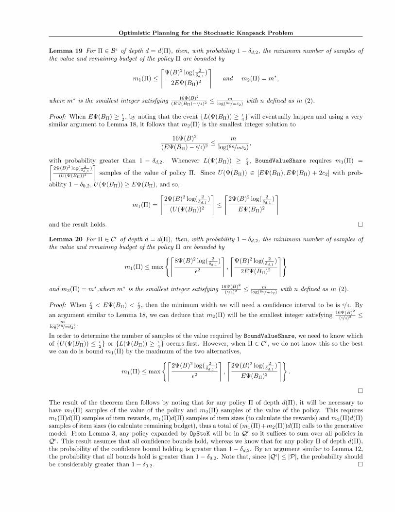
Lemma 19 For Π ∈ Bε of depth d = d(Π), then, with probability 1 − δd,2, the minimum number of samples ofthe value and remaining budget of the policy Π are bounded by

m1(Π) ≤

⌈Ψ(B)2 log( 2

δd,1)

2EΨ(BΠ)2

⌉and m2(Π) = m∗,

where m∗ is the smallest integer satisfying 16Ψ(B)2

(EΨ(BΠ)−ε/4)2 ≤ mlog(8n/mδ2) with n defined as in (2).

Proof: When EΨ(BΠ) ≥ ε2 , by noting that the event L(Ψ(BΠ)) ≥ ε

4 will eventually happen and using a verysimilar argument to Lemma 18, it follows that m2(Π) is the smallest integer solution to

16Ψ(B)2

(EΨ(BΠ)− ε/4)2≤ m

log(8n/mδ2),

with probability greater than 1 − δd,2. Whenever L(Ψ(BΠ)) ≥ ε4 , BoundValueShare requires m1(Π) =⌈

2Ψ(B)2 log( 2δd,1

)

(U(Ψ(BΠ))2

⌉samples of the value of policy Π. Since U(Ψ(BΠ)) ∈ [EΨ(BΠ), EΨ(BΠ) + 2c2] with prob-

ability 1− δ0,2, U(Ψ(BΠ)) ≥ EΨ(BΠ), and so,

m1(Π) =

⌈2Ψ(B)2 log( 2

δd,1)

(U(Ψ(BΠ))2

⌉≤

⌈2Ψ(B)2 log( 2

δd,1)

EΨ(BΠ)2

⌉

and the result holds.

Lemma 20 For Π ∈ Cε of depth d = d(Π), then, with probability 1 − δd,2, the minimum number of samples ofthe value and remaining budget of the policy Π are bounded by

m1(Π) ≤ max

⌈8Ψ(B)2 log( 2

δd,1)

ε2

⌉,

⌈Ψ(B)2 log( 2

δd,1)

2EΨ(BΠ)2

⌉

and m2(Π) = m∗,where m∗ is the smallest integer satisfying 16Ψ(B)2

(ε/4)2 ≤ mlog(8n/mδ2) with n defined as in (2).

Proof: When ε4 < EΨ(BΠ) < ε

2 , then the minimum width we will need a confidence interval to be is ε/4. By

an argument similar to Lemma 18, we can deduce that m2(Π) will be the smallest integer satisfying 16Ψ(B)2

(ε/4)2 ≤m

log(8n/mδ2) .

In order to determine the number of samples of the value required by BoundValueShare, we need to know whichof U(Ψ(BΠ)) ≤ ε

2 or L(Ψ(BΠ)) ≥ ε4 occurs first. However, when Π ∈ Cε, we do not know this so the best

we can do is bound m1(Π) by the maximum of the two alternatives,

m1(Π) ≤ max

⌈2Ψ(B)2 log( 2

δd,1)

ε2

⌉,

⌈2Ψ(B)2 log( 2

δd,1)

EΨ(BΠ)2

⌉.

The result of the theorem then follows by noting that for any policy Π of depth d(Π), it will be necessary tohave m1(Π) samples of the value of the policy and m2(Π) samples of the value of the policy. This requiresm1(Π)d(Π) samples of item rewards, m1(Π)d(Π) samples of item sizes (to calculate the rewards) and m2(Π)d(Π)samples of item sizes (to calculate remaining budget), thus a total of (m1(Π)+m2(Π))d(Π) calls to the generativemodel. From Lemma 3, any policy expanded by OpStoK will be in Qε so it suffices to sum over all policies inQε. This result assumes that all confidence bounds hold, whereas we know that for any policy Π of depth d(Π),the probability of the confidence bound holding is greater than 1− δd,2. By an argument similar to Lemma 12,the probability that all bounds hold is greater than 1− δ0,2. Note that, since |Qε| ≤ |P|, the probability shouldbe considerably greater than 1− δ0,2.

optimistic planning for the stochastic knapsack problem(2013) works with a knapsack size that...

Documents