Optimised KD-trees for fast image descriptor matching

Chanop Silpa-Anan Richard HartleySeeing Machines, Canberra Australian National University and NICTA.

Abstract

In this paper, we look at improving the KD-tree for a spe-cific usage: indexing a large number of SIFT and other typesof image descriptors. We have extended priority search, topriority search among multiple trees. By creating multipleKD-trees from the same data set and simultaneously search-ing among these trees, we have improved the KD-tree’ssearch performance significantly. We have also exploited thestructure in SIFT descriptors (or structure in any data set)to reduce the time spent in backtracking. By using Princi-pal Component Analysis to align the principal axes of thedata with the coordinate axes, we have further increasedthe KD-tree’s search performance.

1. Introduction

Nearest neighbour search is an important component inmany computer vision applications. In this paper, we lookat the specific problem of matching image descriptors for anapplication such as image retrieval or recognition. We de-scribe and analyze a search method based on using multiplerandomized KD-trees, and achieve look-up results signifi-cantly superior to the priority KD-trees suggested by Lowein [10] for this purpose. The randomized KD-tree approachdescribed here has been used recently in [15] for featurelookup for a very large image recognition problem.

The SIFT descriptor (Scale invariant feature) [11] is ofparticular interest because it performs well compared withother types of image descriptors in the same class [13]. ASIFT descriptor is a 128-dimensional vector normalised tolength one. It characterises a local image patch by captur-ing local gradients into a set of histograms which are thencompacted into one descriptor vector. In a typical applica-tion, a large number of SIFT descriptors extracted from oneor many images are stored in a database. A query usuallyinvolves finding the best matched descriptor vector(s) in thedatabase to a SIFT descriptor extracted from a query image.

A useful data-structure for finding nearest-neighbour

1This research was partly supported by NICTA, a research centrefunded by the Australian Government as represented by the Department ofBroadband, Communications and the Digital Economy and the AustralianResearch Council through the ICT Centre of Excellence program.

queries for image descriptors is the KD-tree [4], which isa form of balanced binary search tree.

Outline of KD-tree search. The general idea behindKD-trees is described now. The elements stored in theKD-tree are high-dimensional vectors in Rd. At the first level(root) of the tree, the data is split into two halves by a hyper-plane orthogonal to a chosen dimension at a threshold value.Generally, this split is made at median in the dimension withthe greatest variance in the data set. By comparing the queryvector with the partitioning value, it is easy to determine towhich half of the data the query vector belongs. Each of thetwo halves of the data is then recursively split in the sameway to create a fully balanced binary tree. At the bottom ofthe tree, each tree node corresponds to a single point in thedata set; though in some implementation, the leaf nodes maycontain more than one point. The height of the tree will belog2 N where N is the number of points in the data set.

Given a query vector, a descent down the tree requireslog2 N comparisons and leads to a single leaf node. The datapoint associated with this first node is the first candidate forthe nearest neighbour. It is useful to remark, that each nodein the tree corresponds to a cell in Rd, as shown in figure 1.And a search with a query point lying anywhere in a givenleaf cell will lead to the same leaf node.

The first candidate will not necessarily be the nearestneighbour to the query vector; it must be followed by aprocess of backtracking, or iterative search, in which othercells are searched for better candidates. The recommendedmethod is priority search [2, 4] in which the cells aresearched in the order of their distance from the query point.This may be accomplished efficiently using a priority treefor ordering the cells; see figure 1 in which the cells are num-bered in the order of their distance from the query vector.The search terminates when there are no more cells withinthe distance defined by the best point found so far. Note thatthe priority queue is a dynamic structure that is built whilethe tree is being searched.

In high dimensions to find the nearest neighbour may re-quire searching a very large number of nodes. This prob-lem may be overcome at the expense of an approximateanswer by terminating the search after a specified numberof nodes are searched (or earlier if the search terminates).

Figure 1. [Priority search of a KD-tree] In this figure, a querypoint is represented by the red dot and its closest neighbour liesin cell 3. A priority search first descends the tree and finds the cellthat contains the query point as the first candidate (label 1). How-ever, a point contained in this cell is often not the closest neigh-bour. A priority search proceeds in order through other nodes ofthe tree in order of their distance from the query point – that is,in this example through the nodes labelled 2 to 5. The search isbounded by a hypersphere of radius r (the distance between thequery point and the best candidate). The radius r is adjusted whena better candidate is found. When there are no more cells withinthis radius, the search terminates. KD-tree diagram thanks to P.Mondrian.

0

0.2

0.4

0.6

0.8

1

0 100 200 300 400 500 600 700 800 900 1000

p(e

rror

)

Maximum number of searched nodes

KD-tree’s error

priority searchstandard search

Figure 2. [Search performance] When a search is restricted tosome maximum number of searched nodes, the probability of find-ing the true nearest neighbour increases with the increasing limit.Priority search increases search performance, compared with atree backtracking search.

This graph and subsequence graphs are made by searchingSIFT descriptors from a data set of size approximately 500 000points. A query is a descriptor drawn from the data set and cor-rupted with Gaussian noise. A nearest neighbour query result iscompared with the true nearest match.

00.20.40.60.8

11.21.4

0 100 200 300 400 500 600 700 800 900 1000

−lo

gp(e

rror

)

Maximum number of searched nodes

Negative log of KD-tree’s error

priority searchwish

Figure 3. [Diminished returns] This figure is essentially the sameas figure 2 (lower curve), but on a negative logarithmic scale.Suppose each search of m nodes is independent and has a fail-ure probability pe. By searching n nodes the error rate reduces tope

n/m. On a logarithmic scale, this is a straight line with a slopeof (n/m) log pe. The figure shows that increasing the number ofsearched nodes for KD-tree does not lead to independent searches,and gives diminished returns.

The best candidate may be the exact nearst neighbour withsome acceptable probability that increases as more nodesare searched (see figure 2).

Unfortunately, extending the search to more and morenodes leads to diminishing returns, in which we have towork harder and harder to increase the probability of find-ing the nearest neighbour. This point is illustrated in fig-ure 3. The main purpose of this paper is to propose methodsof avoiding this problem of diminishing returns by carryingout simultaneous independent searches in different trees.

The problem with diminishing returns in priority searchis that searches of the individual nodes in a tree are not inde-pendent, and the more searched nodes, the further away thenodes are from the node that contain the query point. To ad-dress this problem, we investigate the following strategies.

1. We create m different KD-trees each with a differentstructure in such a way that searches in the differenttrees will be (largely) independent.

2. With a limit of n nodes to be searched, we break thesearch into simultaneous searches among all the mtrees. On the average, n/m nodes will be searched ineach of the trees.

3. We use Principal Component Analysis (PCA) to rotatethe data to align its moment axes with the coordinateaxes. Data will then be split up in the tree by hyper-planes perpendicular to the principal axes.

By either using multiple search-trees or by building theKD-tree from data realigned according to its principal axes,search performance improves and even improves furtherwhen both techniques are used together.

Previous work

The KD-tree was introduced in [5] as a generalisation of abinary tree to high dimensions. Several variations in buildinga tree, including randomisation in selecting the partitioningvalue, were suggested. Later on, an optimised KD-tree with atheoretic logarithmic search-time was proposed in [7]. How-ever, this logarithmic search-time does not apply to trees ofhigh dimension, where the search time may become almostlinear.

Thus, although KD-trees are effective and efficientin low dimensions, their efficiency diminishes for high-dimensional data. This is because with high dimensionaldata, a KD-tree usually takes a lot of time to backtrackthrough the tree to find the optimal solution. By limiting theamount of backtracking, the certainty of finding the absoluteminimum is sacrificed and replaced with a probabilistic per-formance. Recent research has therefore aimed at increas-ing the probability of success while keeping backtrackingwithin reasonable limits. Two similar approximated searchmethods, a best-bin-first search and a priority search wereproposed in [2, 4], and these methods have been used withsignificant success in object recognition ([10]).

In the vision community, interest in large scale nearest-neighbour search has increased recently, because of its evi-dent importance in object recognition as a means of lookingup feature points, such as SIFT features in a database. No-table work in this area has been [14, 15]. It was reported in[15] that KD-trees gave better performance than Nister’s vo-cabulary trees [14] as an aid to K-means clustering. In thispaper therefore we concentrate on methods of improvingthe performance of KD-trees, and demonstrating significantimprovements in this technique.

Our KD-tree method is related to randomized trees, asused in [9], based on earlier work in [1]. However, our meth-ods are not directly comparable with theirs, since we ad-dress different problems. Randomized trees are used in [9]for direct recognition, whereas we are concerned with themore geometric problem of nearest-neighbour search. Sim-ilarly, more recent work of Grauman [8] uses random hash-ing techniques for matching sets of features, but their algo-rithm is not directly comparable with ours. Finally, locality-sensitive hashing (LSH) [6] is based on similar techniquesas ours, namely projection of the data in different random di-rections. Whereas LSH projects the data onto different lines,in our case we consider randomly reorienting the data, whichis related to projection onto differently oriented linear sub-spaces. Like KD-trees, LSHs also have trouble dealing withvery high dimensional data, and have not been used exten-sively in computer vision applications.

2. Independent multiple searches

When examining priority search results in a linear or alogarithmic scale (figure 2 and 3), it is clear that increas-ing the number of searched nodes increases the probabilityof finding the true nearest neighbour. Any newly examinedcell, however, depends on previously examined cells. Sup-pose each search is independentwith a failure probability p e.Searching independently n times reduces the failure proba-bility to pn

e . This is a straight line on a logarithmic scale. Itis clear that searches of successive nodes of the tree are notindependent, and searches of more and more nodes becomeless and less productive.

On the other hand, if KD-trees are built with differentparameters, with different ways to select partitioning valuefor example, the order of search node and search results onthese KD-trees may be different. This leads to the idea ofusing multiple search-trees to enhance independence.

Rotating the tree. Our method of doing independentmultiple searches is to create multiple KD-trees with dif-ferent orientations. Suppose we have a data set X = {x i}.Creating KD-trees with different orientations simply meanscreating KD-trees from rotated data Rxi, where R is a rota-tion matrix. A principal (a regular) KD-tree is one createdwithout any rotation, R = I. By rotating the data set, the re-sulting KD-tree has a different structure and covers a differ-ent set of dimensions compared with the principal tree. Analgorithm for searching on a rotated KD-tree is essentiallysearching a rotated tree with a rotated query point Rq.

Once a rotated tree is built, the rotated data set can bediscarded because all the information is kept inside the treeand the rotation matrix. Only the original vector is needed inorder to compute the distance between a point in the data setand a query. Under a rotation, the original distance ‖q − x i‖is the same as the rotated distance ‖Rq − Rxi‖.

Are rotated trees independent? To test whether searchesof differently rotated trees were independent, we carried outsuccessive searches over the same data set successively onmultiple trees. First, we searched the 20 closest nodes inone tree, then the closest 20 on the next tree, and so on, toa total of 200 nodes searched. The total cumulative (empir-ical) probability of failure was computed and plotted on anegative logarithmic scale. If the searches on different treeswere independent, this would give a linear graph. The re-sults are shown in figure 4, and support the hypothesis thatthe searches are independent. This test was done with ran-domly generated vectors. Tests done also with real SIFT fea-tures showed major improvements of using multiple searchtrees, compared with a single tree, as reported in figure 6.However in that case the hypothesis of independent searcheswas not quite so strongly sustained. Nevertheless, using mul-tiple trees goes a long way towards enabling independent

0

0.2

0.4

0.6

0.8

1

1.2

0 10 20 30 40 50 60 70 80 90

−lo

gp(e

rror

)

Maximum number of searched nodes

Negative log of KD-tree’s and NKD-tree’s error – synthetic data

KD-treeNKD-tree

Figure 4. [Independence of searches] This graph shows the re-sult of successive independent searches of 20 nodes on each of 9trees, showing the (empirical) negative log-likelihood of error. Ifthe searches on individual trees are independent, then this will bea straight-line through the origin. Visibly, the graph is approxi-mately linear, which supports a hypothesis of independence. Forcomparison we show the results for a single KD-tree as well.

searches, even if they are not completely independent.

A saving using Householder matrices. Computation ofRx in d dimensions has complexity O(d2). The underlyingidea of using a rotation matrix is to transform the data setonto different bases while preserving the norm. Almost anyorthogonal transformationmatrix can achieve this. A House-holder matrix of the form Hv = I − 2vv�/v�v is an or-thonormal transformation; it is a reflection through a planewith normal vector v. Multiplication of a vector and Hv canbe arranged such that it has complexity of O(d) instead ofO(d2). With the Householder transformation, m trees canbe built in O(mdN log N) time.

Searching multiple trees. With multiple trees, we need toexpand the concept of a priority search on a single tree. Con-ceptually, searching m trees with a limitation of n searchnodes is simply searching each tree for n/m nodes. This canbe easily implemented by searching trees sequentially. How-ever, this is not optimal, and besides does not scale to a casewhere we impose no limitation on the number of searchednodes (searching for the true nearest neighbour) because wewould already find the best solution and would not be re-quired to search extra trees.

We prefer to search multiple trees in the form of a concur-rent search with a pooled priority queue. After descendingeach of the trees to find an initial nearest-neighbour candi-date, we select the best one from all the trees. We then poolthe node ranking by using one queue to order the nodes fromall m trees. In this way, nodes are not only ranked againstother nodes within the same tree, but also ranked againstother nodes in all trees. As a result, nodes from all the trees

are searched in the order of their distance from the querypoint simultaneously.

With these modifications, we use the term NKD-tree fora data structure of multiple KD-trees with different orienta-tions.

Space requirements. For large data sets it is important toconsider the space requirements for holding large numbersof trees. We have implemented our KD-trees as pointerlesstrees, in which the nodes are kept in a linear array. The twochildren of node n are the nodes at positions 2n and 2n + 1in the array. Only the number of the splitting dimension (onebyte) and the splitting value (one byte for SIFT descriptorscontaining single byte data, or 4 bytes for floating point data)need to be stored at internal nodes in the tree. The leaf nodesmust contain an index to the associated point. In total thismeans 6N bytes for a tree with N elements. In addition, theactual data vectors must be stored, but only once. Thus, withone million data vectors of dimension 128, the storage re-quirement is 128MB for the data vectors (or 512MB if floatdata is used), and for each independent tree only 6MB. Thus,the storage overhead for having multiple trees is minimal.

A different randomisation: RKD-tree. The purpose ofthe rotation is to create KD-trees with different structures.Instead of explicitly rotating the tree, using randomness onparameters can also alter the tree structure. In fact, the parti-tioning value was originally selected randomly [5] while thepartitioning dimension was selected in cyclical order. Thisapproach was later on abandoned in an optimal KD-tree [7]and in other splitting rules [3].

In accordance with the principle of selecting a partition-ing value in the dimension with the greatest variance, weconsidered creating extra search trees with the followingidea. In the standard KD-tree, the dimension which the datais divided is the one in which the data has the greatest vari-ance. In reality, data variance is quite similar in many of thedimensions, and it does not make a lot of difference in whichof these dimensions the subdivision is made. We adopt thestrategy of selecting at random (at each level of the tree)the dimension in which to subdivide the data. The choice ismade from among a few dimensions in which the data hashigh variance. Multiple trees are constructed in this way, dif-ferent from each other in the choice of subdivision dimen-sions. By using this method, we retain high probability thata query can be on either half of the node, and at the sametime maintain backtracking efficiency.

In this randomisation strategy, in contrast to rotating thedata explicitly, the data set stays in the original space, thus,saving some computation on data projection while buildingthe tree. In searching SIFT descriptors, this randomised tree(RKD-tree) performs as well as NKD-tree. Also note that theRKD-tree has the same complexity level in storage as theNKD-tree.

3. Modelling KD-trees.

The following argument is meant to give an intuitive ideaof why using differently rotated trees will be effective. It isdifficult to model the performance of a KD-tree mathemat-ically, because of the the complexity of the priority searchprocess. In this section, it will be argued that the perfor-mance of a KD-tree is well modelled by projecting the datainto a lower dimensional space followed by testing the datain the order of its distance from a projected query point. Itwill be seen that modelling a KD-tree’s performance in thisway gives rise to performance graphs that strongly resemblethe actual performance of KD-trees on SIFT data.

Consider a KD-tree in a high-dimensional space, such asdimension 128 for SIFT features. If the tree contains onemillion nodes, then it has height 20. During a search with aquery point in the tree, no more than 20 of the of the entriesof the vector are considered. The other 108 entries are irrel-evant for the purposes of determining which cell the searchends up in. If q is the query vector and x is the vector asso-ciated with the leaf cell that the query vector leads to, thenq and x are close in 20 of their entries, but maybe no others.

The virtual projection. Typically only a small number nof the data dimensions will be used to partition the tree. Theother 128 − n dimensions will be unused, and irrelevant.Exactly the same tree will be obtained if the data is firstprojected by a projection π onto a subspace of dimensionn before building the tree. The subspace is aligned with thecoordinate axes. Since no actual projection takes place, werefer to this as a virtual projection – but since such a projec-tion would make no difference to the method of searchingthe KD-tree we may assume that this projection takes place,and the tree is built using the projected data.

Under priority search in the KD-tree, leaf nodes in the treeare searched in the order of the distance of the correspond-ing cells from the projected query point π(q). The points as-sociated with the cells are tested in that order to find the onethat is closest to q. Since the structure of the KD-tree maybe complex, we simplify the analysis by make a simplifyingassumption that searching the cells in this order is the sameas testing the points xi in the order of the distance of theirprojection π(xi) from the projected query point π(q). Sincethe tree is virtually built from the projected data, this is thebest search outcome that can be achieved. Thus it providesa best-possible performance for search in the KD-tree.

To summarise this discussion: in our model, the order inwhich points xi are tested to find the closest match to q isthe order of the distance of π(xi) from π(q) where π is aprojection onto a lower dimensional space.

Probability analysis. We have argued that KD-tree searchin high dimensions is closely related to nearest-neighboursearch after projection into a lower dimensional space. The

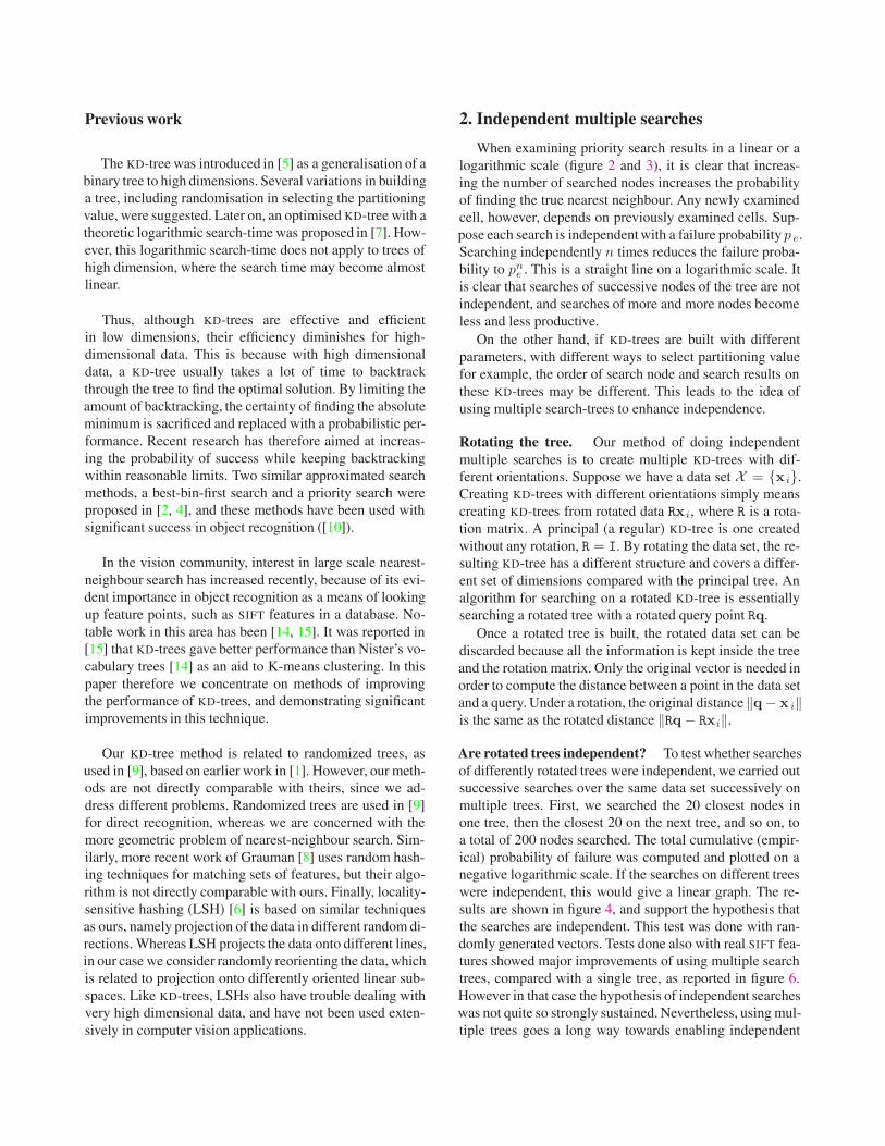
essential question here is whether the nearest neighbour toa query point in the high dimension will remain an approx-imate nearest neighbour after projection. Consider a largenumber of points x in a high-dimensional space, suppose qis a query point and xbest is the closest point to it. Now, letall points be projected to a lower dimensional space by a pro-jection π, and denote by p(n) the probability that π(xbest) isthe n-th closest point to π(q). We would expect that the mostlikely outcome is that π(xbest) is in fact the closest pointto π(q), but this is not certain. In fact, it does not happenwith high probability, as will be seen. It may be possible tocompute this probability directly under some assumptions.However, instead we computed the form of this probabilitydistribution empirically; the resulting probability distribu-tion function is shown in figure 5. The most notable featureis that this distribution has a very long tail. Also shown isthe cumulative probability of failure after testing m nodes,given by f(m) = 1 −

∑mi=1 p(i).

The simulation of figure 5 shows that the nearest-neighbour point to the query may be a very long way downthe list of best of closest matches when projected to low di-mension. Consequently the probability of failure f(m) re-mains relatively high even for large m. This indicates whysearching the list of closest neighbours in the KD-tree mayrequire a very large number of cells to be searched beforethe minimum is found.

On the other hand, the strategy of using several indepen-dent projections may give better results. If the data is rotated,then the virtual projection to a new n-dimensional subspacewill be in a different direction aligned with the new coordi-nate axes. If q and x are close to each other in the full space,then they will remain close under any projection, and hencewill belong to the same or neighbouring leaf cells in anyof the rotated KD-trees. On the other hand, points that arenot close may belong to neighbouring leaf cells under oneprojection, but are unlikely to be close under a different pro-jection. We model the probability of failure using k trees asthe product of the independent probabilities of failure fromsearching approximately m/k cells in each of the k trees.More exactly, if a = mmodk and mi = (m − a)/k, thenthe probability of failure when searching m i cells in k − atrees and mi + 1 cells in a trees (a total of m cells in all) isfm,k = f(mi)k−a f(mi + 1)a. The graphs of these prob-abilities are shown in figure 5 for several different valuesof k. They clearly show the advantage of searching in sev-eral independent projections. Using independent projectionsinto lower dimensional spaces boosts the probability thatthe closest point will be among the closest points in at leastone of the projections. The results obtained from this modelagree quite closely in form with the results obtained usingindependent KD-trees. This supports our thesis that closestpoint search in high dimensional KD-trees is closely relatedto nearest neighbour search in a low dimensional projection,

and that the long tail of the probability distribution p(n) isa major reason why searching in a single KD-tree will fail,whereas using several KD-trees with independently rotateddata will work much better.

Figure 5. Top left: Distribution of rank of best fit after projec-tion to low dimensions. 100, 000 random points in a hypercube inR128 are projected by a projection π into R20. The nearest pointxbest to a query q in R128 may become n-th closest after projec-tion onto R20. The x-axis is the ranking n and the y-axis shows theprobability that the projection π(xbest) will be n-th closest pointto π(q) in R20. The graph shows that the most likely ranking isfirst, but the graph has a long tail.Top right: Top line shows the cumulative failure rate. It rep-resents the probability of failure to find the best fit in R128

by examining the n best fits in R20. . Subsequent graphs showthe probability of finding the best fit by examining the clos-est n fits in m different independent projections for m =2, 3, 4, 5, 10, 20, 50, 100, 200, 1000. As may be seen, the more in-dependent projections are used, the better the chance of findingthe best fit xbest in R128 among the n points tested.Bottom left: Negative log likelihood of cumulative failure ratefor the same number of projections as above. If each independentquery (point tested) has independent probability of being the opti-mum point xbest, the lines will be straight. Bottom right: Closeup of the previous graph showing curvature of the graphs, andhence diminished returns from examining more and more pro-jected points.

4. Principal Component Trees

It has been suggested in the discussion of section 3 thatone of the main reasons that KD-trees perform badly in highdimensions is that points far from the query point q maybe projected (via a virtual projection) to points close to the

best match xbest. It makes sense therefore to minimize thiseffect to project the data in its narrowest direction. Sincein a KD-tree the data is divided up in the directions of thecoordinate axes, it makes sense to align these axes with theprincipal axes of the data set. Aligining data with principalaxes has been considered previously in, for instance [12].We show in this section that by combining this idea with theKD-tree data structure gives even better results.

To be precise, let {xi|i = 1, . . . , N} be a set of points inRd. We begin by translating the data set so that its centroid isat the origin. This being done, we now let A =

∑Ni=1 xixi

�.The eigenvectors of A are the principal axes of the data set,and the eigenvalues are referred to as the principal moments.If A = UΛU� is the eigenvalue decomposition of A, such thatthe columns of U are the (orthogonal) eigenvectors, then themapping xi �→ U�xi maps the points onto a set for whichthe principal axes are aligned with the coordinate axes. Fur-thermore, if U1:k is the matrix consisting of the k dominanteigenvectors, then U1:k

� projects the point set into the spacespanned by the k principal axes of the data.

Generally speaking if the data is aligned via the rota-tion U�, the dimensions along which data is divided in theKD-tree will be chosen from among the k principal axes ofthe data, where k is the depth of the tree (though this willnot hold strictly, especially near the leaves of the tree). Theeffect will be the same as if the data were projected via theprojection U1:k

� and the projected data were used to buildthe tree. In a sense the data is thinnest in the directions of thesmallest principal axes, and projection onto the space of thek dominant axes will involve the smallest possible change inthe data, and will minimize the possibility of distant pointsprojecting to points closer to xbest than π(q).

We therefore suggest the following modifications to theKD-tree algorithm.

1. Before building the tree, the data points x i should berotated via the mapping U� to align the principal axeswith the coordinate axes.

2. When using multiple trees, the rotation of the datashould be chosen to preserve the subspace spanned bythe k largest principal axes.

The resulting version of the KD-tree algorithm will be calledthe PKD-tree algorithm. The second conditions is reason-able, since it makes no sense to rotate the data to align itwith the coordinate axes and then unalign it using randomrotations while creating multiple trees.

Almost equivalent is to project the data to a lower dimen-sional subspace using the PCA projection U1:k

�, and thenuse this projected data to build multiple trees. (The only dif-ference is that in this way, the splitting dimension is strictlyconstrained to the top k principal axis directions.) An im-portant point which we emphasize is that the original unpro-jected data must still be used in testing the distance betweenthe query point q and candidate closest neighbours. The ef-

0

0.1

0.2

0.3

0.4

0.5

0.6

100 200 300 400 500 600 700 800 900 1000

p(e

rror

)

Maximum number of searched nodes

NKD-tree’s error

Figure 6. [An NKD-tree] This figure shows some search resultsusing an NKD-tree. From the top-most graph to the bottom-most graph are NKD-trees using from 1 to 6 search trees. TheNKD-tree’s performance increases with the increasing number ofsearched nodes and the increasing number of trees.

0

0.1

0.2

0.3

0.4

0.5

0.6

100 200 300 400 500 600 700 800 900 1000

p(e

rror

)

Maximum number of searched nodes

RKD-tree’s error

Figure 7. [An RKD-tree] In a similar setting to that of figure 6,the RKD-tree performs as well as the NKD-tree in searching SIFT

descriptors.

fect of projecting the data is only to constrain and guide thestructure and alignment of the KD-trees. The projected datais discarded once the tree is built.

5. Experimental results

For comparison, we use a data set of approximately500 000 SIFT descriptors, computed from 600 images. Ofthese descriptors, 20 000 descriptors are randomly pickedfor nearest neighbour queries; however, they are corruptedwith some small Gaussian noise with standard deviation0.05 in all 128 dimensions. Note that SIFT descriptors arenormalised to length 1 including ones used for queries;therefore the expected norm of the distance from the originalto the corrupted point is 0.5.

Figure 6 shows search results with an NKD-tree. Thenumber of search trees ranges from one to six trees; the lim-

0

0.1

0.2

0.3

0.4

0.5

0.6

100 200 300 400 500 600 700 800 900 1000

p(e

rror

)

Maximum number of searched nodes

PKD-tree’s error (128 dimensions)

Figure 8. [Multiple PKD-tree trees with unconstrained rotation]The PKD-tree with full 128 dimensions performs better than bothNKD-tree and RKD-tree. There is a significant improvement overa KD-tree when a single search tree is used. For multiple searchtrees, we allow the rotations of the data to be arbitrary. The per-formance continues to improve but is not so marked, because therotation of the data undoes the PCA alignment.

0

0.1

0.2

0.3

0.4

0.5

0.6

100 200 300 400 500 600 700 800 900 1000

p(e

rror

)

Maximum number of searched nodes

PKD-tree’s error (30 dimensions)

Figure 9. [A PKD-tree created with 30 dimensions] ThePKD-tree’s performance is at its best when rotations are con-strained to the optimal number of dimensions. This figure showsthe PKD-tree’s results when the data is projected by a projectionU1:k using PCAonto 30 dimensions. This constrains the rotationsused to build multiple trees so that they preserve the space spannedby the k = 30 principal axes. There are significant improvementscompared with the results shown in figure 8.

itation of searched nodes ranges from 100 to 1000 nodes.Clearly, the error reduces when we search more nodes. Atthe same number of search nodes, using more search treesalso reduces the error. In a similar setting, an RKD-tree per-forms as well as an NKD-tree; figure 7 shows these results.

For a PKD-tree, figure 8 shows results when the data isaligned using PCA, but multiple search trees are built withunconstrained rotations. In a single search tree case, there isa significant improvement over an ordinary KD-tree (com-pare the top most lines between figure 6 and figure 8). The

PKD-tree still performs better with an increasing number oftrees, however with a smaller increment.

We next explored the strategy of aligning the data usingPCA and then building multiple trees using rotations that fix(not pointwise) the space spanned by the top k = 30 prin-cipal axes. Our experiments showed that 30 is the optimalnumber for this purpose. In figure 9, we simply project thedata onto a subspace of dimension 30 using PCA, and thenallow arbitrary rotations of this projected data. It is a clearthat using multiple search trees with the trees built from anoptimal number of dimensions improves the result. There isa significant difference when six search trees are used.

This form of PKD-tree with multiple search trees givesa very substantial improvement over the standard singleKD-tree. By comparing the top line of figure 6 (single stan-dard KD-tree) with the bottom line of figure 9 (PKD-tree with6 trees), we see that the same search success rate achievedin 1000 nodes with the standard tree is reached in about150 nodes by the PKD-tree. Looked at a different way, aftersearching 1000 nodes, the standard KD-tree has about 75%success rate, whereas the multiple PKD-tree has over 95%success.

6. Conclusions

In the context of nearest neighbour query in a high di-mensional space with a structured data set – SIFT descrip-tors in 128 dimensions in our application – we have demon-strated that various randomisation techniques give enormousimprovements to the performance of the KD-tree algorithm.

The basic technique of randomisation is to carry outsimultaneous searches using several trees, each one con-structed using a randomly rotated (or more precisely, re-flected) data set. This technique can lead to an improvementfrom about 75% to 88% in successful search rate, or a 3-times search speed-up with the same performance.

Best results are obtained by combining this techniquewith a rotation of the data set to align it with its principalaxis directions using PCA, and then applying random House-holder transformations that preserve the PCA subspace of ap-propriate dimension (d′ = 30 in our trials). This leads to asuccess rate in excess of 95%.

Tests with synthetic high-dimensional data (not reportedin detail here) led to even more dramatic improvements, withup to 7-times diminished error rate with the NKD-tree algo-rithm alone.

References

[1] Y. Amit and D. Geman. Shape quantization and recognitionwith randomized trees. Neural Quantization, 9(7):1545 –1588, 1997. 3

[2] S. Arya and D. M. Mount. Algorithms for fast vector quan-

tization. In Proceedings of the data compression conference,pages 381 – 390, 1993. 1, 3

[3] Sunil Arya, David M. Mount, Nathan S. Netanyahu, RuthSilverman, and Angela Y. Wu. An optimal algorithm forapproximate nearest neighbor searching in fixed dimensions.Journal of the ACM, 45(6):891–923, 1998. 4

[4] Jeffrey S. Beis and David G. Lowe. Shape indexing usingapproximate nearest–neighbour search in high–dimensionalspaces. In Proceedings of computer vision and pattern recog-nition, pages 1000–1006, Puerto Rico, June 1997. 1, 3

[5] Jon Louis Bentley. Multidimensional binary search treesused for associative searching. Communications of the ACM,18(9):509–517, 1975. 3, 4

[6] M. Datar, N. Immorlica, P. Indyk, and V. Mirrokni. Locality-sensitive hashing scheme based on p-stable distributions. InProceedings of the symposium on computational geometry,pages 253–262, 2004. 3

[7] Jerome H. Freidman, Jon Louis Bently, and Raphael Ar-ifinkel. An algorithm for finding best matches in logarithmicexpected time. ACM transactions on mathematical software,3(3):209–206, september 1977. 3, 4

[8] K. Grauman and T. Darrell. Pyramid match hashing: Sub-linear time indexing over partial correspondences. In Proc.IEEE Conference on Computer Vision and Pattern Recogni-tion, 2007. 3

[9] V. Lepetit and P. Fua. Keypoint recognition using random-ized trees. IEEE Transactions on Pattern Analysis and Ma-chine Intelligence, 28(9):1465–1479, 2006. 3

[10] D. Lowe. Distinctive image features from scale invariantkeypoints. IJCV, 60(2):91 – 110, 2004. 1, 3

[11] David G. Lowe. Distictive image features from scale-invariant keypoints. International journal of computer vi-sion, 60(2):91–110, 2004. 1

[12] J. McNames. A fast nearest-neighbor algorithm based ona principal axis search tree. IEEE Transactions on PatternAnalysis and Machine Intelligence, 23:964–976, September201. 6

[13] Krystian Mikolajczyk and Cordelia Schmid. A performanceevaluation of local descriptors. In Proceedings of computervision and pattern recognition, 2003. 1

[14] D. Nister and H. Stewenius. Scalable recognition with a vo-cabulary tree. In Proc. IEEE Conference on Computer Vi-sion and Pattern Recognition, volume 2, pages 2161 – 2168,2006. 3

[15] J. Philbin, O. Chum, M. Isard, J. Sivic, and A. Zisser-man. Object retrieval with large vocabularies and fast spatialmatching. In Proc. IEEE Conference on Computer Visionand Pattern Recognition, 2007. 1, 3