Electronic copy available at: http://ssrn.com/abstract=1883519

Optimal Insurance Design

under Rank Dependent Utility

Carole Bernard∗, Xue Dong He†, Jia-An Yan‡ and Xun Yu Zhou§

July 10, 2011

Abstract

We derive explicitly the optimal insurance contract for an individual behaving

according to rank dependent utility as described in Quiggin (1993). The utility func-

tion is assumed to be concave and the probability distortion is reversed S-shaped.

We apply the technique of quantile formulation to solve this problem thoroughly,

and we show that the optimal contract fully insures small losses, and insures large

losses above a deductible. We finally compare, both analytically and numerically,

our result with those of models having convex or concave distortions.

Keywords : Optimal Insurance Design, Rank Dependent Utility, Behavioral Finance,

Decision making.

JEL Classification: G22, D81, D82.

∗c3bernar@uwaterloo.ca, University of Waterloo. C. Bernard acknowledges support from the Natu-ral Sciences and Engineering Research Council of Canada.

†Corresponding author. xh2140@columbia.edu, Department of IEOR, Columbia University, 316Mudd Building, 500 W. 120th Street, New York, NY 10027. X. D. He acknowledges the support from astart-up fund in Columbia University.

‡jayan@amt.ac.cn. Chinese Academy of Science, China. J.-A. Yan acknowledges supports from theNational Basic Research Program of China (973 Program) (No. 2007CB814902), the Key Laboratory ofRandom Complex Structures and Data Science, CAS (No. 2008DP173182), and the Science Fund forCreative Research Groups of NNSF (No. 11021161).

§zhouxy@maths.ox.ac.uk, Mathematical Institute, University of Oxford, 24-29 St Giles’, Oxford OX13LB, UK, and Department of Systems Engineering & Engineering Management, The Chinese Universityof Hong Kong, Shatin, Hong Kong. X. Y. Zhou acknowledges the support from a start-up fund of Oxford,as well as from the Nomura Centre and OMI.

1

Electronic copy available at: http://ssrn.com/abstract=1883519

1 Introduction

The classical theory of optimal insurance design takes place in the expected utility

(EU) framework and considers a risk-averse individual (see for example Arrow, 1963,

1971, Gollier, 1996, Gollier and Schlesinger, 1996, Raviv, 1979). Many extensions have

been investigated: one may change the premium principle (mean–variance principles have

been studied by Kaluska, 2001 and general premium principles can be found in Gajek

and Zagrodny, 2004), add a regulatory or solvency constraint (Bernard and Tian, 2009,

2010), assume that the insurer has limited liability (Cummins and Mahul, 2004), or relax

the non-negativity constraint on the indemnity (Gollier, 1987). One may also extend the

optimal insurance theory to non-expected utility frameworks, for example using Yaari’s

“dual theory of choice” (Doherty and Eeckhoudt, 1995).

The contribution of this paper is to extend the classical optimal insurance theory to

the case in which the insured’s preference is represented by Quiggin’s rank dependent

utility (RDU). Compared to EU, RDU captures individuals’ tendency of overweighting

small probabilities of both extremely good outcomes and bad ones, through a reversed S-

shaped probability distortion (or weighting) function. We find that the optimal insurance

contract in the framework of RDU (with a reversed S-shaped distortion function) is in

general not a deductible one, contrast to that in the framework of EU. Instead, the

optimal contract fully insures small losses, and insures large losses above a deductible. As

it has been widely acknowledged RDU is a more plausible representation of individuals’

preferences than EU, our results may lead to rethinking the optimal insurance contract

design.

There has already been a number of papers studying the optimal insurance problem

in the framework of RDU. Chateauneuf, Dana, and Tallon (2000) work in the Choquet

expected utility framework and give some results in the RDU framework as a special case.

2

Dana and Scarsini (2007) consider optimal risk sharing with background risk and briefly

discuss the case of RDU. Carlier and Dana (2005b) discuss the Pareto efficient insurance

contracts under RDU. However, all these three papers assume the individuals are strongly

risk averse1, which is represented by convex distortion functions in RDU. Similarly, Sung,

Yam, Yung, and Zhou (2011) find the optimal insurance contract when the distortion is

convex, although the utility function there is S-shaped as in cumulative prospect theory

(CPT) of Tversky and Kahneman (1992). Dana and Shahidi (2000) weaken the strong

risk aversion assumption to the left monotone risk aversion. However, this assumption still

contradicts the typical reversed S-shaped distortion function observed and calibrated from

actual human behavior2. Although Carlier and Dana (2008) consider two-persons efficient

risk-sharing problems for concave law-invariant utilities, which is again inconsistent with

RDU with reversed S-shaped distortion functions, they do give a characterization result

that is valid for any RDU.3 However, they do not give explicit solutions, while we do

in our paper. Moreover, they consider risk-sharing problems while we consider optimal

insurance design problems and use a different approach.

Our results are closely related to some works in the portfolio selection literature.

Carlier and Dana (2011) derive the optimal contingent claim for two important decision

frameworks, the RDU and the CPT. He and Zhou (2010) consider optimal portfolio choice

in a generalized framework of SP/A theory by Lopes (1987) and apply the general quantile

formulation technique developed in He and Zhou (2011b). Compared to RDU, there is

an additional constraint named “aspiration constraint” in He and Zhou (2010). Both

these two papers work on a pricing kernel, derive optimal contingent claims, and find

the replicating portfolios if necessary. Our problem is conceptually different from theirs,

1See Proposition 4.1 in Chateauneuf, Dana, and Tallon (2000, page 293), Assumption (C) in Danaand Scarsini (2007, page 163), and Assumption (U3) in Carlier and Dana (2005b, page 496).

2See the discussion following the three assumptions in Section 3 for details. See also Remark 3.1 page21 in Section 3.

3See Proposition 9 in Carlier and Dana (2008, Section 4, page 202). Note however that everythingbefore Section 4 therein assumes the concavity of the utilities, i.e., strong risk aversion.

3

where an optimal contract is to be designed. Technically, we again make use of the quantile

formulation; however, because the insured amount cannot exceed the occurred loss, our

problem has a nontrivial upper bound constraint, which marks a considerable technical

difference from the aforementioned papers.

The remainder of the paper is organized as follows. Section 2 presents the model and

the optimal insurance problem in the framework of RDU. Section 3 applies the technique

of quantile formulation and derives the optimal insurance contract. In Section 4 we

summarize our results and compare them to the existing results in the literature in terms

of optimal indemnity. Section 5 gives some numerical illustrations. Finally, some proofs

are placed in the appendix.

2 The Model

In this section, we present the optimal insurance design problem for an agent whose

preference is represented by the rank dependent utility in Quiggin (1993).

2.1 Rank Dependent Utility (RDU)

Let us start from briefly reviewing the rank dependent utility theory. In this theory,

individuals compare outcomes using the expected utility of final wealth under a distorted

probability. Let us denote by V rdu(W ) the preference value of a wealth position W for

an individual. This preference value, named as the rank dependent utility, depends on

two important components: a utility function U : R+ → R+ and a distortion function

T : [0, 1] → [0, 1], and is given as

V rdu(W ) =

∫

R+

U(x)d [−T (1− FW (x))] (1)

4

where FW (·) is the cumulative distribution function (CDF) of W .4

In RDU, the risk preference of an individual is dictated by the shapes of both the

utility function and distortion function. It has been widely accepted in the literature that

the combination of a concave utility function and a reversed S-shaped distortion fits the

actual human behavior well. For example, Quiggin (1991) wrote:

“Whereas the behavior of an EU risk lover seems very odd indeed, the behavior of an

individual whose preferences are described by a RDEU functional with a concave outcome

utility function and an [reversed] S-shaped probability weighting function seems quite plau-

sible. Such an individual will display risk aversion except when confronted with probability

distributions that are skewed to the right”.

Remark 2.1. In terms of representation of preferences, the RDU framework includes two

special cases. When T (z) = z, the RDU framework is degenerated and corresponds to

the EU framework. The case U(x) = x corresponds to Yaari’s dual theory (Yaari, 1987).

2.2 Insurance Problem

Consider now the optimal insurance design problem. Let (Ω,F ,P) be a probability

space. An economic agent, called an insured, is endowed with an initial wealth W0 and

faces a nonnegative random loss X with support in [0,M ]. The insured can purchase

an insurance contract against the loss by paying initially a fixed premium π > 0 to an

insurer in return for Y , a random indemnity. The indemnity Y is usually contracted as

a function of the loss, i.e., Y = I(X). Consistent with the classical literature, we restrict

0 6 I(X) 6 X , which ensures that indemnities are non-negative and cannot exceed the

4This definition is a very natural generalization of the original one in Quiggin (1982) for discreterandom variables and has been adopted in the literature, for example, by Barberis and Huang (2008), Heand Zhou (2011a). An alternative definition is V rdu(W ) =

∫∞

0T (PU(W ) > t)dt, as used in Bernard

and Ghossoub (2010), Jin and Zhou (2008). However, this definition is valid only when U(0) > 0.

5

amount of the occurred loss (preventing moral hazard). Meanwhile, we assume that

π 6 W0 −M, (2)

which ensures that the insured will not go bankrupt.

In the insurance market, the insured chooses the best premium π and insurance plan

(indemnity) I(X) so as to maximize the preference value of his final wealth. On the other

hand, an insurer offers the indemnity I(X) and prices its premium so as to maximize his

preference value. As shown in Arrow (1971), Raviv (1979), if the insurer is risk-neutral and

the cost of offering the insurance is proportional to the expected value of the indemnity,

then in the Pareto optimality the insurer would price the indemnity in such a way that

π > (1 + ρ)E[I(X)] (3)

for some exogenously given ρ > 0. In a competitive market, (1+ρ)E[I(X)] is the minimum

price of the indemnity I(X) for a risk-neutral insurer to participate in the business. So

(3) can be interpreted as a participation constraint of a risk-neutral insurer in the context

of principal (insured)–agent (insurer) problem, and ρ is called the safety loading of the

insurer.

We assume that the insured’s preference is represented by RDU with a concave utility

function and a reversed S-shaped probability distortion. Suppose the insured chooses

an insurance plan with premium π and indemnity I(X). Then his final wealth becomes

W0 − X + I (X) − π. To maximize the preference value of his final wealth, the insured

has the following optimization problem:

Problem 2.1. Optimal Insurance for the RDU-insured

6

maxI(X),06π6W0−M

V rdu(W0 −X + I (X)− π)

:

0 6 I(X) 6 X P− a.s.,

(1 + ρ)E[I(X)] 6 π.

Problem 2.1 can be solved via a two-step scheme: First, fix a premium π and find

the optimal indemnity I(X). Second, find the optimal premium π∗. The second step is

a one-dimensional optimization problem, and can be easily solved; so we focus on the

first-step problem. We write the first-step problem as follows:

Problem 2.2. Optimal Indemnity Design

maxI(X)

V rdu(W0 −X + I (X)− π)

:

0 6 I(X) 6 X P− a.s.,

(1 + ρ)E[I(X)] 6 π,

where 0 6 π 6 W0 −M is a fixed premium.

Problem 2.2 can also be interpreted as the optimal insurance design for the insurer.

Indeed, give a premium π, the insurer would design an insurance contract, represented

by the indemnity I(X), that aligns best with the interest of a representative insured so

as to stay competitive. Therefore, the insurer would like to find the indemnity I(X) that

maximizes the preference value of the representative insured.5

Finally, we reformulate Problem 2.2 in terms of the retention

R(X) := X − I(X). (4)

5In reality, most of the insurance contracts are not tailor-made for any individual insured. Rather, atypical insurance product is a menu consisting of different premiums and indemnities so as to suit differentneeds of different insured. Each individual insured applies his own preference to select an insurance planfrom the menu.

7

By doing so, Problem 2.2 becomes the following equivalent one

Problem 2.3. Optimal Retention Design

maxR(X)

V rdu(W0 − R(X)− π)

:

0 6 R(X) 6 X P− a.s.,

E[R(X)] > ∆

where

∆ := E[X ]−π

1 + ρ.

As will be evident in the following, the reason of this reformulation is to make the

objective function law-invariant so as to enable us to apply the technique called quantile

formulation.

2.3 Quantile Formulation

The main technical difficulty in solving Problem 2.3 is that the objective functional is

generally not concave in the decision variable R(X) due to the probability distortion. We

overcome this difficulty by applying a general approach called the quantile formulation.

Its key idea is to change decision variable from a random variable to a quantile function,

thereby recovering concavity of the problem under reasonable assumptions. This quantile

formulation technique has been applied to both the insurance literature and portfolio

selection literature. See, among others, Carlier and Dana (2008), He and Zhou (2011b).

Here we apply the quantile formulation to Problem 2.3.

Throughout this paper we denote by FY the cumulative distribution function (CDF)

8

of a random variable Y . For any CDF F , define its left-continuous generalized inverse as

F−1 (z) := infs ∈ R : F (s) > z, z ∈ (0, 1).

Then, F−1W0−R(X)−π

(z) = W0 − π − F−1R(X)(1− z) except for a countable set of z.

Assume the distortion function T (·) is increasing and absolutely continuous on [0, 1].

Recalling (1), we have

V rdu(W0 − R(X)− π) =

∫

R

U(x)d[−T (1− FW0−R(X)−π(x))

]

=

∫ 1

0

U(F−1W0−R(X)−π

(z))T ′(1− z)dz

=

∫ 1

0

U(W0 − π − F−1R(X)(1− z))T ′(1− z)dz

=

∫ 1

0

U(W0 − π − F−1

R(X) (z))T ′(z)dz (5)

where the second equality follows from a change of variable.

Let us denote by G := F−1R(X), the quantile function of R(X). The previous calculations

show that one can express the objective functional of the RDU-maximizer as a functional of

G. The objective of the RDU-maximizer is hence law-invariant. Moreover, this functional

is concave in G if U is concave (which we will assume subsequently). Therefore, if the

constraints in Problem 2.3 were also law-invariant, then we could use the quantile function

G as the decision variable.

Unfortunately, the constraint 0 6 R(X) 6 X is not law-invariant6. However, the

following proposition shows that we can replace this constraint by a law-invariant one

without essentially changing Problem 2.3.

6Precisely, this means that if R(X) is replaced by another random variable Y having the same law,then the constraint 0 6 Y 6 X may not be preserved.

9

Proposition 2.1. Assume the loss X has no atom, i.e., FX(·) is continuous. Then, for

any feasible solution R(X) to Problem 2.3, R(X) := F−1R(X)(FX(X)) is also feasible to

Problem 2.3 and has the same law as R(X).

Proof. Denote Z := FX(X). Because X has no atom, Z is a uniform random variable

on [0, 1]. As a result, R(X) = F−1R(X)(Z) has the same law as R(X). Therefore, R(X) also

satisfies the constraints R(X) > 0 and E

[R(X)

]> ∆. Thus we only need to check that

R(X) 6 X holds. Recalling that R(X) 6 X , we immediately have

F−1R(X)(z) = infs : FR(X)(s) > z = infs : P (R(X) 6 s) > z

6 infs : P (X 6 s) > z = F−1X (z)

for any z ∈ (0, 1). It follows that R(X) 6 F−1X (FX(X)) 6 X , P-a.s.. 2

Proposition 2.1 shows that for any feasible retention R(X), one can rearrange it as

a non-decreasing function of X while preserving the probability distribution and the

feasibility to Problem 2.3.7 Thanks to Proposition 2.1, in solving Problem 2.3 we can

now restrict ourselves to the retentions in the form of R(X) = G(FX(X)) where G(·)

is a quantile function. For these retentions, the constraint R(X) 6 X is equivalent to

G(z) 6 F−1X (z), 0 < z < 1. On the other hand, it is easy to see that R(X) > 0 is equiv-

alent to G(z) > 0, 0 < z < 1, and E[R(X)] > ∆ is equivalent to∫ 1

0G(z)dz > ∆. Hence,

we can rewrite Problem (2.3) as the following problem where the quantile function G(·)

takes place of R(X) as the decision variable.

Problem 2.4. Optimal Retention Design

7This technique of non-decreasing rearrangement is not new; it has already been successfully appliedto solving a number of non-convex optimization problems. See, for instance, Bernard and Tian (2010),Carlier and Dana (2003, 2005a,b, 2011), Dana and Scarsini (2007), He and Zhou (2011b), Jin and Zhou(2008, 2010).

10

MaxG(·)

V (G(·)) :=∫ 1

0U(W0 − π −G(z))T ′(z)dz,

Subject to 0 6 G(z) 6 F−1X (z), 0 < z < 1,

∫ 1

0G(z)dz > ∆,

G(·) ∈ G,

(6)

where

G := G(·) : (0, 1) → R | G(·) is nondecreasing and left-continuous

is the set of all quantile functions.

Problem 2.4 is called the quantile formulation of Problem 2.3. After obtaining the

optimal quantile G∗(·) to Problem 2.4, the optimal retention to Problem 2.3 can be re-

covered by R∗(X) := G∗(FX(X)). It should be emphasized that in order for the quantile

formulation to work we need to assume that the loss X has no atom, as imposed in

Proposition 2.1. This assumption will be in force in the rest of the paper.

In the following, we are devoted to solving Problem 2.4. We apply the Lagrange dual

method, a usual method of solving constraint optimization problems, to remove the second

constraint in (6). Apply a nonnegative multiplier λ to this constraint∫ 1

0G(z)dz > ∆ and

consider the following auxiliary problem:

Problem 2.5. Auxiliary Problem

MaxG(·)

Vλ(G(·)) :=∫ 1

0[U(W0 − π −G(z))T ′(z) + λG(z)] dz − λ∆,

Subject to 0 6 G(z) 6 F−1X (z), 0 < z < 1,

G(·) ∈ G.

(7)

We first solve Problem 2.5 to find the optimal solution for any given multiplier λ.

Once it is done, then we choose the proper multiplier λ∗ so that the corresponding opti-

11

mal solution to Problem 2.5 satisfies the complementary condition. By a standard dual

argument, this solution is also optimal to Problem 2.4.

3 Optimal Insurance Design with Reversed S-shaped

Distortions

In this section we solve the optimal insurance problem, Problem 2.2, when the utility

function is concave and the distortion is reversed S-shaped. The proof is done in two

steps. First Proposition 3.2 below solves the dual formulation given in Problem 2.5.

Proposition 3.3 contains the solution to the intermediary quantile formulated Problem

2.4. A comprehensive presentation of the optimal shape of the insurance indemnity is

given in Theorem 3.1.

We impose the following assumptions throughout the remainder of this paper.

Assumption 3.1. The loss X has no atom. Moreover, its quantile function F−1X :

(0, 1) → R+ is continuous.

Assumption 3.2 (Concave Utility). U : R+ → R is strictly increasing and continuously

differentiable on (0,∞). Furthermore, U ′(·) is strictly decreasing on (0,∞).

Assumption 3.3 (Reversed S-shaped Distortion). The distortion function T is a con-

tinuous and strictly increasing mapping from [0, 1] onto [0, 1] and continuously differ-

entiable in the interior. There exists z0 ∈ (0, 1) such that T ′ is strictly decreasing on

(0, z0) and strictly increasing on (z0, 1). Furthermore, T ′(0+) := limz↓0 T′(z) > 1 and

T ′(1−) := limz↑1 T′(z) = +∞.

The first part of Assumption 3.1 is crucial to the use of quantile formulation. The

second part of Assumption 3.1 is of purely technical importance. Assumptions 3.2 and

12

3.3 lead to a combination of a concave utility function and a reversed S-shaped distortion

function in RDU, which are consistent with the human behavior frequently observed. In

particular, it is observed that the impact of a given change in probability diminishes with

its distance from the boundary. This phenomenon is called the diminishing sensitivity

of the distortion function; see Tversky and Kahneman (1992). As a consequence, a rea-

sonable distortion function must satisfy T ′(0+) > 1 and T ′(1−) > 1. Here, we impose

a slightly stronger condition: T ′(1−) = +∞, which is satisfied for many distortion func-

tions used in the literature (Prelec, 1998, Tversky and Fox, 1995, Tversky and Kahneman,

1992), for purely technical interest.

Figure 1 depicts a typical reversed S-shaped distortion function. The importance of

the tangent line and the tangent point z will be explained later.

0 z 0.25 z0 0.5 0.75 10

0.25

0.5

0.75

1

Distortion T

Tangent Line

Figure 1: A typical reversed S-shaped distortion function satisfying Assumption 3.3.

We start off attacking Problem 2.5. Ignoring all the constraints in (7) for now, we can

13

derive the optimal solution of (7) by performing the following pointwise optimization

maxy

U(W0 − π − y)T ′(z) + λ(y −∆)

for each fixed 0 6 z 6 1. The pointwise optimizer can be easily derived as follows

Hλ(z) := W0 − π − (U ′)−1

(λ

T ′(z)

), 0 < z < 1. (8)

Here we define (U ′)−1(y) := 0 for any y > U ′(0+). Because of Assumption 3.2, Hλ(·) is

strictly increasing on (0, z0) and strictly decreasing on (z0, 1). If we take the constraint

0 6 G(z) 6 F−1X (z), 0 6 z 6 1 into account, we need to consider the following pointwise

optimization

maxy∈[0,F−1

X(z)]

U(W0 − π − y)T ′(z) + λ(y −∆) , 0 < z < 1,

leading to the pointwise optimizer

Hλ(z) := max(0,min

(Hλ(z), F

−1X (z)

)). (9)

Notice that the constraint G(·) ∈ G, in particular, that G(·) must be non-decreasing, has

not yet been examined. If Hλ(·) were non-decreasing, then it would automatically become

the optimal solution of (7). However, it is unfortunate that Hλ(·) fails to be globally non-

decreasing on (0, 1) because Hλ(·) is decreasing on (z0, 1)8. A modification is necessary to

make Hλ(·) feasible, and the modified version is hopefully an optimal solution. The basic

idea of modifying a pointwise optimizer emerges in He and Zhou (2010); here we follow

this idea while taking care of some technicalities specific to the present problem.

8If the distortion is concave, then Hλ(·) is globally increasing and turns out to be the optimal solution.See Section 4.2.

14

Because Hλ(·) is strictly decreasing and F−1X (·) increasing on (z0, 1), the intersection

point ofHλ(·) and F−1X (z) on (z0, 1), if it exists, is unique. Denote by z2(λ) this intersection

point when it exists. Moreover, define z2(λ) = 1 if Hλ(z) > F−1X (z), z0 < z < 1; and

z2(λ) = z0 if Hλ(z) < F−1X (z), z0 < z < 1. One can immediately observe that F−1

X (z) <

Hλ(z) on (z0, z2(λ)) and F−1X (z) > Hλ(z) on (z2(λ), 1). As a result, the pointwise optimizer

Hλ(·) is increasing on (0, z2(λ)) and decreasing on (z2(λ), 1).

Figure 2 depicts the pointwise optimizer Hλ and the intersection point z2(λ) defined

above.

0 z0 z2(λ) 1

Hλ

zero lineF

−1

X

Hλ

Figure 2: The pointwise maximizer Hλ and the intersection point z2(λ).

The following proposition is a key step toward the final result.

Proposition 3.1. For any feasible solution G(·) of Problem 2.5, there exists c ∈ (0, z2(λ)]

such that

Gc(z) := Hλ(z)1z6c + Hλ(c)1z>c, 0 < z < 1 (10)

satisfies (i) Vλ(G(·)) 6 Vλ(Gc(·)); (ii) the equality holds if and only if G(z) = Gc(z), 0 <

15

z < 1.

Proof. Figure 3 below demonstrates the proof graphically. A formal proof follows.

0 c z2(λ) d 1

G

Hλ

Gc

Figure 3: The magenta dashed line (partially covered by red line) is the pointwise opti-

mizer Hλ(·). G(·), in blue dotted line, is any feasible quantile function G(·). Gc(·), shownin red solid line, is better than G(·).

Because the pointwise optimizer Hλ(·) is increasing on (0, z2(λ)) and decreasing on

(z2(λ)), 1), the same argument in Proposition 3 of He and Zhou (2010) can be applied,

leading to the conclusions. For convenience, we repeat here their proof.

For each feasible G(·), let

d := infz ∈ [z2(λ), 1) | G(z) > Hλ(z)

with the convention that inf ∅ := 1. Indeed, d is the intersection point of G(·) and Hλ(·)

in [z2(λ), 1) (see Figure 3). Because Hλ(·) is decreasing on [z2(λ), 1), we can conclude that

G(z) > Hλ(z), G(z) > limt↓d

G(t) > limt↓d

Hλ(t) = Hλ(d), z ∈ (d, 1). (11)

16

Next, define

c := supz ∈ (0, z2(λ)] | Hλ(z) 6 Hλ(d)

with the convention sup ∅ := 0. In other words, c is the intersection point of Hλ(·) and the

horizontal line with level Hλ(d) in (0, z2(λ)] (see Figure 3). Because Hλ(·) is increasing on

(0, z2(λ)] and decreasing on [z2(λ), 1), by the definition of c and d, we can conclude that

G(z) 6 Hλ(d) = Hλ(c) 6 Hλ(z), z ∈ (c, d). (12)

Define

Gc(z) :=

Hλ(z), 0 < z 6 c,

Hλ(c), c < z < 1.

We are going to show that Gc(·) is better than G(·).

For each fixed z ∈ (0, 1), denote

f(x; z) := U(W0 − π − x)T ′(z) + λx.

First we observe that Hλ(z) is the unique maximizer of f(x; z) on [0, F−1X (z)]. Further-

more, f(x; z) is strictly increasing w.r.t x on [0, Hλ(z)] and strictly decreasing w.r.t x on

17

[Hλ(z), F−1X (z)]. Now recalling (11) and (12), we have

Vλ(G(·)) =

∫ 1

0

f(G(z); z)dz − λ∆

=

∫ c

0

f(G(z); z)dz +

∫ d

c

f(G(z); z)dz +

∫ 1

d

f(G(z); z)dz − λ∆

6

∫ c

0

f(Hλ(z); z)dz +

∫ d

c

f(Hλ(c); z)dz +

∫ 1

d

f(Hλ(d); z)dz − λ∆

=

∫ 1

0

f(Gc(z); z)dz − λ∆ = Vλ(Gc(·)),

and the inequality becomes equality if and only if G(·) ≡ Gc(·). 2

So any feasible solution to Problem 2.5 is dominated by a simple modification of Hλ

parameterized by c. As a result, Problem (7) can be reduced to

MaxG(·)

Vλ(G(·)) :=∫ 1

0[U(W0 − π −G(z))T ′(z) + λG(z)] dz − λ∆,

Subject to G(·) ∈ Sλ.

(13)

where

Sλ := Gc(·) | Gc(z) := Hλ(z)1z6c + Hλ(c)1z>c, 0 < z < 1, for some c ∈ (0, z2(λ)]. (14)

For any Gc(·) ∈ Sλ, i.e., Gc(·) is given as (10), denote f(c) := Vλ(Gc(·)). Direct

18

computation shows that

f(c) =

∫ c

0

[U(W0 − π − Hλ(z))T

′(z) + λHλ(z)]dz

+[U(W0 − π − Hλ(c))(1− T (c)) + λHλ(c)(1− c)

]− λ∆

= −

∫ c

0

[U(W0 − π − Hλ(z))d[1− T (z)] + λHλ(z)d(1− z)

]

+[U(W0 − π − Hλ(c))(1− T (c)) + λHλ(c)(1− c)

]− λ∆

=

∫

(0,c]

[−(1− T (z))U ′(W0 − π − Hλ(z)) + λ(1− z)

]dHλ(z)

+ U(W0 − π − Hλ(0+)) + λHλ(0+)− λ∆,

where the last equality is due to integration by parts and the continuity of Hλ(·). Define

h(z) := λ(1− z)− (1− T (z))U ′(W0 − π − Hλ(z)), 0 < z < 1. (15)

Then we have

f(c) =

∫

(0,c]

h(z)dHλ(z) + U(W0 − π − Hλ(0+)) + λHλ(0+)− λ∆, (16)

and Problem 2.5 degenerates into the following one-dimensional optimization problem

max0<c6z2(λ)

f(c). (17)

Because Hλ(z) is increasing in z when Hλ(z) > 0 and z 6 z2(λ), it is straightforward

to see that the optimal c∗ of (17) must be the root of h(·). Therefore, we are motivated

19

to find the roots of h(·). Define

h1(z) : = λ(1− z)− (1− T (z))U ′(W0 − π −Hλ(z))

=λ

T ′(z)[(1− z)T ′(z)− (1− T (z))] , 0 < z < 1,

(18)

and

h2(z) : = λ(1− z)− (1− T (z))U ′(W0 − π − F−1X (z)), 0 < z < 1. (19)

For any z ∈ (0, 1) such that Hλ(z) > 0, it is clear that

h(z) = max(h1(z), h2(z)), (20)

because Hλ(z) = min(Hλ(z), F−1X (z)). Thus in the following we first investigate the roots

of h1(·) and h2(·).

Lemma 3.1. There exists a unique root of h1(·), denoted by z, on (0, 1). Furthermore, z

is independent of λ and z < z0. On (0, z), h1(z) > 0, and on (z, 1), h1(z) < 0.

Proof. Because T ′(·) is strictly increasing on [z0, 1), we immediately have h1(z) <

0 on [z0, 1). On the other hand, because T ′(·) is decreasing on (0, z0), h1(z)T′(z) is

strictly decreasing on (0, z0). By Assumption 3.3, limz↓0 h1(z)T′(z) = λ(T ′(0+)− 1) > 0.

Therefore, h1(·) admits a unique root, and this root is independent of λ and lies in (0, z0).

2

The quantity z, which will play an important role in finding optimal solutions, is

actually the tangent point of T (·) and the straight line emanating from (1, 1). See Figure

1.

Lemma 3.2. If λ < U ′(W0 − π − F−1X (z))T ′(z), then h2(z) < 0 for any z ∈ [z, 1). If

20

λ > U ′(W0 − π − F−1X (z))T ′(z), then h2(·) admits a unique root, denoted by z∗(λ), on

[z, 1). Furthermore, on [z, z∗(λ)), h2(z) > 0, and on (z∗(λ), 1), h2(z) < 0.

Proof. We first observe that

d

dz

(1− T (z)

1− z

)=

−T ′(z)(1 − z) + 1− T (z)

(1− z)2= −

1

λ(1− z)2h1(z) > 0

for any z > z. Thus

β(z) :=(1− T (z))

1− zu′(W0 − π − F−1

X (z)), 0 < z < 1

is strictly increasing on [z, 1). Noticing that h2(z) = (1 − z)(λ − β(z)), 0 < z < 1, the

root of h2(·) must be unique. By Assumption 3.2, 3.3 and 3.1,

limz↑1

β(z) = T ′(1−)U ′(W0 − π − F−1X (1−)) = +∞.

Therefore, h2(·) admits roots on [z, 1) if and only if β(z) 6 λ, which is equivalent to

λ > U ′(W0 − π − F−1(z))T ′(z) by noticing

0 = h1(z) =λ

T ′(z)[(1− z)T ′(z)− (1− T (z))] .

2

Remark 3.1. From the proofs of Lemma 3.1 and 3.2, 1−T (z)1−z

is not increasing because of the

condition T ′(0+) > 1. Actually, it is strictly decreasing on (0, z) and strictly increasing

on (z, 1). As a consequence, the agent in our model is not left monotone risk averse

(Dana and Shahidi, 2000, Lemma 1.8). Thus, we can see that a typical agent whose risk

preference is dictated by the RDU with a reversed S-shaped distortion function (as in

Assumption 3.3) is not left monotone risk averse and the results in Dana and Shahidi

21

(2000) cannot be applied to our model.

Now we are ready to give the optimal solution of Problem (7).

Proposition 3.2. Let z and z∗(λ) be as defined respectively in Lemma 3.1 and 3.2.

(i) If λ 6 U ′(W0 − π)T ′(z), then the optimal solution of Problem (7) is G∗λ(·) ≡ 0.

(ii) If U ′(W0 − π)T ′(z) < λ < U ′(W0 − π − F−1X (z))T ′(z), then the optimal solution of

Problem (7) is

G∗λ(z) = Hλ(z)10<z6z + Hλ(z)1z<z<1, 0 < z < 1, (21)

and Hλ(z) = Hλ(z).

(iii) If λ > U ′(W0 − π − F−1X (z))T ′(z), then the optimal solution of Problem (7) is

G∗λ(z) = Hλ(z)10<z6z∗(λ) + Hλ(z

∗(λ))1z∗(λ)<z<1, 0 < z < 1 (22)

and Hλ(z) = F−1X (z), z 6 z 6 z∗(λ).

Furthermore, the following function X (λ) :=∫ 1

0G∗

λ(z)dz, 0 < λ < ∞, is continuous on

(0,∞), strictly increasing on [U ′(W0 − π)T ′(z),∞), and

X (U ′(W0 − π)T ′(z)) = 0, limλ↑∞

X (λ) = E[X ].

Proof. We first consider λ 6 U ′(W0 − π)T ′(z0). In this case, Hλ(z) 6 0, 0 < z < 1,

showing that Hλ(·) ≡ 0. We immediately obtain that Hλ(·) ≡ 0 is the optimal solution

of (7).

Next we consider the case U ′(W0 − π)T ′(z0) < λ 6 U ′(W0 − π)T ′(z). In this case

Hλ(z0) > 0 and Hλ(z) 6 0. Let z1(λ) ∈ (0, z0) be the point such that Hλ(z1(λ)) = 0.

22

z1(λ) is well-defined becauseHλ(·) is strictly increasing on (0, z0). It is clear that z1(λ) > z.

Now for any z > z1(λ), we have h1(z) < 0 by Lemma 3.1 and h2(z) < 0 by Lemma 3.2,

which leads to

h(z) = max(h1(z), h2(z)) < 0, z1(λ) < z 6 z2(λ).

Noticing that Hλ(z) = 0 for z ∈ (0, z1(λ)], we conclude from (16) that c∗ := z1(λ) is the

optimal to (17), and consequently, G∗λ(·) ≡ 0 is optimal to (7).

Next we consider the case U ′(W0 − π)T ′(z) < λ < U ′(W0 − π − F−1X (z))T ′(z). In this

case, z1(λ) < z. Then by Lemma 3.1, we have

h(z) = max(h1(z), h2(z)) > 0, z1(λ) < z 6 z.

It is straightforward to check that Hλ(z) < F−1X (z), leading to

h(z) = h1(z) = 0

by Lemma 3.1. Again by Lemma 3.1 and 3.2,

h(z) = max(h1(z), h2(z)) < 0, z < z < z2(λ).

Therefore, c∗ := z is optimal to (17) and G∗λ(·) in (21) is optimal to (7).

At last, we consider the case λ > U ′(W0 − π − F−1X (z))T ′(z). By Lemma 3.1 and 3.2,

we have

h(z) = max(h1(z), h2(z)) > 0, z1(λ) < z < z∗(λ),

23

h(z∗(λ)) = max(h1(z∗(λ)), h2(z

∗(λ))) = 0,

h(z) = max(h1(z), h2(z)) < 0, z∗(λ) < z < z2(λ).

As a result, c∗ := z∗(λ) is optimal to (17) and G∗λ(·) in (22) is optimal to (7). For any

z ∈ (z, z∗(λ)), because h1(z) 6 0 6 h2(z), we immediately have Hλ(z) > F−1X (z), which

implies that Hλ(z) = F−1X (z).

Finally, it is easy to see that X (·) is well defined, continuous on (0,∞), and strictly

increasing on [U ′(W0 − π)T ′(z),∞). One can check that

limλ↑∞

Hλ(z) = F−1X (z), 0 < z < 1.

On the other hand, from the proof of Lemma 3.2, we can see that

limλ↑∞

z∗(λ) = 1.

Thus, we have

limλ↑∞

X (λ) =

∫ 1

0

F−1X (z)dz = E[X ].

2

Figure 4 displays the optimal solutions of Problem (7) in Case (i), (ii) and (iii) of

Proposition 3.2 (solid red line for each graph). When λ is small (case (i) of Figure 4),

the optimal quantile is zero throughout. When λ is medium (case (ii) of Figure 4), the

optimal quantile is zero initially, then following Hλ(·), and flattening out finally. When λ

is large (case (iii) of Figure 4), the optimal quantile is zero initially, then following Hλ(·)

and F−1X (·), and flattening out finally.

24

Optimal solutionin case (i)

0 z 1

zero lineF

−1

X

Hλ

G∗

λ

Optimal solutionin case (ii)

0 z 1

zero lineF

−1

X

Hλ

G∗

λ

Optimal solutionin case (iii)

0 z z∗(λ) 1

zero lineF

−1

X

Hλ

G∗

λ

Figure 4: Optimal solutions given in case (i)-(iii) of Proposition 3.2

25

Finally, the optimal solution of Problem 2.4 can be derived by choosing the multiplier

λ such that X (λ) = E[X ] − π1+ρ

. However, it is not clear whether this corresponding λ

is monotone in π, as π also appears in the objective function. Such a monotonicity is

critical in understanding how the premium π affects the shape of the optimal solution of

(6). The following lemma is highly technical but helps us clarify this point.

Lemma 3.3. Define

Λ(π) :=

∫ z

0min

max

[W0 − π − (U ′)−1

(U ′(W0 − π − F−1

X (z))T ′(z)

T ′(z)

), 0

], F−1

X (z)

dz

+F−1X (z)(1− z) +

π

1 + ρ− E[X].

(23)

Assume either

U ′′((U ′)−1(ay)) > aU ′′((U ′)−1(y)) for any 0 < a 6 1, y > 0, (24)

or

ρ <1

z− 1. (25)

Then Λ(·) is continuous, strictly increasing on [0,W0 −M ], and Λ(0) < 0. Furthermore,

Λ(W0 −M) > 0 if and only if ρ < ρ, where

ρ :=W0 −M

E[X]−∫ z

0 minmax

[M − (U ′)−1

(U ′(M−F−1

X(z))T ′(z)

T ′(z)

), 0], F−1

X (z)dz − F−1

X (z)(1− z). (26)

Proof. We first consider the case when (24) is satisfied. For each fixed z 6 z, let

26

a := T ′(z)T ′(z)

, and

g(π) : = W0 − π − (U ′)−1

(U ′(W0 − π − F−1

X (z))T ′(z)

T ′(z)

)

= W0 − π − (U ′)−1(aU ′(W0 − π − F−1

X (z))).

Straightforward computation shows that

g′(π) = −1 +aU ′′(W0 − π − F−1

X (z))

U ′′((U ′)−1

(aU ′(W0 − π − F−1

X (z))))

= −1 +aU ′′((U ′)−1 (y)))

U ′′ ((U ′)−1 (ay)),

where y = U ′(W0 − π − F−1X (z)). Because T ′(·) is decreasing on (0, z0), a 6 1. Then (24)

applies and leads to g′(π) > 0. Now it is clear that Λ(·) is strictly increasing.

Next we consider the case when (25) is satisfied. For any π1 < π2, we have

Λ(π1) 6

∫ z

0

min

max

[W0 − π1 − (U ′)−1

(U ′(W0 − π2 − F−1

X (z))T ′(z)

T ′(z)

), 0

], F−1

X (z)

dz

+ F−1X (z)(1− z) +

π1

1 + ρ−E[X ]

6

∫ z

0

min

max

[W0 − π2 − (U ′)−1

(U ′(W0 − π2 − F−1

X (z))T ′(z)

T ′(z)

), 0

], F−1

X (z)

dz

+ (π2 − π1)z + F−1X (z)(1− z) +

π1

1 + ρ−E[X ]

< Λ(π2),

where the last inequality is due to (25). Other conclusions follow easily. 2

Remark 3.2. For the power utility

U(x) =x1−α − 1

1− α, α > 0, (27)

27

U ′′((U ′)−1(y)) = −αy1+1

α , and for exponential utility

U(x) = 1−e−γx

γ, γ > 0, (28)

U ′′((U ′)−1(y)) = −γy. Both these two utilities satisfy (24).

We now define a number π0 in the following way. If ρ < ρ, then it follows from Lemma

3.3 that Λ(·) admits a unique root on (0,W0 −M). We define π0 as this root. Note that

since Λ((1+ρ)E[X ]) > 0, we have π0 < (1+ρ)E[X ]. If ρ > ρ, then W0−M < (1+ρ)E[X ]

because Λ(W0 −M) 6 0. In this case, we simply set π0 := W0 −M .

Proposition 3.3. Assume either (24) or (25) holds.

(i) When 0 6 π 6 π0, the optimal solution of Problem 2.4 is given as

G∗(z) = Hλ∗(π)(z)10<z6z∗(λ∗(π)) + Hλ∗(π)(z∗(λ∗(π)))1z∗(λ∗(π))<z<1, 0 < z < 1, (29)

where λ∗(π) > U ′(W0−π−F−1X (z))T ′(z) is the unique multiplier such that

∫ 1

0G∗(z)dz =

E[X ]− π1+ρ

. Furthermore, G∗(z) = F−1X (z), z 6 z 6 z∗(λ∗(π)).

(ii) When π0 < π 6 min(W0 −M, (1 + ρ)E[X ]), the optimal solution of Problem 2.4 is

given as

G∗(z) = Hλ∗(π)(z)10<z6z + Hλ∗(π)(z)1z<z<1, 0 < z < 1,

where λ∗(π) < U ′(W0−π−F−1X (z))T ′(z) is the unique multiplier such that

∫ 1

0G∗(z)dz =

E[X ]− π1+ρ

. Furthermore, G∗(z) = Hλ∗(π)(z).

(iii) When min(W0 −M, (1 + ρ)E[X ]) < π 6 W0 −M , the optimal solution of Problem

28

2.4 is given as

G∗(z) = 0, 0 < z < 1.

Proof. Let λ2 := U ′(W0 − π − F−1X (z))T ′(z). Then Λ(π) = X (λ2) +

π1+ρ

− E[X ]. Thus,

when 0 6 π 6 π0, X (λ2) 6 E[X ] − π1+ρ

. From Proposition 3.2, we obtain the optimal

solution. The other two cases can be treated similarly. 2

From Proposition 3.3, the optimal retention is given by R∗(X) = G∗(FX(X)). The

following theorem gives the optimal insurance indemnity X −R∗(X) as a function of the

loss X .

Theorem 3.1. Assume either (24) or (25) holds.

(i) When 0 6 π 6 π0, the optimal solution of Problem 2.2 is given as

I∗(X) =

X if X 6 F−1X

((T ′)−1

(λ∗(π)

U ′(W0−π)

))

X −Hλ∗(π)(FX(X)) if F−1X

((T ′)−1

(λ∗(π)

U ′(W0−π)

))6 X 6 F−1

X (z)

0 if F−1X (z) 6 X 6 F−1

X (z∗(λ∗(π))

X − F−1X (z∗(λ∗(π)) if X > F−1

X (z∗(λ∗(π))

where λ∗(π) > U ′(W0−π−F−1X (z))T ′(z) is the unique multiplier such that E[I∗(X)] =

π1+ρ

.

(ii) When π0 < π 6 min(W0 −M, (1 + ρ)E[X ]), the optimal solution of Problem 2.2 is

given as

I∗(X) =

X if X 6 F−1X

((T ′)−1

(λ∗(π)

U ′(W0−π)

))

X −Hλ∗(π)(FX(X)) if F−1X

((T ′)−1

(λ∗(π)

U ′(W0−π)

))6 X 6 F−1

X (z)

X − Hλ∗(π)(z) if X > F−1X (z)

29

where λ∗(π) < U ′(W0−π−F−1X (z))T ′(z) is the unique multiplier such that E[I∗(X)] =

π1+ρ

.

(iii) When min(W0 −M, (1 + ρ)E[X ]) < π 6 W0 −M , the optimal solution of Problem

2.2 is full insurance, I∗(X) = X.

Proof. It is the direct consequence of Proposition 3.3 and some straightforward compu-

tations. 2

Let us first look at Theorem 3.1-(i), a case when the insured pays a relatively small

premium π. The optimal insurance indemnity is full insurance when the amount of loss

is small, partial insurance or even no insurance when the loss is medium, and insurance

above a deductible when the loss is large. Moreover, there must be some region of the

loss X in which the optimal indemnity is decreasing in X . Indeed, this can be observed

from the fact that I∗(X) is equal to X when X = F−1X

((T ′)−1

(λ∗(π)

U ′(W0−π)

))and equal to

0 when X = F−1X (z). A similar discussion can be made on Theorem 3.1-(ii) where the

premium is larger that in Theorem 3.1-(i): again the optimal indemnity is full coverage of

small losses and coverage beyond a deductible for large losses. Finally, if the insured pays

a premium no smaller than the expected loss plus the safety loading, i.e., π > (1+ρ)E[X ],

then Theorem 3.1-(iii) stipulates that the optimal indemnity is full insurance regardless

of the size of the loss.

So a key feature of the optimal indemnity derived from our model is that it fully

covers small losses, as well as large losses above a deductible. This represents a major

departure from the stop-loss insurance contract optimal for the standard EU-insured, an

insured whose preference is represented by EU with a concave utility. See, for instance,

Arrow (1963). However, our results are not surprising at all. Indeed, the reversed S-

shaped distortion inflates the small probabilities of both small losses and large losses,

making the insured ask for insurance coverage for small and large losses. Moreover the

30

optimal indemnity for the RDU-insured may be strictly decreasing with respect to losses

while that for the EU is nondecreasing. This feature could be problematic for practical

implementation of such insurance contracts and may create moral hazard issues. It is

indeed clear that when the insurance indemnity is not a non-decreasing function of the

underlying loss, the insured has incentive to partly hide the loss. This type of moral

hazard could possibly increase the verification costs for the insurer. To summarize, if the

underlying loss X is perfectly observable (e.g. wind speed, fire, or death), then there

will not be any problem to implement the contract. If the magnitude of loss can be

manipulated, then the design should take into account the verification costs of the insurer

which can possible change the optimum contract.

From Theorem 3.1, the optimal solution is trivial when π > (1 + ρ)E[X ]. Thus in

the following we are only interested in the case where π ∈ [0,min(W0 −M, (1 + ρ)E[X ])].

The next proposition discusses the maximum payment by the insured (in other words the

deductible level or the maximum retention of the loss) and its sensitivity of this maximum

payment level with respect to the premium π.

Theorem 3.2. Suppose that (25) holds. Given a premium π, the maximum retention is

strictly decreasing in π ∈ [0,min(W0 −M, (1 + ρ)E[X ])].

Proof. Denote the maximum retention by Υ(π), then by Proposition 3.3, we have

Υ(π) =

F−1X (z∗(λ∗(π))), 0 6 π 6 π0,

W0 − π − (U ′)−1(

λ∗(π)T ′(z)

), π0 6 π 6 min(W0 −M, (1 + ρ)E[X ]).

We first consider 0 6 π1 < π2 6 π0. Let

g(λ) :=

∫ z

0

min

max

[W0 − π1 − (U ′)−1

(λ

T ′(z)

), 0

], F−1

X (z)

dz +

∫ z∗(λ)

z

F−1X (z)dz.

31

By the definition of λ∗(πi), i = 1, 2, we have

g(λ∗(π1)) = E[X ]−π1

1 + ρ= E[X ]−

π2

1 + ρ+

π2 − π1

1 + ρ

=

∫ z

0

min

max

[W0 − π2 − (U ′)−1

(λ∗(π2)

T ′(z)

), 0

], F−1

X (z)

dz +

∫ z∗(λ∗(π2))

z

F−1X (z)dz

+π2 − π1

1 + ρ

>

∫ z

0

min

max

[W0 − π1 − (U ′)−1

(λ∗(π2)

T ′(z)

), 0

], F−1

X (z)

dz +

∫ z∗(λ∗(π2))

z

F−1X (z)dz

− (π2 − π1)z +π2 − π1

1 + ρ

>g(λ∗(π2)),

where the last inequality is due to ρ < 1z− 1. Finally, by Lemma 3.2, z∗(λ) is strictly

increasing w.r.t λ, which shows that g(λ) is strictly increasing w.r.t λ. As a result, λ∗(π2) <

λ∗(π1). Because Υ(πi) = F−1X (z∗(λ∗(πi))), i = 1, 2, we immediately have Υ(π1) > Υ(π2).

Next consider π0 6 π1 < π2 6 min(W0−M, (1+ρ)E[X ]). Similar arguments can show

that λ∗(π2) < λ∗(π1). Because Υ(πi) = W0−πi−(U ′)−1(

λ∗(πi)T ′(z)

), i = 1, 2, we immediately

have Υ(π1) > Υ(π2). 2

Remark 3.3. From the proof of Theorem 3.2, we can see that λ∗(π) is strictly decreasing

in π under the same assumptions as in Theorem 3.2.

4 Discussions and Comparisons

We now compare our results with two other cases: first when the distortion T is convex

(Assumption 4.1) and then when the distortion T is concave (Assumption 4.2). The first

case has been widely studied in the literature while the second one has not, to our best

knowledge. The approach we have developed for solving the reversed S-shaped distortions

32

can also be applied to both of these two cases.

4.1 Convex Distortions

In real life, many insurance plans offer deductible coverage for large losses while small

losses are retained by the insured. These insurance plans, as we show in the following,

are to suit the need of the insured with convex distortions. This is because a convex

probability distortion only inflates small probabilities of large losses while preserving or

even deflating small probabilities of small losses.

The following assumption is in force in this subsection.

Assumption 4.1 (Convex Distortion). T : [0, 1] → [0, 1] is continuous, strictly increas-

ing, and continuously differentiable. Furthermore, T ′(·) is increasing.

To solve the insurance model with a convex distortion, the analysis is the same (indeed

significantly easier) as the case of a reversed S-shaped distortion. Thus we just give the

analogues of Proposition 3.1, Lemmas 3.1-3.2, Proposition 3.2, and Proposition 3.3 in

Appendix A without proofs, and only state the final result here.

Theorem 4.1. Suppose that Assumptions 3.1, 3.2, and 4.1 hold. The optimal indemnity

is I∗(X) = (X − F−1X (c∗))+ where c∗ is such that E[I∗(X)] = π

1+ρ.

Theorem 4.1 is the standard result in the literature. See, for example, Dana and

Shahidi (2000), Gollier and Schlesinger (1996), Schlesinger (1997). Moreover, for a fixed

premium π, the optimal indemnity only depends on the nature of the loss X , irrespective

of the utility function and the distortion function! In other words, once the agent is

strongly risk averse (as in Dana and Shahidi, 2000), the optimal contract is a deductible

and the deductible level only depends on the premium π and the distribution of the loss

X .

33

Note also that the deductible level (F−1X (c∗)) is strictly decreasing w.r.t the premium

π ∈ [0,min(W0 −M, (1 + ρ)E[X ])].

4.2 Concave Distortion

In this section, we suppose that the following assumption holds.

Assumption 4.2 (Concave Distortion). T : [0, 1] → [0, 1] is continuous, strictly increas-

ing, and continuously differentiable. Furthermore, T ′(·) is decreasing.

In this case (U ′)−1 > 0 and increasing, and T ′ is decreasing. Then Hλ(·) is increasing

from −∞ to W0 − π, and F−1X (·) is increasing from 0 to M . Hence,

G∗λ(z) = max

(0,min

(W0 − π − (U ′)−1

(λ

T ′(z)

), F−1

X (z)

)).

The solvency constraint (2) imposes that W0 − π > M . If T ′(0+) = +∞, by a continuity

argument, the two functions, Hλ(·) and F−1X (·), cross at least once, and so the solution is

not trivial. One has now to choose λ > 0 such that

E[G∗λ(Z)] = ∆. (30)

Note that G∗λ(Z) also satisfies the third constraint of Problem 2.4 (since the minimum

of two left-continuous increasing functions is also left-continuous and increasing). It is

therefore an optimal solution. Since Z = FX(X), the optimal retention R∗ is a function

of X , and the following proposition is proved:

Theorem 4.2. Suppose that Assumptions 3.1, 3.2, and 4.2 hold. The optimal retention

34

is given by

R∗(X) = max

(0,min

(W0 − π − (U ′)−1

(λ

T ′(FX(X))

), X

)),

where λ > 0 is E[R∗(X)] = E[X ]− π1+ρ

.

This theorem can be easily interpreted: when the loss X is small, the retention is equal

to 0, and therefore the corresponding indemnity is equal to X . This is the case of full

insurance. When the loss is very large, the retention is equal to X , which corresponds to

no insurance. The insured is very concerned with small losses and insures them as much

as possible; but he is willing to take all the big losses. This is very unusual and hardly

reflects standard individuals’ behaviors.

4.3 Summary

We now summarize the comparison of our results for reversed S-shaped distortion

(which is the main focus of the paper) to those of convex and concave distortions in Table

1. It is clear that the shape of the contract will also depend on the specific choices of

parameters of the objective utility functions and of the distortion functions, and therefore

Table 1 is indicative and qualitative only. Some numerical examples are given in Section

5.

We can see that concave distortion functions may lead to a very implausible insurance

behavior. Convex distortion functions result in deductible insurance contracts, which are

commonly observed in real life. On the other hand, reversed S-shaped distortion functions

lead to full insurance above a deductible for large losses, but they also demand full in-

surance for small losses. Therefore, the reversed S-shaped distortion, which characterizes

the actual risk preference for most individuals, seems to contradict with the following

35

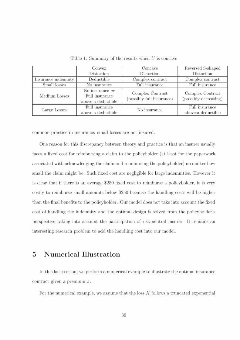
Table 1: Summary of the results when U is concave

ConvexDistortion

ConcaveDistortion

Reversed S-shapedDistortion

Insurance indemnity Deductible Complex contract Complex contract

Small losses No insurance Full insurance Full insurance

Medium LossesNo insurance or

Full insuranceabove a deductible

Complex Contract(possibly full insurance)

Complex Contract(possibly decreasing)

Large LossesFull insurance

above a deductibleNo insurance

Full insuranceabove a deductible

common practice in insurance: small losses are not insured.

One reason for this discrepancy between theory and practice is that an insurer usually

faces a fixed cost for reimbursing a claim to the policyholder (at least for the paperwork

associated with acknowledging the claim and reimbursing the policyholder) no matter how

small the claim might be. Such fixed cost are negligible for large indemnities. However it

is clear that if there is an average $250 fixed cost to reimburse a policyholder, it is very

costly to reimburse small amounts below $250 because the handling costs will be higher

than the final benefits to the policyholder. Our model does not take into account the fixed

cost of handling the indemnity and the optimal design is solved from the policyholder’s

perspective taking into account the participation of risk-neutral insurer. It remains an

interesting research problem to add the handling cost into our model.

5 Numerical Illustration

In this last section, we perform a numerical example to illustrate the optimal insurance

contract given a premium π.

For the numerical example, we assume that the loss X follows a truncated exponential

36

distribution with parameter m = 0.1. The density over [0,M ] is given by

f(x) =me−mx

1− e−mM.

The initial wealth is 15 and we assume that U is the exponential utility U(x) = 1− e−γx

with γ > 0. Indeed, because of the use of exponential utility, the optimal solution does

not depend on the initial wealth W0, as we can see easily from the objective function in

Problem 2.4. We assume that ρ = 0.2.9 Assume that the concave distortion over [0, 1] is

Ta(x) = xa, 0 < a < 1,

and the convex distortion over [0, 1] is

Ta(x) = xa, a > 1.

The reversed S-shaped distortion is similar as the one by Tversky and Kahneman (1992)

and is given by

Ta(x) =xa

(xa + (1− x)a)1

a

, a ∈ (0, 1).

For each of the distortions displayed in Figure 5, we compute the corresponding optimal

shapes of the indemnity for the insured. This corresponds to the three graphs in Panels

A, B and C of Figure 6.

9We take an arbitrary choice of ρ for this section. The proportional safety loading highly dependson the type of insurance. For example for automobile insurance, it will be much lower than that forcatastrophic insurance.

37

0 0.1 0.2 0.3 0.4 0.5 0.6 0.7 0.8 0.9 10

0.1

0.2

0.3

0.4

0.5

0.6

0.7

0.8

0.9

1

T

a=0.7a=0.8a=0.9

0 0.2 0.4 0.6 0.8 10

0.2

0.4

0.6

0.8

1

T

a=1.1a=1.3a=1.5

0 0.1 0.2 0.3 0.4 0.5 0.6 0.7 0.8 0.9 10

0.1

0.2

0.3

0.4

0.5

0.6

0.7

0.8

0.9

1

T

a=0.5a=0.65a=0.8

Panel A Panel B Panel C

Figure 5: Probability Distortions. Panel A is the concave distortion, Panel B is theconvex distortion and Panel C is the reversed S-shaped distortion for different values ofthe parameter a.

The optimal shapes are consistent with the theoretical analysis and with the qualitative

features reported in Table 1. In the case of a convex distortion (Figure 6-Panel A), the

optimum is a deductible contract whose deductible does not depend on the parameter of

the distortion. The premium determines the deductible level which is the only parameter

of the contract. In the case of a concave distortion (Figure 6-Panel B), the optimal

indemnity is clearly concave. Note that the upper limit on indemnity could possibly be

binding (I(X) = X) as it appears in the case when γ = 0.2 and a = 0.9. This suggests

that it would be optimal for a policyholder that has such a distortion to overinsure medium

losses if the indemnity were allowed to exceed the loss amount. This departs from the

standard optimal insurance design for which the constraint I(X) 6 X is automatically

satisfied and for which it is never optimal to overinsure the loss. In the case of the reversed

S-shaped distortion, we observe full insurance for small losses, a decreasing indemnity to

no insurance and then a stop-loss indemnity.

38

Figure 6: There are 3 panels corresponding to the 3 types of distortions considered inthe paper. The 3 graphs correspond to the optimal shapes of the indemnity for π = 3,W0 = 15, ρ = 0.2, an exponential claim with parameter m = 0.1.

0 1 2 3 4 5 6 7 8 9 100

0.5

1

1.5

2

2.5

3

3.5

4

4.5

5

Loss X

Inde

mnit

y I(X

)

Panel A: Convex distortion.

0 1 2 3 4 5 60

0.5

1

1.5

2

2.5

3

3.5

4

4.5

Loss X

γ=0.2, a=0.7γ=0.2, a=0.8γ=0.2, a=0.9Deductible

Panel B: Concave distortion.

0 1 2 3 4 5 6−0.5

0

0.5

1

1.5

2

2.5

3

3.5

4

4.5

Loss X

a=0.5a=0.65a=0.8Deductible

Panel C: Reversed S-shaped distortion.

39

6 Conclusions

In this paper we have derived explicit forms for optimal indemnities for insured behav-

ing as in the RDU framework. In particular the optimal insurance indemnities have been

obtained when the distortion of the RDU-agent is reversed S-shaped, as well as when it

is concave or convex. Comparisons are then drawn toward the end of the paper. Such

comparisons are useful to better understand the effect of the probability distortion on

optimal insurance contracting. Ultimately the goal is to understand how to model human

behavior and what the implications of the model choice are on the insurance market.

This paper makes use of the quantile formulation technique developed by He and

Zhou (2010). Such an advanced tool is needed to construct an optimal solution when the

pointwise optimum does not satisfy the constraints.

A Proof of Theorem 4.1

The proof of Theorem 4.1 is similar to that of Theorem 3.1. It is a consequence of the

following propositions and lemmas, which are the analogues of Proposition 3.1, Lemma

3.1-3.2, Proposition 3.2, and Proposition 3.3.

Proposition A.1. Under Assumptions 3.1, 3.2 and 4.1, let G(·) be any feasible solution

of (7). There exists c ∈ (0, z2(λ)] with the associated Gc(z) such that: (i) Vλ(G(·)) 6

Vλ(Gc(·)); (ii) the equality holds if and only if G(z) = Gc(z), 0 < z < 1.

Lemma A.1. Suppose that Assumptions 3.1, 3.2 and 4.1 hold. Then if λ 6 U ′(W0−π−

F−1X (0+)), then h2(z) < 0 for any z ∈ (0, 1). If λ > T ′(1−)U ′(W0 − π − F−1

X (1−)), then

h2(z) > 0 for any z ∈ (0, 1). If U ′(W0−π−F−1X (0+)) < λ < T ′(1−)U ′(W0−π−F−1

X (1−)),

h2(·) admits a unique root, denoted by z∗(λ), on (0, 1). On (0, z∗(λ)), h2(z) > 0, and on

(z∗(λ), 1), h2(z) < 0.

40

Proposition A.2. Suppose that Assumptions 3.1, 3.2 and 4.1 hold. Then

(i) If λ 6 U ′(W0 − π − F−1X (0+)), then the optimal solution of (7) is

G∗λ(z) = 0, 0 < z < 1. (31)

(ii) If U ′(W0 − π − F−1X (0+)) < λ < T ′(1−)U ′(W0 − π − F−1

X (1−)), then the optimal

solution of (7) is

G∗λ(z) = F−1

X (z)1z6z∗(λ) + F−1X (z∗(λ))1z>z∗(λ), 0 < z < 1. (32)

(iii) If λ > T ′(1−)U ′(W0 − π − F−1X (1−)), then the optimal solution of (7) is

G∗λ(z) = F−1

X (z), 0 < z < 1. (33)

Furthermore, the following function X (λ) :=∫ 1

0G∗

λ(z)dz, 0 < λ < ∞ is continuous on

(0,∞), strictly increasing on [U ′(W0−π−F−1(0+)), T ′(1−)U ′(W0−π−F−1(1−))], and

X (U ′(W0 − π − F−1(0+))) = 0, X (T ′(1−)U ′(W0 − π − F−1(1−))) = E[X ].

Proposition A.3. Suppose that Assumptions 3.1, 3.2, and 4.1 hold. For any 0 6 π 6

min(W0 −M, (1 + ρ)E[X ]), the optimal solution of (6) is

G∗(z) = F−1X (z)1z6c∗ + F−1

X (c∗)1z>c∗, 0 < z < 1, (34)

where c∗ is the unique real number such that∫ 1

0G∗(z)dz = E[X ]− π

1+ρ.

41

References

Arrow, K. J. (1963): Uncertainty and the Welfare Economics of Medical Care, Ameri-

can Economic Review, 53(5), 941–973.

Arrow, K. J. (1971): Essays in the Theory of Risk Bearing. Chicago: Markham.

Barberis, N., and M. Huang (2008): Stocks as Lotteries: The Implications of Proba-

bility Weighting for Security Prices, American Economic Review, 98(5), 2066–2100.

Bernard, C., and M. Ghossoub (2010): Static Portfolio Choice under Cumulative

Prospect Theory, Mathematics and Financial Economics, 2(4), 277 – 306.

Bernard, C., and W. Tian (2009): Optimal Reinsurance Arrangements Under Tail

Risk Measures, Journal of Risk and Insurance, 76(3), 709–725.

Bernard, C., and W. Tian (2010): Optimal Insurance Policies When Insurers Imple-

ment Risk Management Metrics, The Geneva Risk and Insurance Review, 35, 47–80.

Carlier, G., and R.-A. Dana (2003): Core of Convex Distortions of a Probability,

Journal of Economic Theory, 113, 199–222.

Carlier, G., and R.-A. Dana (2005a): Existence and Monotonicity of Solutions to

Moral Hazard Problems, Journal of Mathematical Economics, 41, 826–843.

Carlier, G., and R.-A. Dana (2005b): Rearrangement Inequalities in Non-Convex

Insurance Models, Journal of Mathematical Economics, 41, 483–503.

Carlier, G., and R.-A. Dana (2008): Two-persons efficient risk-sharing and equilibria

for concave law-invariant utilities, Economic Theory, 36(2), 189–223.

Carlier, G., and R.-A. Dana (2011): Optimal demand for contingent claims when

agents have law-invariant utilities, Mathematical Finance, 21(2), 169–201.

42

Chateauneuf, A., R.-A. Dana, and J. Tallon (2000): Optimal risk-sharing rules and

equilibria with Choquet-expected-utility, Journal of Mathematical Economics, 34(2),

191–214.

Cummins, J. D., and O. Mahul (2004): The Demand for Insurance With an Upper

Limit on Coverage, Journal of Risk and Insurance, 71(2), 253–264.

Dana, R.-A., and M. Scarsini (2007): Optimal Risk Sharing with Background Risk,

Journal of Economic Theory, 133(1), 152–176.

Dana, R.-A., andN. Shahidi (2000): Optimal Insurance Contracts under non Expected

Utility, Working Paper, Ceremade, Paris-Dauphine.

Doherty, N., and L. Eeckhoudt (1995): Optimal Insurance Without Expected Util-

ity: The Dual Theory and the Linearity of Insurance Contracts, Journal of Risk and

Uncertainty, 10, 157–179.

Gajek, L., and D. Zagrodny (2004): Optimal Reinsurance under General Risk Mea-

sures, Insurance: Mathematics and Economics, 34, 227–240.

Gollier, C. (1987): The Design of Optimal Insurance Contracts Without the Nonneg-

ativity Constraints on Claims, Journal of Risk and Insurance, 54(2), 314–324.

Gollier, C. (1996): Optimal Insurance of Approximate Losses, Journal of Risk and

Insurance, 63, 369–380.

Gollier, C., and H. Schlesinger (1996): Arrow’s Theorem on the Optimality of

Deductibles: A Stochastic Dominance Approach, Economic Theory, 7, 359–363.

He, X. D., and X. Y. Zhou (2010): Hope, Fear, and Aspiration, Working Paper.

He, X. D., and X. Y. Zhou (2011a): Portfolio Choice under Cumulative Prospect

Theory: An Analytical Treatment, Management Science, 57(2), 315–331.

43

He, X. D., and X. Y. Zhou (2011b): Portfolio Choice via Quantiles, Mathematical

Finance, 21(2), 203–231.

Jin, H. Q., and X. Y. Zhou (2008): Behavioral Portfolio Selection in Continous Time,

Mathematical Finance, 18(3), 385–426.

Jin, H. Q., and X. Y. Zhou (2010): Erratum to ‘Behavioral Portfolio Selection in

Continuous Time’, Mathematical Finance, 20(3), 521–525.

Kaluska, M. (2001): Optimal Reinsurance under Mean-Variance Principles, Insurance:

Mathematics and Economics, 28, 61–67.

Lopes, L. L. (1987): Between Hope and Fear: The Psychology of Risk, Advances in

Experimental Social Psychology, 20, 255–295.

Prelec, D. (1998): The Probability Weighting Function, Econometrica, 66(3), 497–527.

Quiggin, J. (1982): A Theory of Anticipated Utility, Journal of Economic Behavior,

3(4), 323–343.

Quiggin, J. (1991): Comparative Statics for Rank-Dependent Expected Utility Theory,

Journal of Risk and Uncertainty, 4, 339–350.

Quiggin, J. (1993): Generalized Expected Utility Theory - The Rank-Dependent Model.

Kluwer Academic Publishers.

Raviv, A. (1979): The Design of an Optimal Insurance Policy, American Economic

Review, 69(1), 84–96.

Schlesinger, H. (1997): Insurance Demand Without the Expected-Utility Paradigm,

Journal of Risk and Insurance, 64, 19–39.

44

Sung, K., S. Yam, S. Yung, and J. Zhou (2011): Behavioral Optimal Insurance,

Insurance: Mathematics and Economics, forthcoming.

Tversky, A., and C. R. Fox (1995): Weighing Risk and Uncertainty, Psychological

Review, 102(2), 269–283.

Tversky, A., and D. Kahneman (1992): Advances in Prospect Theory: Cumulative

Representation of Uncertainty, Journal of Risk and Uncertainty, 5(4), 297–323.

Yaari, M. (1987): The Dual Theory of Choice under Risk, Econometrica, 55(1), 95–115.

45