optimal time-consistent investment and reinsurance strategies for insurers under heston’s sv model
TRANSCRIPT

Insurance: Mathematics and Economics 51 (2012) 191–203
Contents lists available at SciVerse ScienceDirect
Insurance: Mathematics and Economics
journal homepage: www.elsevier.com/locate/ime
Optimal time-consistent investment and reinsurance strategies for insurersunder Heston’s SV model
Zhongfei Li a,b, Yan Zeng a,∗, Yongzeng Lai ca Lingnan (University) College, Sun Yat-sen University, Guangzhou 510275, PR Chinab Sun Yat-sen Business School, Sun Yat-sen University, Guangzhou 510275, PR Chinac Department of Mathematics, Wilfrid Laurier University, Waterloo, Ontario, Canada, N2L 3C5
a r t i c l e i n f o
Article history:Received May 2011Received in revised formAugust 2011Accepted 9 September 2011
MSC:IM52IE13IB91
Keywords:Investment and reinsurance strategyStochastic volatilityTime-consistencyInsurerMean–variance criterion
a b s t r a c t
This paper considers the optimal time-consistent investment and reinsurance strategies for an insurerunder Heston’s stochastic volatility (SV) model. Such an SV model applied to insurers’ portfolio problemshas not yet been discussed as far as we know. The surplus process of the insurer is approximated bya Brownian motion with drift. The financial market consists of one risk-free asset and one risky assetwhose price process satisfies Heston’s SVmodel. Firstly, a general problem is formulated and a verificationtheorem is provided. Secondly, the closed-form expressions of the optimal strategies and the optimalvalue functions for the mean–variance problem without precommitment are derived under two cases:one is the investment–reinsurance case and the other is the investment-only case. Thirdly, economicimplications and numerical sensitivity analysis are presented for our results. Finally, some interestingphenomena are found and discussed.
© 2011 Elsevier B.V. All rights reserved.
1. Introduction
Due to the facts that reinsurance is an effective way to spreadrisk and that investment is an increasingly important elementin the insurance business, optimal investment and reinsuranceproblems for insurers have drawn great attention in recent years.For example, Browne (1995), Yang and Zhang (2005), Wang(2007) and Xu et al. (2008) studied the optimal investmentstrategies to maximize insurers’ expected exponential utility fromthe terminal wealth under different market assumptions; Baiand Guo (2008), Luo et al. (2008), Luo (2009) and Azcue andMuler (2009) investigated the optimal investment and reinsurancestrategies to minimize the ruin probability of insurers in differentsituations. In addition, some scholars have recently studied theoptimal investment and reinsurance strategies for insurers under
This research is supported by grants from the National Science Foundation forDistinguished Young Scholars (No. 70825002), the National Basic Research Programof China (973 Program, No. 2007CB814902), and ‘‘985 Project’’ of Sun Yat-senUniversity.∗ Corresponding author. Tel.: +86 20 84110516, +86 20 84111989; fax: +86 20
84114823.E-mail addresses: [email protected] (Z. Li), [email protected],
[email protected] (Y. Zeng), [email protected] (Y. Lai).
0167-6687/$ – see front matter© 2011 Elsevier B.V. All rights reserved.doi:10.1016/j.insmatheco.2011.09.002
the mean-variance criterion proposed by Markowitz (1952), seeamong others, Bäuerle (2005), Delong and Gerrard (2007), Bai andZhang (2008), Zeng et al. (2010) and Zeng and Li (2011).
However, two aspects are worthy to be further explored basedon the above-mentioned literature. On the one hand, the priceprocesses of risky assets inmost of the above-mentioned literatureare assumed to follow geometric Brownian motion. Hence, thevolatilities of risky assets are constant or deterministic, which iscontrary to the fact. Stochastic volatility (SV) has been recognizedrecently as an important feature for asset price models. Thereis much literature documenting SV in assets’ returns, such asFrench et al. (1987) and Pagan and Schwert (1990). Meanwhile,SV can be seen as an explanation of many well-known empiricalfindings, such as the volatility smile, the volatility clustering, andthe heavy-tailed nature of return distributions.Many scholars havestudied the optimal investment and/or consumption problemsunder the expected utility criterion with SV models. For example,Zariphopoulou (1999), Fleming and Hernández-Hernández (2003),Chacko and Viceira (2005) and Liu (2007) considered the optimalinvestment and consumption problems under SV models andderived the closed-form expression of the optimal strategies andthe optimal value functions in some situations using the HJBapproach; Zariphopoulou (2001), Pham (2002), Kraft (2005) andTaksar and Zeng (2009) studied the optimal investment problems

192 Z. Li et al. / Insurance: Mathematics and Economics 51 (2012) 191–203
under SV models. Moreover, Korn and Kraft (2001) solved theoptimal investment problems with stochastic interest rates andderived the optimal strategies to maximize the expected utilityfrom the terminal wealth using a stochastic control method;Ferland andWatier (2010) considered amean-variance investmentproblem with the Cox–Ingersoll–Ross (CIR) interest rate in acontinuous-time framework and constructed a mean-varianceefficient portfolio through the solution of backward stochasticdifferential equations. Li and Wu (2009) and Noh and Kim (2010)studied the optimal investment problems with an SV asset priceprocess and a stochastic interest rate to maximize the expectedutility from the terminal wealth.
On the other hand, the optimal strategies of the above-mentioned literature under the mean-variance criterion are nottime-consistent in the sense that, if they are optimal at the initialtime, they are also optimal in any remaining time interval. Thereare two reasons for this. First, the mean-variance criterion lacksthe iterated expectation property; hence, continuous-time andmultiperiod mean-variance problems are time-inconsistent in thesense that the Bellman’s principle of optimality does not hold.Second, the optimal strategies are derived under the assumptionthat the investors precommit themselves not to deviate from thestrategies chosen at the initial time. However, in many situationstime-consistency of strategies is a basic requirement for rationaldecision-makers. Strotz (1956) proposed that time-inconsistentproblems could be handled by a strategy of precommitment ora strategy of time-consistency. Subsequently, Phelps and Pollak(1968), Pollak (1968) and Barro (1999) further considered time-inconsistent problems in different situations. Recently, Björk andMurgoci (2009), Wang and Forsyth (2011), Björk et al. (2010),Basak and Chabakauri (2010), Czichowsky (2010) and Zeng and Li(2011) paidmuch attention to time-inconsistent stochastic controlproblems and aimed at deriving the optimal time-consistentstrategies.
As far as we know, there is little work in the literature onthe optimal portfolio strategies under the mean-variance criterionwith SV models, and only Zeng and Li (2011) have considered theoptimal time-consistent investment and reinsurance strategies forinsurers under themean-variance criterionwith the Black–Scholesmodel. Besides, Heston’s SV model is very popular for optionpricing. Therefore, in this paper, we study the optimal time-consistent investment and reinsurance strategies for insurers withHeston’s SV model. Specifically, the surplus processes of insurersare assumed to follow a Brownian motion with drift; the financialmarket consists of one risk-free asset and one risky asset whoseprice satisfies Heston’s SV model. We first formulate a generalproblem, and provide the corresponding verification theorem.Second, we derive the explicit closed-form expressions of theoptimal time-consistent strategies and the corresponding valuefunctions for themean-variance problemwithout precommitmentunder two cases: the investment–reinsurance case and theinvestment-only case. In the first case, insurers are allowed topurchase proportional reinsurance, acquire new business andinvest in the financial market. In the second case, insurers areonly allowed to invest in the financial market but not to purchaseproportional reinsurance or acquire new business. At the end,some economic implications of our results and sensitivity analysiswith numerical illustrations are presented. This paper has threemain contributions: (i) the optimal portfolio problem under themean-variance criterion with SV models is studied; (ii) the time-inconsistent investment and reinsurance problemswith SVmodelsis considered, and the closed-formexpressions of the optimal time-consistent strategies and the corresponding value functions arederived; (iii) a verification theorem for general problems, includingthe mean-variance problem without precommitment, is provided.
The remainder of this paper is organized as follows. The modeland assumptions are described in Section 2. In Section 3, a generaltime-inconsistent problem is formulated, and the corresponding
verification theorem is provided. In Section 4, the closed-formsolution for the mean-variance problem without precommitmentis derived in two scenarios: the investment–reinsurance caseand the investment-only case. Some economic implications andsensitivity analysis with numerical illustrations are presented inSection 5, and Section 6 presents our conclusions.
2. Model and assumptions
In this paper, we assume that there are no transaction costsor taxes in the financial market or the insurance market, andtrading can be continuous. All stochastic processes introducedbelow are assumed to be well-defined and adapted processes ina given filtered complete probability space (Ω, F , Ftt∈[0,T ], P ),where T is a positive finite constant representing the time horizon;Ftt∈[0,T ] is a filtration; each Ft can be interpreted as theinformation available at time t , and any decision made at time tis based upon such information.
2.1. Surplus process
We assume that the insurer’s surplus process is modeled by adiffusion approximation (DA) model:dR0(t) = µ0 dt + σ0 dW0(t), (1)where µ0 represents the premium return rate of the insurer;σ0 > 0 can be regarded as the volatility of the insurer’s surplus;W0(t) is a one dimensional standard Brownian motion. Readersinterested in how to derive the DA model are referred to Grandll(1991). The DAmodel (1) works well for large insurance portfoliossince each claim is relatively small compared to the size of surplus,and this model has been widely used in the literature, for example,Browne (1995), Promislow and Young (2005), Gerber and Shiu(2006), Bai and Guo (2008), Chen et al. (2010), and so on.
We assume that the insurer can control its insurance risk bypurchasing proportional reinsurance or acquiring new business,for example, by acting as a reinsurer of other insurers (see Bäuerle(2005)). For each t ∈ [0, T ], the proportional reinsurance/newbusiness level is denoted by the value of risk exposure a(t) ∈
[0, +∞). When a(t) ∈ [0, 1], it corresponds to a proportionalreinsurance cover; in this case, the cedent should divert part ofthe premium to the reinsurer at the rate of (1 − a(t))η, whereη ≥ µ0 is the premium return rate of the reinsurer; meanwhile,the insurer pays 100a(t)%while the reinsurer pays the rest 100(1−
a(t))% for each claim occurring at time t . When a(t) ∈ (1, +∞),it corresponds to acquiring new business. The process of riskexposure a(t) : t ∈ [0, T ] is called the reinsurance strategy, andthe DA dynamics for the surplus process associated with such areinsurance strategy a(t) : t ∈ [0, T ] is given bydR(t) = [µ0 − (1 − a(t))η] dt + σ0a(t) dW0(t). (2)
2.2. Financial market
We assume that the financial market consists of one risk-free asset (e.g. a bond or a bank account) and one risky asset(e.g. a stock); the price process S0(t) of the risk-free asset evolvesaccording to the ordinary differential equation (ODE)dS0(t) = r0S0(t) dt, S0(0) = s0 > 0, (3)where r0 > 0 represents the risk-free interest rate; the price pro-cesses S1(t) of the risky asset follows Heston’s SV model
dS1(t) = S1(t)(r0 + λL(t)) dt +
L(t) dW1(t)
,
S1(0) = s1 > 0,
dL(t) = k(θ − L(t)) dt + σL(t) dW2(t),
L(0) = l0 > 0,
(4)

Z. Li et al. / Insurance: Mathematics and Economics 51 (2012) 191–203 193
where λ, k, θ , and σ are all positive constants; W1(t) andW2(t) are twoone-dimensional standardBrownianmotionswithCov(W1(t),W2(t)) = ρt . Moreover, we assume that W0(t) isindependent of W1(t) and W2(t), and we require 2kθ ≥ σ 2
to ensure that zero is not accessible or L(t) is almost surely non-negative.
2.3. Wealth process
During the time horizon [0, T ], the insurer is allowed to dy-namically purchase proportional reinsurance/acquire new busi-ness and invest in the financial market. A trading strategy is apair of stochastic processes denoted by π = (aπ (t), bπ (t))t∈[0,T ],where aπ (t) is the value of risk exposure at time t , and bπ (t) isthe dollar amount invested in the risky asset at time t . The dollaramount invested in the risk-free asset at time t is Xπ (t) − bπ (t),where Xπ (t) is the wealth process associated with the strategyπ . Then Xπ (t) is a solution to the following stochastic differentialequation (SDE):
dXπ (t) = dR(t) + (Xπ (t) − bπ (t))dS0(t)S0(t)
+ bπ (t)dS1(t)S1(t)
= [µ + r0Xπ (t) + ηaπ (t) + λL(t)bπ (t)] dt
+ σ0aπ (t) dW0(t) +
L(t)bπ (t) dW1(t),
Xπ (0) = x0, (5)
where x0 is the wealth at time 0 and µ = µ0 − η.
Definition 1 (Admissible Strategy). Let O := R × R+ and Q :=
[0, T ] × O. For any fixed t ∈ [0, T ], a strategy π = (aπ (s),bπ (s))s∈[t,T ] is said to be admissible if
(i) ∀(x, l) ∈ O, the SDE (5) has a pathwise unique solutionXπ (s)s∈[t,T ] with Xπ (t) = x and L(t) = l;
(ii) ∀s ∈ [t, T ], aπ (s) ≥ 1 and E T
t (|aπ (s)|4 + |bπ (s)|4) ds
<
∞;(iii) ∀ϱ ∈ [1, +∞) and ∀(t, x, l) ∈ Q, Et,x,l
sups∈[t,T ] |Xπ (s)|ϱ
<
∞, where Et,x,l[·] is the condition expectation given Xπ (t) = xand L(t) = l.
In addition, letΠ1(t, x, l) denote the set of all admissible strategieswith respect to (w.r.t.) the initial condition (t, x, l) ∈ Q andΠ2(t, x, l) := π ∈ Π1(t, x, l) : aπ (s) ≡ 1, ∀s ∈ [t, T ].
3. Problem formulation and verification theorem
As far as we know, in the existing literature on optimal invest-ment and/or reinsurance strategies for an insurer under mean-variance criterion, most authors assume that the insurer’s aim isto solve the following problem:
J0(0, x0, l0) = supπ∈Π
E0,x0,l0 [X
π (T )] −γ
2Var0,x0,l0 [X
π (T )]
, (6)
where Π is the corresponding admissible set and γ is the coef-ficient of risk aversion of the insurer. Problem (6) is a static opti-mization problem as one determines the optimal strategyw.r.t. theobjective function set at the initial time 0. The corresponding op-timal strategy of such an optimization problem (6) is only optimalat date 0. In Kryger and Steffensen (2010), Problem (6) is called themean-variance optimization problemwith precommitment in thatE0,x0,l0 [X
π (T )] in the variance term is not updated at subsequentdates. That is, the insurer precommits to herself/himself to the tar-get E0,x0,l0 [X
π (T )]. The corresponding optimal strategy is called theoptimal precommitment strategy, which is time-inconsistent.
However, time-consistency of strategies is a basic requirementof rational decision-making under many situations in practice, and
today’s preference may be different from tomorrow’s preference.We may change our objective function at a future time. There-fore, we need to consider an optimization problem when the ob-jective function changes over the time horizon and to derive acorresponding optimal time-consistent strategy. It is natural to ex-tend the static problem (6) to a dynamic problem as follows: Forany (t, x, l) ∈ Q, the objective function of the insurer is
supπ∈Π
Et,x,l[Xπ (T )] −
γ
2Vart,x,l[Xπ (T )]
. (7)
Here, the insurer wants to find the optimal time-consistentstrategy, i.e., sitting at time t , the optimal strategy derived at time tshould agree with the optimal strategy derived at t + ∆t . Problem(7) is called the mean-variance optimization problem withoutprecommitment, and it is a time-inconsistent problem in the sensethat it does not satisfy the Bellman’s principle of optimality.
In order tomake our verification theoremmoremeaningful andmore suitable for extensive optimization problems,we are going toconsider a general problem. For convenience,we first provide somenotations. Let O0 ⊂ Rn be an open set and O = [0, T ] × O0. Denotethat
C1,2(O) =
φ(t, x) | φ(t, ·) is once continuously
differentiable on [0, T ] and φ(·, x) is twice
continuously differentiable on O0
,
D1,2p (O) =
φ(t, x) | φ(t, x) ∈ C1,2(O) and all once partial
derivatives of φ(·, x) satisfy the polynomial growth
condition on O0
.
Consider the following general problem: for any (t, x, l) ∈ Q,the objective function of the insurer is
supπ∈Π(t,x,l)
f (t, x, l, yπ (t, x, l), zπ (t, x, l)), (8)
and the insurer aims to find the optimal time-consistent strategy,where f : [0, T ] × R4
→ R is a function in D1,2p ([0, T ] × R4),
yπ (t, x, l) = Et,x,l[Xπ (T )], (9)
zπ (t, x, l) = Et,x,l[(Xπ (T ))2], (10)and Π(t, x, l) is the corresponding admissible set at state (t, x, l).
Problem (8) reduces to our concernedmean-variance optimiza-tion problem without pre-commitment (7), if
f (t, x, l, y, z) = y −γ
2(z − y2). (11)
In addition, if we set f to be different forms, problem (8) hasdifferent objective functions and different meanings. For example,problem (8) becomes the mean-variance optimization problemwithout precommitment but with state-dependent risk aversioncoefficient γ (t, x, l), if
f (t, x, l, y, z) = y −γ (t, x, l)
2(z − y2),
and it reduces to the mean-standard derivation optimizationproblem without precommitment but with state-dependent riskaversion coefficient, if
f (t, x, l, y, z) = y −γ (t, x, l)
2(z − y2)
12 .
Definition 2. For any fixed chosen initial state (t, x, l) ∈ Q,consider an admissible strategy π∗(t, x, l). Choose three fixed realnumbers a > 0, b, and τ > 0 and define the following strategy:
πτ (s, x, l) =
(a, b), for t ≤ s < t + τ , (x, l) ∈ O,
π∗(s, x, l), for t + τ ≤ s < T , (x, l) ∈ O.

194 Z. Li et al. / Insurance: Mathematics and Economics 51 (2012) 191–203
If
limτ→0
inff π∗
(t) − f πτ (t)τ
≥ 0, ∀(a, b) ∈ O,
then π∗(t, x, l) is called an equilibrium strategy, and the equilib-rium value function is defined by
V (t, x, l) = f (t, x, l, yπ∗
(t, x, l), zπ∗
(t, x, l)),
where f π (t) = f (t, x, l, yπ (t, x, l), zπ (t, x, l)).Based on Definition 2, equilibrium strategies are time-
consistent. Therefore, we assume that at any state (t, x, l) ∈ Q, theaim of the insurer is to find an equilibrium strategy and the corre-sponding equilibrium value function of the optimization problem(8). Hereafter, the equilibrium strategy π∗ and the correspondingvalue function V (t, x, l) of problem (8) are called the optimal time-consistent strategy and the optimal value function of (8) in this pa-per. Before giving the verification theorem, we define a variationaloperator. For any φ(t, x, l) ∈ C1,2(Q), letAπφ(t, x, l) = φt(t, x, l) + φx(t, x, l)
× [µ + r0x + ηaπ (t) + λlbπ (t)]
+ φl(t, x, l)k(θ − l) +12φxx(t, x, l)
× [σ 20 a
π (t)2 + lbπ (t)2]
+12φll(t, x, l)σ 2l + φxl(t, x, l)ρσ lbπ (t),
∀(t, x, l) ∈ Q.
Theorem 1 (Verification Theorem). For the optimization prob-lem (8), if there exist three real value functions F(t, x, l),G(t, x, l),H(t, x, l) ∈ D1,2
p (Q) satisfying the following conditions: ∀(t, x, l)∈ Q,
supπ∈Π(t,x,l)
AπF(t, x, l) − ξπ (t, x, l) = 0, (12)
F(T , x, l) = f (T , x, l, x, x2), (13)
Aπ∗
G(t, x, l) = 0, G(T , x, l) = x, (14)
Aπ∗
H(t, x, l) = 0, H(T , x, l) = x2, (15)
and
π∗:= arg sup
π∈Π(t,x,l)AπF(t, x, l) − ξπ (t, x, l) , (16)
then V (t, x, l) = F(t, x, l), yπ∗
(t, x, l) = G(t, x, l), zπ∗
(t, x, l) =
H(t, x, l), and π∗ is the optimal time-consistent strategy, where
ξπ (t, x, l) := ft + fx[µ + r0x + ηaπ (t) + λlbπ (t)] + flk(θ − l)
+Uπ1
2[σ 2
0 aπ (t)2 + lbπ (t)2]
+Uπ2
2σ 2l + Uπ
3 ρσ lbπ (t), (17)
Uπ1 := fxx + 2fxyyπ
x + 2fxzzπx + fyy(yπ
x )2 + fzz(zπx )2
+ 2fyzyπx z
πx , (18)
Uπ2 := fll + 2fylyπ
l + 2fzlzπl + fyy(yπ
l )2 + fzz(zπl )2
+ 2fyzyπl z
πx , (19)
Uπ3 := fxl + fxyyπ
l + fxzzπl + fylyπ
x + fzlzπx + fyyyπ
x yπl
+ fyzyπx z
πl + fyzyπ
l zπx + fzzzπ
x zπl (20)
and f = f (t, x, l, y, z), yπ= yπ (t, x, l), zπ
= zπ (t, x, l).The proof of this theorem is given in the Appendix.
4. Mean-variance problem without precommitment
Themean-variance criterion is a very important objective func-tion in modern portfolio theory, and our goal is to derive the
closed-form expression of the optimal time-consistent strategyand the optimal value function satisfying the Verification Theo-rem 1. We focus on the mean-variance problem without precom-mitment in this section. Specifically, we consider two cases: one isthe investment–reinsurance case, and the other is the investment-only case. In the first case, the insurer is allowed to invest in thefinancial market, purchase proportional reinsurance, and acquirenew business; in the second case, the insurer is only allowed to in-vest in the financialmarket. Correspondingly, at any state (t, x, l) ∈
Q, the admissible strategy set for the first case and the second caseare Π1(t, x, l) and Π2(t, x, l), respectively. According to (11), wehave
ft = fx = fl = fxx = fxy = fxz = fyz = fxl= fyl = fzl = fzz = fll = 0,
fy = 1 + γ y, fyy = γ , fz = −γ
2.
(21)
4.1. Solution to the investment–reinsurance case
In this subsection, we study the investment–reinsurance caseand derive the optimal time-consistent strategy and the optimalvalue function.
In the following, we construct the corresponding solution tothe investment–reinsurance case. Assume that there are three realfunctions F(t, x, l), G(t, x, l) and H(t, x, l) satisfying the conditionsgiven in Theorem 1 and Uπ
1 > Fxx(t, x, l) for all (t, x, l) ∈ Q and allπ ∈ Π1(t, x, l). According to Theorem 1 and inserting the partialderivatives in (21) into (17)–(20), we have
Uπ∗
1 = γG2x , Uπ∗
2 = γG2l , Uπ∗
3 = γGxGl,
ξπ∗
(t, x, l) =γ
2G2x [σ
20 a
π∗
(t)2 + lbπ∗
(t)2]
+γ
2G2l σ
2l + γGxGlρσ lbπ∗
(t)
(22)
with G = G(t, x, l) for short. Moreover, (8), (11) and Theorem 1imply that
F(t, x, l) = V (t, x, l) = f (t, x, l, yπ∗
, zπ∗
)
= Et,x,l[Xπ∗
(T )]
−γ
2
Et,x,l[Xπ∗
(T )2] − (Et,x,l[Xπ∗
(T )])2
= G(t, x, l) −γ
2[H(t, x, l) − G(t, x, l)2]. (23)
Therefore
H(t, x, l) = G(t, x, l)2 +2γ
[G(t, x, l) − F(t, x, l)]. (24)
In addition, by differentiating the expression inside the bracketof (12)w.r.t. aπ (t) and bπ (t), respectively, and by applying (22), wecan obtain the optimal strategy as follows:
π∗= (aπ∗
(t), bπ∗
(t)), aπ∗
(t) = −ηFx
σ 20 (Fxx − γG2
x),
bπ∗
(t) = −λFx + ρσ Fxl − γ ρσGxGl
Fxx − γG2x
.
(25)
Substituting (25) into (12) and (14), we have
Ft + Fx(µ + r0x) + Flk(θ − l) +12Fllσ 2l −
γ
2G2l σ
2l
−η2F 2
x
2σ 20 (Fxx − γG2
x)−
(λFx + ρσ Fxl − γ ρσGxGl)2l
2(Fxx − γG2x)
= 0, (26)

Z. Li et al. / Insurance: Mathematics and Economics 51 (2012) 191–203 195
Gt + Gx(µ + r0x) + Glk(θ − l) +12Gllσ
2l
−η2Fx
σ 20 (Fxx − γG2
x)
Gx −
GxxFx2(Fxx − γG2
x)
−(λFx + ρσ Fxl − γ ρσGxGl)l
Fxx − γG2x
λGx
+ ρσGxl −(λFx + ρσ Fxl − γ ρσGxGl)Gxx
2(Fxx − γG2x)
= 0. (27)
Since (26)–(27) and the boundary conditions of F(t, x, l) andG(t, x, l) are linear in x and l, it is logical to assume that
F(t, x, l) = A(t)x +A(t)γ
l +A(t)γ
,
A(T ) = 1, A(T ) = A(T ) = 0,
(28)
G(t, x, l) = α(t)x +α(t)γ
l +α(t)γ
,
α(T ) = 1, α(T ) = α(T ) = 0.(29)
The partial derivatives are
Ft = Atx +At
γl +
At
γ, Fx = A(t), Fl =
A(t)γ
,
Gt = αtx +αt
γl +
αt
γ, Gx = α(t), Gl =
α(t)γ
.
Inserting the above partial derivatives into (25)–(27), we obtain
aπ∗
(t) =ηA(t)
γ σ 20 α(t)2
, bπ∗
(t) = −λA(t) − γ ρσα(t)α(t)
γ α(t)2, (30)
Atx +At
γl +
At
γ+ A(t)(µ + r0x) +
A(t)γ
k(θ − l) −α(t)2σ 2l
2γ
+η2A(t)2
2γ σ 20 α(t)2
+[λA(t) − ρσα(t)α(t)]2l
2γα(t)2= 0, (31)
αtx +αt
γl +
αt
γ+ α(t)(µ + r0x) +
α(t)γ
k(θ − l) +η2A(t)
γ σ 20 α(t)
+[λA(t) − ρσα(t)α(t)]λl
γα(t)= 0. (32)
By separating the variables with x, with l and without x, lrespectively, we can derive the following system of ODEs:
At + A(t)r0 = 0, A(T ) = 1, (33)
At − kA(t) −α(t)2σ 2
2
+[λA(t) − ρσα(t)α(t)]2
2α(t)2= 0, A(T ) = 0, (34)
At + A(t)µγ + kθ A(t) +η2A(t)2
2σ 20 α(t)2
= 0, A(T ) = 0, (35)
αt + α(t)r0 = 0, α(T ) = 1, (36)
αt − kα(t) +λ2A(t) − λρσα(t)α(t)
α(t)= 0, α(T ) = 0, (37)
αt + α(t)µγ + kθα(t) +η2A(t)σ 20 α(t)
= 0, α(T ) = 0. (38)
Solving the above ODEs, we have
A(t) = α(t) = er0(T−t), (39)
A(t) =A e2(k+λρσ)(t−T )
k + 2λρσ
−(2A + B) e(k+λρσ)(t−T )
λρσ+ δ ek(t−T )
+Ck, (40)
A(t) =Akθ(1 − e2(k+λρσ)(t−T ))
2(k + λρσ)(k + 2λρσ)
−kθ(2A + B)(1 − e(k+λρσ)(t−T ))
λρσ(k + λρσ)
+ δθ(1 − ek(t−T )) +γµ
r0(er0(T−t)
− 1)
+
η2
2σ 20
+ θC
(T − t), (41)
α(t) =λ2
(k + λρσ)(1 − e(k+λρσ)(t−T )), (42)
α(t) =λ2kθ
(k + λρσ)2(e(k+λρσ)(t−T )
− 1) +γµ
r0( er0(T−t)
− 1)
+
λ2kθ
(k + λρσ)+
η2
σ 20
(T − t), (43)
where
A =λ4σ 2(1 − ρ2)
2(k + λρσ)2, B =
λ3ρσ
(k + λρσ),
C =λ2
2− (A + B), δ =
2A + Bλρσ
−A
k + 2λρσ−
Ck.
(44)
Note that if ρ, k+λρσ , or k+2λρσ is equivalent to 0, then A(t),A(t), α(t), and α(t) given in (40)–(43) are also valid in the sense oflimit. For example, when k + λρσ = 0,
α(t) = λ2(T − t), (45)
α(t) =µγ
r0(er0(T−t)
− 1) +λ2kθ2
(T − t)2 +η2
σ 20(T − t), (46)
the right hand side of the above two formulas are the limits of (42)and (43) as k + λρσ tends to 0.
According to (24) and (28)–(29), we obtain
H(t, x, l) =
α(t)x +
α(t)γ
l +α(t)γ
2
+2γ 2
(α(t) − A(t))l + α(t) − A(t)
, (47)
where A(t), A(t), A(t), α(t), α(t) and α(t) are given by (39)–(43).Inserting (39) into (30), we obtain the optimal strategy
π∗= (aπ∗
(t), bπ∗
(t)), aπ∗
(t) =η
γ σ 20er0(t−T ),
bπ∗
(t) =
k + λρσ e(k+λρσ)(t−T )
γ (k + λρσ)λ er0(t−T ),
if k + λρσ = 0,λ
γ[1 + λρσ(t − T )] er0(t−T ),
if k + λρσ = 0.
(48)
Based on the above derivation, it is not difficult to verifythat F(t, x, l), G(t, x, l), H(t, x, l) and π∗ given by (28)–(29), and(47)–(48), respectively, indeed satisfy the conditions in Theorem 1.Thus, we have the following theorem.

196 Z. Li et al. / Insurance: Mathematics and Economics 51 (2012) 191–203
Theorem 2. For the investment–reinsurance problem, the optimaltime-consistent strategy is given by (48); the corresponding optimalvalue function is given by
F(t, x, l) = x er0(T−t)+
A(t)γ
l +A(t)γ
,
where A(t), A(t) are given by (40) and (41); and the expectedterminal wealth under the optimal strategy is given by
G(t, x, l) = x er0(T−t)+
α(t)γ
l +α(t)γ
,
where α(t), α(t) are given by (42)–(43).
Remark 1. (i) The optimal strategyπ∗ is a deterministic functionand it does not depend on the wealth process Xπ∗
(t) or thevolatility of the risky asset L(t);
(ii) the premium rate of the insurer µ0 has no impact on theoptimal strategy π∗ but has impact on the optimal valuefunction F(t, x, l);
(iii) the parameters of the risky asset have no influence on the op-timal reinsurance strategy aπ∗
(t), and the parameters of in-surance market have no influence on the optimal investmentstrategy bπ∗
(t).
Remark 2. According to (42)–(43) and (45)–(46), it is not difficultto find that a(t) and a(t) are nonnegative in [0, T ], which impliesthat G(t, x, l) ≥ x er0(T−t), and that G(t, x, l) increases w.r.t l butdecreases w.r.t γ .
In addition, according to (34), (37), (40) and (42), we obtain
α(t) − A(t) = A T
tek(t−s)
e(k+λρσ)(s−T )− 1
2ds
+λ2
2k(1 − ek(t−T )). (49)
According to (35) and (38), we have
α(t) − A(t) = kθ T
t(α(s) − A(s)) ds +
η2
2σ 20(T − t). (50)
Because A given by (44) is nonnegative, it is easy to show thatα(t) − A(t) ≥ 0 and α(t) − A(t) ≥ 0. According to the secondequation of (23), we have
Vart,,x,l[Xπ∗
(T )] =2γ
[G(t, x, l) − F(t, x, l)]
=2γ 2
(α(t) − A(t))l + α(t) − A(t)
=
m(t, l)2
γ 2, (51)
wherem(t, l)2
2= l
A
T
tek(t−s)
e(k+λρσ)(s−T )− 1
2ds
+λ2
2k(1 − ek(t−T ))
+ Akθ
T
t
T
sek(s−u)
e(k+λρσ)(u−T )− 1
2du ds
+λ2θ
2
T
t(1 − ek(s−T )) ds +
η2
2σ 20(T − t). (52)
According to Theorem 2, we know that ∀(t, x, l) ∈ Q,
Et,x,l[Xπ∗
(T )] = G(t, x, l) = x er0(T−t)+
α(t)γ
l +α(t)γ
, (53)
and the last equation of (51) implies that
1γ
=
Vart,,x,l[Xπ∗
(T )]
m(t, l). (54)
Substituting (54) into (53), we have
Et,x,l[Xπ∗
(T )] = x er0(T−t)
+α(t)l + α(t)
m(t, l)
Vart,,x,l[Xπ∗
(T )]. (55)
Remark 3. (55) is known as the efficient frontier of the invest-ment–reinsurance problem at state (t, x, l) in modern portfoliotheory. The efficient frontier is also a straight line in the mean-standard deviation plane, no matter at which state.
4.2. Solution to the investment-only case
In this subsection, we consider the investment-only case andderive the explicit optimal value function and the optimal time-consistent strategy. In this case, the value of risk exposure aπ (t) ≡
1, ∀t ∈ [0, T ] and the set of all admissible strategies is denotedby Π2(t, x, l), ∀(t, x, l) ∈ Q. When an admissible strategy π ∈
Π(t, x, l) is adopted, the correspondingwealth processXπ (t) is thesolution of the following SDE:
dXπ (t) = [µ0 + r0Xπ (t) + λL(t)bπ (t)] dt
+ σ0 dW0(t) +
L(t)bπ (t) dW1(t). (56)
Similar to the investment–reinsurance case, for the investment-only case we can also derive the optimal strategy π∗ and threereal value function F(t, x, l), G(t, x, l) and H(t, x, l) satisfying theconditions in Theorem 1, which are described as follows:
π∗= (1, bπ∗
(t)), bπ∗
(t) = bπ∗
(t), (57)
F(t, x, l) = x er0(T−t)+
A(t)γ
l +B(t)γ
, (58)
G(t, x, l) = x er0(T−t)+
α(t)γ
l +β(t)γ
, (59)
H(t, x, l) =
x er0(T−t)
+α(t)γ
l +β(t)γ
2
+2γ 2
(α(t) − A(t))l + β(t) − B(t)
, (60)
where A(t) and α(t) are given by (40) and (42), respectively;whereas, B(t) and β(t) satisfy the following ODEs:
Bt + µ0γ er0(T−t)+ kθ A(t) −
γ 2σ 20
2e2r0(T−t)
= 0,
B(T ) = 0,(61)
βt + γµ0 er0(T−t)+ kθα(t) = 0, β(T ) = 0, (62)
and they are given by
B(t) =Akθ(1 − e2(k+λρσ)(t−T ))
2(k + λρσ)(k + 2λρσ)
−kθ(2A + B)(1 − e(k+λρσ)(t−T ))
λρσ(k + λρσ)+ θC(T − t)
+ δθ(1 − ek(t−T )) +γµ0(er0(T−t)
− 1)r0
−γ 2σ 2
0 (e2r0(T−t)− 1)
4r0, (63)

Z. Li et al. / Insurance: Mathematics and Economics 51 (2012) 191–203 197
β(t) =λ2kθ
(k + λρσ)2(e(k+λρσ)(t−T )
− 1)
+γµ0( er0(T−t)
− 1)r0
+λ2kθ(T − t)(k + λρσ)
. (64)
Similarly, if ρ, k+λρσ , or k+2λρσ is equivalent to 0, then B(t)and β(t) given in (63)–(64) are also valid in the sense of limit. Forexample, when k + λρσ = 0,
β(t) =µ0γ
r0( er0(T−t)
− 1) +λ2kθ2
(T − t)2. (65)
The right hand side of (65) is the limit of (64) as k + λρσ tendsto 0.
Hence, according to Theorem 1, we have the following result:
Theorem 3. For the investment-only problem, the optimal strategyis given by (57); the optimal value function is given by (58); and theexpected terminal wealth under the optimal strategy is given by (59).
Remark 4. The optimal investment strategy bπ∗
(t) of theinvestment-only problem is the same as that of the invest-ment–reinsurance problem. This property implies that the optimalinvestment and reinsurance strategy canbe separated, and the eco-nomic implications of the optimal investment strategy stated afterTheorem 2 apply to this model as well.
Remark 5. According to (64) and (65), we can derive that β(t) isnonnegative in [0, T ]. According to Remark 2, we have α(t) ≥ 0,∀t ∈ [0, T ]. Hence, G(t, x, l) ≥ x er0(T−t), and G(t, x, l) also in-creases w.r.t l but decreases w.r.t γ .
In addition, by (49), (61) and (62), we can obtain
β(t) − B(t) = Akθ T
t
T
sek(s−u)
e(k+λρσ)(u−T )− 1
2du ds
+λ2θ
2
T
t(1 − ek(s−T )) ds +
γ 2σ 20
4r0( e2r0(T−t)
− 1). (66)
It is easy to show that β(t) − B(t) ≥ 0. According to (49) and (66),we can derive
Vart,,x,l[Xπ∗
(T )] =2γ
[G(t, x, l) − F(t, x, l)]
=2γ 2
(α(t) − A(t))l + β(t) − B(t)
=
n(t, l)2
γ 2+
σ 20
2r0( e2r0(T−t)
− 1), (67)
wheren(t, l)2
2= l
A
T
tek(t−s)
e(k+λρσ)(s−T )− 1
2ds
+λ2
2k(1 − ek(t−T ))
+ Akθ
T
t
T
sek(s−u)
e(k+λρσ)(u−T )− 1
2du ds
+λ2θ
2
T
t(1 − ek(s−T )) ds. (68)
Theorem 3 implies that ∀(t, x, l) ∈ Q,
Et,x,l[X π∗
(T )] = G(t, x, l) = x er0(T−t)+ l
α(t)γ
+β(t)γ
, (69)
and the second equation of (67) leads to
1γ
=
Vart,,x,l[Xπ∗
(T )] −σ 20
2r0( e2r0(T−t) − 1)
n(t, l). (70)
Substituting (70) into (69), we obtain
Et,x,l[Xπ∗
(T )] = x er0(T−t)
+α(t)l + β(t)
n(t, l)
Vart,,x,l[Xπ∗
(T )] −σ 20 ( e2r0(T−t) − 1)
2r0, (71)
where Vart,,x,l[Xπ∗
(T )] ≥σ 20
2r0( e2r0(T−t)
− 1) is guaranteed by(67). (71) is known as the efficient frontier of the investment-onlyproblem at state (t, x, l) in modern portfolio theory. The efficientfrontier is no longer a straight line but a hyperbola in the mean-standard deviation plane. It is a straight line only when σ0 = 0.This reveals that due to the existence of the volatility σ0 of theinsurer’s surplus process, the risk of insurance business cannot becompletely hedged by only investment.
Corollary 1. The optimal value function of the investment–reinsurance problem is larger than that of the investment-onlyproblem. In other words, reinsurance can increase the insurer’s mean-variance utility.Proof. According to Theorems 2 and 3, it follows that
F(t, x, l) − F(t, x, l) =A(t) − B(t)
γ
=12γ
T
t
η
σ0− γ σ0 er0(T−s)
2
ds ≥ 0.
5. Sensitivity analysis and numerical illustration
In this section, we study the effect of parameters on theoptimal strategies and the optimal value functions and providesome numerical examples to illustrate the effects. For thefollowing numerical illustrations, unless otherwise stated, thebasic parameters are given by µ0 = 0.5, σ0 = 1, η = 0.8, γ = 0.6,r0 = 0.05, λ = 1.5, k = 2, θ = 0.03, σ = 1.5, ρ = 0.3, T = 10(years), t = 0, x0 = 1 and l0 = 1.
5.1. Analysis of optimal strategies
In this subsection, we provide some sensitivity analysis on theeffect of the parameters on the optimal strategies. Meanwhile,some numerical examples are provided to illustrate our results.
(1) According to (48), we can derive that ∂aπ∗(t)
∂η> 0, ∂aπ
∗(t)
∂t >
0, ∂aπ∗(t)
∂σ0< 0, ∂aπ
∗(t)
∂γ< 0 and ∂aπ
∗(t)
∂r0< 0, which imply that the
optimal reinsurance strategy aπ∗
(t) increases w.r.t the premiumreturn rate of the reinsurer η and time t , but decreases w.r.t thevolatility of the surplus process σ0, the coefficient of risk aversionof the insurer γ and the risk-free interest rate r0. We provide somenumerical illustration in Fig. 1.
In Fig. 1, (a) shows that the optimal reinsurance strategy aπ∗
(t)decreases as the coefficient of risk aversion of the insurer γincreases; i.e., the more risk aversion the insurer is, the morereinsurance is purchased or the less new business is acquired; (b)indicates that the optimal reinsurance strategy aπ∗
(t) decreasesw.r.t the risk-free interest rate r0, i.e., the insurer should purchasemore reinsurance or acquire less new business, if the risk-freeinterest rate r0 becomes larger; (c) demonstrates that the optimalreinsurance strategy aπ∗
(t) decreases w.r.t the volatility of thesurplus process σ0, i.e., if the risk of the insurance businessdecreases, the insurer will purchase less reinsurance or acquiremore new business; (d) illustrates that the larger the premiumreturn rate of the reinsurer η, the larger the optimal reinsurancestrategy aπ∗
(t), which implies that the insurer will purchase lessreinsurance or acquire more new business, if the premium returnrate of the reinsurer η increases.
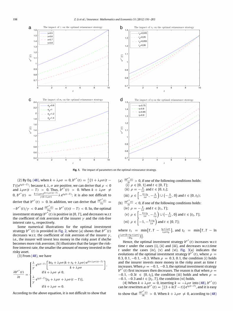
198 Z. Li et al. / Insurance: Mathematics and Economics 51 (2012) 191–203
a b
c d
Fig. 1. The impact of parameters on the optimal reinsurance strategy.
(2) By Eq. (48), when k + λρσ = 0, bπ∗
(t) =λγ[1 + λρσ(t −
T )] er0(t−T ); because k, λ, σ are positive, we can derive that ρ < 0
and λρσ(t − T ) > 0. Thus, bπ∗
(t) > 0. When k + λρσ =
0, bπ∗
(t) =k+λρσ e(k+λρσ)(t−T )
γ (k+λρσ)λ er0(t−T )
; it is also not difficult to
derive that bπ∗
(t) > 0. In addition, we can derive that ∂bπ∗(t)
∂γ=
−bπ∗
(t)/γ < 0 and ∂bπ∗(t)
∂r0= bπ∗
(t)(t − T ) < 0. So, the optimal
investment strategy bπ∗
(t) is positive in [0, T ], and decreases w.r.tthe coefficient of risk aversion of the insurer γ and the risk-freeinterest rate r0, respectively.
Some numerical illustrations for the optimal investmentstrategy bπ∗
(t) is provided in Fig. 2, where (a) shows that bπ∗
(t)decreases w.r.t. the coefficient of risk aversion of the insurer γ ,i.e., the insurer will invest less money in the risky asset if she/hebecomes more risk aversion; (b) illustrates that the larger the risk-free interest rate, the smaller the amount of money invested in therisky asset.
(3) From (48), we have
∂bπ∗
(t)∂t
=
λ
γer0(t−T )
kr0 + λρσ(k + r0 + λρσ) e(k+λρσ)(t−T )
k + λρσ
,
if k + λρσ = 0,λ
γer0(t−T )
[r0 + λρσ + λρσ(t − T )],
if k + λρσ = 0.
According to the above equation, it is not difficult to show that
(a) ∂bπ∗(t)
∂t > 0, if one of the following conditions holds:(i) ρ ∈ [0, 1] and t ∈ [0, T ];(ii) ρ = −
kλσ
and t ∈ [0, t1];
(iii) ρ ∈
−
k+r0λσ
, − kλσ
∪
−
kλσ
, 0and t ∈ [0, t2);
(b) ∂bπ∗(t)
∂t < 0, if one of the following conditions holds:(iv) ρ = −
kλσ
and t ∈ [t1, T ];
(v) ρ ∈
−
k+r0λσ
, − kλρ
∪
−
kλσ
, 0and t ∈ [t2, T ];
(vi) ρ ∈
−1, − k+r0
λσ
and t ∈ [0, T ];
where t1 = minT , T −
r0+λρσ
λρσ r0
, and t2 = min
T , T − ln
λρσ(k+r0+λρσ)
−kr0
.
Hence, the optimal investment strategy bπ∗
(t) increases w.r.ttime t under the cases (i), (ii) and (iii), and decreases w.r.t.timet under the cases (iv), (v) and (vi). Fig. 3(a) indicates theevolutions of the optimal investment strategy bπ∗
(t), where ρ =
0.3, 0.1, −0.1, −0.3. When ρ = 0.3, 0.1, the condition (i) holdsand the insurer invests more money in the risky asset as time tincreases.When ρ = −0.1, −0.3, the optimal investment strategybπ∗
(t) first increases then decreases. The reason is that when ρ =
−0.1, −0.3t ∈ [0, t2], the condition (iii) holds and when ρ =
−0.1, −0.3 and t ∈ [t2, T ], the condition (vi) holds.(4) When k + λρσ = 0, inserting k = −λρσ into (48), bπ∗
(t)can be rewritten as bπ∗
(t) =λγ[1+ k(T − t)] er0(t−T ), and it is easy
to show that ∂bπ∗(t)
∂k > 0. When k + λρσ = 0, according to (48)

Z. Li et al. / Insurance: Mathematics and Economics 51 (2012) 191–203 199
a b
Fig. 2. The impact of γ and r0 on the optimal investment strategy.
ba
Fig. 3. The impact of ρ and k on the optimal investment strategy.
we have
∂bπ∗
(t)∂k
=λ2σ er0(t−T )
γ (k + λρσ)2ρ1 − [1 + (k + λρσ)(T − t)] e(k+λρσ)
;
it is not difficult to obtain the following result:
(i) ∂bπ∗(t)
∂k > 0, if ρ ∈ (0, 1] and k ∈ (0, +∞), or ρ < 0 andk ∈ (0, −λρσ);
(ii) ∂bπ∗(t)
∂k = 0, if ρ = 0;
(iii) ∂bπ∗(t)
∂k < 0, if ρ < 0 and k ∈ (−λρσ, +∞).
Therefore, the optimal investment strategy bπ∗
(t) increases ask increases when ρ ∈ (0, 1] and k ∈ (0, +∞), or ρ < 0 and k ∈
(0, −λρσ ]; the optimal investment strategy bπ∗
(t) is invariable ask becomes large when ρ = 0; the optimal investment strategybπ∗
(t) decreases w.r.t k when ρ < 0 and k ∈ (−λρσ, +∞). InFig. 3(b), the insurer invests more money in the risky asset as theparameter k increases, which is due to ρ = 0.3.
However, the relations between the optimal investmentstrategy bπ∗
(t) and the parameters λ and σ are not easy to obtain.We provide some numerical examples (See Fig. 4).
5.2. Analysis of optimal value functions
In this subsection, we analyze the effect of the insurancemarketparameters µ0, η, and σ0 on the optimal value functions. ByTheorems 2 and 3, we have
∂F(t, x, l)∂µ0
=∂ F(t, x, l)
∂µ0=
γ
r0(er0(T−t)
− 1),
∂F(t, x, l)∂σ0
= −η2
σ 30(T − t),
∂F(t, x, l)∂η
=η
σ 20(T − t) −
γ
r0( er0(T−t)
− 1),
∂ F(t, x, l)∂σ0
= −γ 2σ0( e2r0(T−t)
− 1)2r0
.
According to the above equations, we know that (i) the optimalvalue functions F(t, x, l) and F(t, x, l) increase w.r.t. the premiumreturn rate of the insurer µ0; (ii) the optimal value functionsF(t, x, l) and F(t, x, l) decrease w.r.t. the volatility of the surplusprocess σ0; (iii) the optimal value function F(t, x, l) decreasesw.r.t.
η when η ∈µ0,
γ σ 20 ( er0(T−t)
−1)r0(T−t)
and increases w.r.t. η when η ∈ γ σ 2
0 ( er0(T−t)−1)
r0(T−t) , +∞.
Without loss of generality, we only provide the evolutions ofthe optimal value functions w.r.t. the parameters of the insurancemarket at the initial time 0. In Fig. 5, (a) shows that the twooptimal value functions increase as the premium return rate ofthe insurer µ0 becomes larger, i.e., the larger the premium returnrate of the insurer µ0, the larger the two optimal value functions;(b) denotes that the two optimal value functions decrease whenthe risk of the surplus process increases; (c) indicates that underthe investment–reinsurance case, the optimal value function is

200 Z. Li et al. / Insurance: Mathematics and Economics 51 (2012) 191–203
a b
Fig. 4. The impact of λ and σ on the optimal investment strategy.
a b
c
Fig. 5. The impact of the insurance market parameters on the optimal value functions.
not a monotonic function w.r.t the premium return rate of thereinsurer η. As the premium return rate of the reinsurer ηincreases, the optimal value function first decreases, and thenincreases. That is, both lower and higher premium return ratesof the reinsurer will lead to higher optimal utilities. In addition,from (a) and (b), we know that the optimal value function underthe investment–reinsurance case is larger than that under the
investment-only case, which is consistent with the result ofCorollary 1.
6. Conclusions
In this paper, we have investigated an insurer’s optimal time-consistent investment and reinsurance strategies under Heston’s

Z. Li et al. / Insurance: Mathematics and Economics 51 (2012) 191–203 201
SV model. The surplus process of the insurer is assumed to fol-low a diffusion approximation model. The financial market isassumed to consist of one risk-free asset and one risky asset.The price process of the the risky asset is assumed to fol-low the Heston’s SV model. We have first formulated a gen-eral time-inconsistent problemwhich includes the mean-variancewithout precommitment problem, and have provided the corre-sponding verification theorem. Then, we have solved the mean-variance without precommitment problem for two cases: theinvestment–reinsurance case and the investment-only case; andwe have derived the closed-form expressions of the optimal time-consistent strategies, the optimal value functions and the effectivefrontiers. Finally, we have provided some sensitivity analysis of theoptimal strategies and the optimal value functions and some nu-merical illustration. The main findings are as follows: (i) the opti-mal value functions are linear functions w.r.t. the current wealthx and the current volatility l of the risky asset; (ii) the optimal in-vestment strategy and the optimal reinsurance strategy are deter-ministic, and they are all independent of the wealth process; (iii)the optimal function of the investment–reinsurance case is largerthan that under the investment-only problem, i.e., reinsurance canincrease the mean-variance utility.
As far as we know, there is no work on the optimal invest-ment and reinsurance problem for mean-variance insurers withstochastic volatility in the literature. Especially, we have aimed toderive the optimal time-consistent strategy. However, our pa-per also has some limits: (i) we only consider the optimal time-consistent strategy and do not study the optimal precommitmentstrategy; (ii) we only consider the simplest but important stochas-tic volatility model; (iii) the price process of the risky asset is con-tinuous andwithout jumps; (iv) the time horizon T is pregiven andfixed. In future works, we will relax these assumptions and con-sider more general cases.
Appendix
In this appendix, we first give a lemmawhichwill be used in theproof of Theorem 1.
Lemma 1. Under the assumptions given at the beginning of Sec-tion 2.2, if φ(t, x, l) ∈ D1,2
P (Q), then ∀(t, x, l) ∈ Q and ∀π ∈
Π1(t, x, l), the following integrals are martingales.
Mπ1 (t, x, l) =
T
tφx(s, Xπ , L(s))σ0aπ (s) dW0(s),
Mπ2 (t, x, l) =
T
tφx(s, Xπ , L(s))
L(s)bπ (s) dW1(s),
Mπ3 (t, x, l) =
T
tφl(s, Xπ , L(s))σ
L(s) dW2(s).
Proof. Let (t, x, l) ∈ Q and π ∈ Π1(t, x, l). According to thedefinition of the admissible strategy, we have
∀ϱ ∈ [1, +∞), Et,x,l
sup
s∈[t,T ]
|Xπ (s)|ϱ
< ∞. (72)
In addition, the dynamics of L(t) given by (4) satisfies the lineargrowth and Yamada andWatanabe conditions, which implies that
∀ϱ ∈ [1, +∞), Et,x,l
sup
s∈[t,T ]
|L(s)|ϱ
< +∞. (73)
Because of φ(t, x, l) ∈ D1,2P (Q), there exist two constants κ > 0
and p ≥ 1 such that
|φx(t, x, l)| ≤ κ(1 + |x|p + |l|p). (74)
According to (72)–(74), we have
Et,x,l
T
t
φx
L(s)bπ (s)
2 ds
≤ Et,x,l
T
t
φx
L(s)
4+ bπ (s)4
ds
≤ Et,x,l
T
t
φ8x + L(s)4 + bπ (s)4
ds
≤ Et,x,l
T
t
κ8(1 + |Xπ (s)|p + |L(s)|p)8
+ L(s)4 + bπ (s)4ds
< ∞ (75)
with φx = φx(s, Xπ (s), L(s)) for short.Similarly, we can prove that
Et,x,l
T
t|φx(s, Xπ (s), L(s))σ0aπ (s)|2 ds
< ∞, (76)
Et,x,l
T
t
φl(s, Xπ (s), L(s))σL(s)
2 ds
< ∞. (77)
By (75)–(77) we know thatMπi (t, x, l), i = 1, 2, 3 aremartingales.
Proof of Theorem 1. The proof consists of three steps.(i) Consider an arbitrary admissible strategy π ∈ Π1(t, x, l).Firstly, we claim that if there exists a real value function
Y (t, x, l) ∈ D1,2p (Q) such that ∀(t, x, l) ∈ Q,
AπY (t, x, l) = 0, (78)Y (T , x, l) = x, (79)
then
Y (t, x, l) = yπ (t, x, l). (80)
In fact, according to Itô’s formula and Eq. (5), we have
Yπ (t) = Yπ (T ) −
T
tdYπ (s)
= Yπ (T ) −
T
tAπYπ (s) ds −
T
t
Yπx (s)
σ0aπ (s) dW0(s)
+
L(s)bπ (s) dW1(s)
+ Yπ
l (s)σL(s) dW2(s)
, (81)
with Yπ (t) = Y (t, Xπ (t), L(t)) for short. Using Lemma 1 andtaking the conditional expectation on the both sides of the aboveformula, we have
Y (t, x, l) = Et,x,l[Yπ (t)] = Et,x,l[Xπ (T )] = yπ (t, x, l).
Similarly, by replacing Y and y by Z and z, respectively we canshow that if there exists a real value function Z(t, x, l) ∈ D1,2
p (Q)such that ∀(t, x, l) ∈ Q
AπZ(t, x, l) = 0, (82)
Z(T , x, l) = x2, (83)
then
Z(t, x, l) = zπ (t, x, l). (84)
For brevity, we denote Zπ (t) = Z(t, Xπ (t), L(t)), ξπ (t) =
ξπ (t, Xπ (t), L(t)), Fπ (t) = F(t, Xπ (t), L(t)) and f π (t) = f (t,Xπ (t), L(t), Yπ (t), Zπ (t)).

202 Z. Li et al. / Insurance: Mathematics and Economics 51 (2012) 191–203
Secondly, given Y (t, x, l) satisfying (78)–(79) and Z(t, x, l)satisfying (82)–(83), we can derive an expression for f π (T ),i.e. formula (87) below.
From (80) and (84), it follows that
f (t, Xπ (t), L(t), yπ (t, Xπ (t), L(t)), zπ (t, Xπ (t), L(t)))
= f π (t). (85)
Since f ∈ D1,2p ([0, T ]×R4), by Itô’s formula and the Eq. (5) we have
f π (T ) = f π (t) +
T
tdf π (s)
= f π (t) +
T
t[f πy (s)AπYπ (s)
+ f πz (s)AπZπ (s) + ξπ (s)] ds +
T
t
(f π
x (s)
+ f πy (s)Yπ
x (s) + f πz (s)Zπ
x (s))(σ0aπ (s) dW0(s)
+
L(s)bπ (s) dW1(s))
+ (f πl (s) + f π
y (s)Yπl (s) + f π
z (s)Zπl (s))
× σL(s) dW2(s)
. (86)
Substituting (78) and (82) into (86), we obtain
f π (T ) = f π (t) +
T
tξπ (s) ds +
T
t
(f π
x (s) + f πy (s)Yπ
x (s)
+ f πz (s)Zπ
x (s))(σ0aπ (s) dW0(s)
+
L(s)bπ (s) dW1(s)) + (f π
l (s)
+ f πy (s)Yπ
l (s) + f πz (s)Zπ
l (s))σL(s) dW2(s)
. (87)
Thirdly, based on (87), we show that ∀(t, x, l) ∈ Q,
F(t, x, l) ≥ supπ∈Π(t,x,l)
f (t, x, l, yπ (t, x, l), zπ (t, x, l)). (88)
Applying Itô’s formula to F(t, x, l) and using (5), we have
Fπ (t) = Fπ (T ) −
T
tdFπ (s)
= Fπ (T ) −
T
tAπFπ (s) ds −
T
t
Fπx (s)
σ0aπ (s) dW0(s)
+
L(s)bπ (s) dW1(s)
+ Fπ
l (s)σL(s) dW2(s)
. (89)
Moreover, (12) implies that ∀(t, x, l) ∈ Q, AπF(t, x, l) ≤
ξπ (t, x, l), then
Fπ (t) ≥ Fπ (T ) −
T
tξπ (s) ds −
T
t
Fπx (s)
σ0aπ (s) dW0(s)
+
L(s)bπ (s) dW1(s)
+ Fπ
l (s)σL(s) dW2(s)
. (90)
(13) implies Fπ (T ) = f π (T ), then substituting (87) into (90), wehave
Fπ (t) ≥ f π (t) +
T
t
f πx (s) + f π
y (s)Yπx (s) + f π
z (s)Zπx (s)
− Fπx (s)
σ0aπ (s) dW0(s) +
L(s)bπ (s) dW1(s)
+
f πl (s) + f π
y (s)Yπl (s) + f π
z (s)Zπl (s)
− Fπl (s)
σL(s) dW2(s)
. (91)
According to Lemma 1, taking conditional expectation on bothsides of (91) and thereafter supremum over Π(t, x, l), we obtain(88).
(ii) Consider the specific admissible strategy π∗.Firstly, according to the assumption of Theorem 1, functions
G(t, x, l) and H(t, x, l) satisfy the conditions of the two claims inpart (i) with the strategy π∗, hence G(t, x, l) = yπ∗
(t, x, l) andH(t, x, l) = zπ∗
(t, x, l).Secondly, for the specific strategy π∗, the inequalities (90) and
(91) become equations. Hence we have
Fπ∗
(t) = f π∗
(t) +
T
t
f π∗
x (s) + f π∗
y (s)Yπ∗
x (s) + f π∗
z (s)Zπ∗
x (s)
− Fπ∗
x (s)
σ0aπ∗
(s) dW0(s) +
L(s)bπ∗
(s) dW1(s)
+
f π∗
l (s) + f π∗
y (s)Yπ∗
l (s) + f π∗
z (s)Zπ∗
l (s)
− Fπ∗
l (s)σL(s) dW2(s)
. (92)
By Lemma 1 and taking conditional expectation on both sides of(92), we have
F(t, x, l) = f (t, x, l, yπ∗
(t, x, l), zπ∗
(t, x, l))
≤ supπ∈Π(t,x,l)
f (t, x, l, yπ (t, x, l), zπ (t, x, l)). (93)
(92) together with (88) finally gives
F(t, x, l) = supπ∈Π(t,x,l)
f (t, x, l, yπ (t, x, l), zπ (t, x, l)). (94)
This means that π∗ is the optimal strategy and the supremum isgiven by F(t, x, l).
(iii) Prove π∗ is indeed an equilibrium control strategy.For any πτ defined in Definition 2, replacing T by t + τ and π
by πτ in (87), we have
f πτ (t + τ) = f πτ (t) +
t+τ
tξπτ (s) ds
+
t+τ
t
(f πτ
x (s) + f πτy (s)Yπτ
x (s)
+ f πτz (s)Zπτ
x (s))(σ0aπτ (s) dW0(s)
+
L(s)bπτ (s) dW1(s))
+ (f πτl (s) + f πτ
y (s)Yπτl (s) + f πτ
z (s)Zπτl (s))
× σL(s) dW2(s)
. (95)
Replacing T by t + τ and π by π∗ in (90), we have
Fπ∗
(t) ≥ Fπ∗
(t + τ) −
t+τ
tξπ∗
(s) ds
−
t+τ
t
Fπ∗
x (s)σ0aπ∗
(s) dW0(s)
+
L(s)bπ∗
(s) dW1(s)
+ Fπ∗
l (s)σL(s) dW2(s)
. (96)
According to the definition of πτ , we have f πτ (t+τ) = Fπ∗
(t+τ).Then inserting (95) into (96), we obtain
Fπ∗
(t) ≥ f πτ (t) +
t+τ
tξπτ (s)ds −
t+τ
tξπ∗
(s) ds
−
t+τ
t
Fπ∗
x (s)σ0aπ∗
(s) dW0(s)
+
L(s)bπ∗
(s) dW1(s)

Z. Li et al. / Insurance: Mathematics and Economics 51 (2012) 191–203 203
+ Fπ∗
l (s)σL(s) dW2(s)
+
t+τ
t
(f πτ
x (s)
+ f πτy (s)Yπτ
x (s) + f πτz (s)Zπτ
x (s))(σ0aπτ (s) dW0(s)
+
L(s)bπτ (s) dW1(s))
+ (f πτl (s) + f πτ
y (s)Yπτl (s) + f πτ
z (s)Zπτl (s))
× σL(s) dW2(s)
. (97)
Because of Fπ∗
(t) = f π∗
(t) and taking conditional expectation onboth sides of (97), we have
f π∗
(t) ≥ f πτ (t)
+ Et,x,l
t+τ
tξπτ (s) ds −
t+τ
tξπ∗
(s) ds
. (98)
The above formula implies that
limτ→0
inff π∗
(t) − f πτ (t)τ
≥ 0.
References
Azcue, P., Muler, N., 2009. Optimal investment strategy to minimize the ruinprobability of an insurance company under borrowing constraints. Insurance:Mathematics and Economics 44, 26–34.
Bai, L.H., Guo, J.Y., 2008. Optimal proportional reinsurance and investment withmultiple risky assets and no-shorting constraint. Insurance: Mathematics andEconomics 42, 968–975.
Bai, L.H., Zhang, H.Y., 2008. Dynamic mean-variance problem with constrained riskcontrol for the insurers. Mathematical Methods of Operations Research 68,181–205.
Barro, R.J., 1999. Ramseymeets Laibson in the neoclassical growthmodel. QuarterlyJournal of Economics 114, 1125–1152.
Basak, S., Chabakauri, G., 2010. Dynamic mean-variance asset allocation. Review ofFinancial Studies 23, 2970–3016.
Bäuerle, N., 2005. Benchmark andmean-variance problems for insurers.Mathemat-ical Methods of Operations Research 62, 159–165.
Björk, T., Murgoci, A., 2009. A general theory of Markovian time inconsis-tent stochastic control problems. Working paper, Stockholm School ofEconomics. Available at: http://econtent.essec.fr/mediabanks/ESSEC-PDF/Enseignement%20et%20Recherche/Enseignement/Departement/seminaire/Finance/2008-2009/Tomas_Bjork-Seminaire.pdf.
Björk, T., Murgoci, A., Zhou, X.Y., 2010. Mean variance portfolio optimiza-tion with state dependent risk aversion. Working paper. Available at:http://www.wu.ac.at/it/other/vgsf/activities/seminar/bjoerk10.pdf.
Browne, S., 1995. Optimal investment policies for a firm with a random riskprocess: exponential utility and minimizing probability of ruin. Mathematicsof Operations Research 20, 937–958.
Chacko, G., Viceira, L.M., 2005. Dynamic consumption and portfolio choice withstochastic volatility in incomplete markets. The Review of Financial Studies 8,1369–1402.
Chen, S.M., Li, Z.F., Li, K.M., 2010. Optimal investment–reinsurance for an insurancecompany with VaR constraint. Insurance: Mathematics and Economics 47,144–153.
Czichowsky, C., 2010. Time-consistent mean-variance portfolio selection indiscrete and continuous time. Working paper. Available at: http://www.nccr-finrisk.uzh.ch/media/pdf/wp/WP661_D1.pdf.
Delong, Ł., Gerrard, R., 2007. Mean-variance portfolio selection for a non-life insurance company. Mathematical Methods of Operations Research 66,339–367.
Ferland, R., Watier, F., 2010. Mean-variance efficiency with extended CIR interestrates. Applied Stochastic Models in Business and Industry 26, 71–84.
Fleming, W.H., Hernández-Hernández, D., 2003. An optimal consumption modelwith stochastic volatility. Finance and Stochastics 7, 245–262.
French, W.E., Schwert, G.W., Stambaugh, R.F., 1987. Expected stock returns andvolatility. Journal of Financial Economics 19, 3–29.
Gerber, H.U., Shiu, E.S.W., 2006. On optimal dividends: from reflection to refraction.Journal of Computational and Applied Mathematics 186, 4–22.
Grandll, J., 1991. Aspects of risk theory. Springer-Verlag, New York.Korn, R., Kraft, H., 2001. A stochastic control approach to portfolio problems
with stochastic interest rates. SIAM Journal on Control and Optimization 40,1250–1269.
Kraft, H., 2005. Optimal portfolios and Heston’s stochastic volatility model: anexplicit solution for power utility. Quantitative Finance 5, 303–313.
Kryger, E.M., Steffensen, M., 2010. Some solvable portfolio problemswith quadraticand collective objectives. Working paper. Available at: http://papers.ssrn.com/sol3/papers.cfm?abstract_id=1577265.
Li, J.Z., Wu, R., 2009. Optimal investment problem with stochastic interest rate andstochastic volatility: maximizing a power utility. Applied Stochastic Models inBusiness and Industry 25, 407–420.
Liu, J., 2007. Portfolio selection in stochastic environment. The Review of FinancialStudies 20, 1–39.
Luo, S.Z., 2009. Ruin minimization for insurers with borrowing constraints. NorthAmerican Actuarial Journal 12, 143–174.
Luo, S.Z., Taksar, M., Tsoi, A., 2008. On reinsurance and investment for largeinsurance portfolios. Insurance: Mathematics and Economics 42, 434–444.
Markowitz, H.M., 1952. Portfolio selection. Journal of Finance 7, 77–91.Noh, E.J., Kim, J.H., 2010. An optimal portfolio model with stochastic volatility and
stochastic interest rate. Journal of Mathematical Analysis and Applications 375,510–522.
Pagan, A.R., Schwert, G.W., 1990. Alternativemodels for conditional stock volatility.Journal of Econometrics 45, 267–290.
Pham, H., 2002. Smooth solutions to optimal investment models with stochasticvolatilities andportfolio constraints. AppliedMathematics andOptimization 46,55–78.
Phelps, E.S., Pollak, R.A., 1968. On second-best national saving and game-equilibrium growth. Review of Economic Studies 35, 185–199.
Pollak, R.A., 1968. Consistent planning. Review of Economic Studies 35, 201–207.Promislow, S.D., Young, V.R., 2005. Minimizing the probability of ruin when
claims follow Brownian motion with drift. North American Actuarial Journal 9,109–128.
Strotz, R., 1956. Myopia and inconsistency in dynamic utility maximization. Reviewof Economic Studies 23, 165–180.
Taksar, M.I., Zeng, X.D., 2009. A general stochastic volatility model and op-timal portfolio with explicit solutions. Working paper. Available at:http://www.math.missouri.edu/~zeng/pub/ageneral.pdf.
Wang, J., Forsyth, P.A., 2011. Continuous time mean variance asset allocation:a time-consistent strategy. European Journal of Operational Research 209,184–201.
Wang, N., 2007. Optimal investment for an insurer with exponential utilitypreferences. Insurance: Mathematics and Economics 40, 77–84.
Xu, L., Wang, R.M., Yao, D.J., 2008. On maximizing the expected terminalutility by investment and reinsurance. Journal of Industrial and ManagementOptimization 4, 801–815.
Yang, H.L., Zhang, L.H., 2005. Optimal investment for insurer with jump-diffusionrisk process. Insurance: Mathematics and Economics 37, 615–634.
Zariphopoulou, T., 1999. Optimal investment and consumption models with non-linear stock dynamics. Mathematical Methods of Operations Research 50,271–296.
Zariphopoulou, T., 2001. A solution approach to valuation with unhedgeable risks.Finance and Stochastics 5, 61–82.
Zeng, Y., Li, Z.F., 2011. Optimal time-consistent investment and reinsurancepolicies formean-variance insurers. Insurance:Mathematics and Economics 49,145–154.
Zeng, Y., Li, Z.F., Liu, J.J., 2010. Optimal strategies of benchmark and mean-varianceportfolio selection problems for insurers. Journal of Industrial andManagementOptimization 6, 483–496.