optimal thresholds in accounting recognition...
TRANSCRIPT

Optimal Thresholds in Accounting Recognition Standards
Pingyang Gao∗
The University of Chicago Booth School of Business
September, 2017
Abstract
This paper investigates the design of recognition thresholds in accounting standards. In
statistics, a threshold classifies evidence to balance two types of recognition errors weighted
by their respective costs to a decision maker. In accounting recognition standards, a threshold
induces firms to respond strategically and thus affects the very distribution of evidence the
threshold classifies. With this strategic effect, the optimal recognition threshold is determined
by not only the decision maker’s loss function but also the transaction’s features. We compare
the optimal threshold’s properties under the statistical and strategic approaches, provide their
respective empirical predictions, and discuss the limitations of using a statistical approach to
guide accounting standard setting.
JEL recognition: M41, M45, G28, G38
Key Words: Thresholds, Evidence Management, Accounting Standard Setting, Statis-
tical Inference∗I am grateful for comments from Mark Bagnoli, Qi Chen, Doug Diamond, Phil Dybvig, Alex Frankel,
Mathew Gentzkow, Michael Gibbs, Robert Gibbons, Milt Harris, Zhiguo He, Mirko Heinle, Steve Huddart,
Christian Laux (discussant), Volker Laux, Christian Leuz, Canice Prendergast, Haresh Sapra, Doug Skinner,
Jack Stecher, Hao Xue, and participants of Basel accounting workshop, and the accounting workshops at
CKGSB, Duke, INSEAD, Purdue, Southwest University of Economics and Finance, the University of Chicago,
University of Graz, UC Davis and the organizational economics workshop at MIT. I also thank Jinzhi Lu for
able research assistance. All errors are my own. This work is supported by the Centel Foundation/Robert P.
Reuss Faculty Research Fund at the University of Chicago Booth School of Business.

1 Introduction
This paper presents a model to study the design of recognition thresholds in accounting stan-
dards when firms can influence accounting evidence. Many recognition standards involve a
choice from two treatments, such as capitalizing v.s. expensing, sales v.s. secured borrow-
ing, operating leases v.s. capital leases, off-balance-sheet v.s. on-balance-sheet, and so on.
Recognition thresholds specify the strength of evidence required for a preferred accounting
treatment. To make the research question concrete, consider revenue recognition as an ex-
ample. Accountants collect and analyze evidence to assess the probability that the firm has
earned revenue from a transaction. This probability is then compared with a threshold P set
by the revenue recognition standard to determine whether revenue is recognized. This paper
is interested in the optimal design of threshold P . What economic forces determine P? Is
50% a reasonable benchmark? If it becomes more costly for firms to influence evidence, how
does the optimal level of P change?
These seem to be basic questions in setting recognition standards, yet they have received
only limited attention in the prior literature. An explanation for the lack of research on
this seemingly important question is not obvious. One possibility is that threshold design
has been perceived as an immediate application of the well-established statistical approach
and thus does not require further research in accounting. For example, one might liken the
thresholds that qualify a lease transaction as an operating or capital lease to thresholds in a
clinical test that confirm or refute the diagnosis of a disease. Under this statistical approach,
a higher threshold reduces the undue optimism error at the expense of increasing the false
alarm error. The optimal threshold balances these two types of recognition errors according
to their respective costs to the decision maker.
However, threshold design in accounting standards differs from its counterpart in clinical
tests in at least one crucial aspect: the threshold choice in an accounting standard influences
the very distribution of accounting evidence the threshold actually classifies. A change in
the threshold for diagnosing a cancer does not affect the protein content of cells of patients.
In contrast, a change in the term requirements for recognizing capital leases, say from 75%
to 60%, is likely to induce lessees and lessors to structure the lease terms in their contracts
1

differently, resulting in a different distribution of lease terms. Empirical evidence about such
strategic responses has been compiled in the accounting literature, including, among others,
Imhoff and Thomas (1988) (for leases), Lys and Vincent (1995) (for merger and acquisition),
Engel, Erickson, and Maydew (1999) (for hybrid securities), and Dechow and Shakespear
(2009) (for securitization). Moreover, the use of accounting-motivated transactions has long
been a major concern for standard setters and regulators. For example, in its report to the
Congress on the financial reporting of off-balance sheet arrangements, the first recommenda-
tion the Securities and Exchange Commission (the SEC) makes is "to discourage transactions
and transaction structures primarily motivated by accounting and reporting concerns, rather
than economics" (see SEC (2005)). We use the broad term "evidence management" to refer
to firms’activities that influence a transaction’s accounting evidence.
In this paper we examine the optimal design of recognition thresholds in the presence of
evidence management. The paper’s main result is that the optimal threshold in a strategic
approach, which takes into account the firm’s strategic response through evidence manage-
ment, differs markedly from its counterpart in a statistical approach. The optimal probability
threshold in a statistical approach is determined solely by the costs of recognition errors to
the decision maker, while its counterpart in a strategic approach is also affected by the fine
details of the transaction under consideration. To illustrate, consider a revenue recognition
standard when the decision-making costs of premature and delayed recognition of revenue are
the same. The statistical approach predicts that the probability threshold P for recognizing
revenue is 50%, but the strategic approach predicts that it is different from 50% in general.
Moreover, it can be either higher or, perhaps surprisingly, lower than 50%, even though the
manager has a one-sided incentive to inflate evidence in the model. The exact conditions
for each case to prevail depend on the transaction’s details, such as the link between the
transaction’s economic substance and its accounting evidence and this link’s vulnerability to
the manager’s influence.
The intuition for the main result lies in the two distinct effects a threshold has on recogni-
tion errors. On one hand, for any given evidence, a higher threshold reduces a report’s undue
optimism error and increases the false alarm error simultaneously. This statistical effect is
well-understood in the statistical literature. On the other hand, a threshold affects evidence
2

management that, in turn, affects the distribution of evidence and thus recognition errors.
This strategic effect involves the specifics of the transaction under consideration and behaves
differently from the statistical effect. Since the optimal threshold takes into account both the
statistical and strategic effects, it is qualitatively different from its statistical benchmark.
The intuition for the result that the optimal probability threshold in the presence of
inflatory evidence management can be either higher or lower than its statistical benchmark is
as follows. In the model, since evidence management reduces the report’s value for decision-
making, the threshold is designed to discourage evidence management. Whether this entails a
higher or lower threshold, however, depends on the sign of the strategic effect (the threshold’s
effect on evidence management). It turns out that the strategic effect is not monotonic: a
higher threshold initially increases and then reduces evidence management. Therefore, the
optimal threshold is higher than the statistical benchmark if, and only if, a higher threshold
reduces evidence management.
The non-monotonicity of the threshold’s effect on evidence management can be demon-
strated by considering two extremes of setting a threshold. If the threshold is set so low
that everyone can clear it without evidence management, there will be no costly evidence
management. On the other hand, if the threshold is set so high that no one can clear it even
with costly evidence management, there will be no evidence management, either. Therefore,
whenever the threshold affects evidence management, the relation is not monotonic.
To further understand the interaction of threshold design and recognition errors, we study
the threshold design when the standard setter is concerned about maximizing the accounting
report’s ex post value to the decision maker, that is, the value assessed after evidence is
presented. The standard setter takes the evidence as given at the time of choosing the
threshold but has rational expectations about evidence management that has influenced the
distribution of the observed evidence. The optimal probability threshold in this case is the
same as in the statistical benchmark and does not depend on the details of the transaction.
Therefore, it is the threshold’s effect on evidence management, rather than the rational
expectations about evidence management, that distinguishes the strategic from the statistical
approach to threshold design.
This paper’s main antecedent is Dye (2002) who has formalized a tractable framework to
3

study threshold design in the shadow of evidence management. The manager can influence
the mapping from state to evidence and the standard setter chooses a threshold to influence
the mapping from evidence to recognition. Gao (2013b) elaborates this two-step represen-
tation of accounting measurement and suggests its potential for studying various accounting
measurement issues. For example, Gao (2013a) uses this representation to study conser-
vatism. Using this representation, Dye (2002) demonstrates a clear distinction between an
offi cial and a shadow standard, describes conditions for a creep of offi cial standards over time,
and characterizes the dynamic evolution of both the offi cial and shadow standards when the
standard setter is sophisticated or naive and when the distribution of projects is exogenous
or endogenous. In Section 4.2, we explain how this paper differs from Dye (2002) in both
their main results and the economic forces behind the results.
A few other papers have also studied threshold design. Magee (2006) studies threshold
design in a setting in which the manager communicates information about the second mo-
ment of the distribution of his signal in the absence of opportunistic evidence management.
Mittendorf (2010) studies the role of audit thresholds in the misreporting of private informa-
tion. The commitment to tolerating misreporting within the materiality threshold makes the
threat of punishing egregious misreporting above the threshold more effective. Fan and Zhang
(2012) study a model in which managers could exert private efforts to improve the precision
of evidence and use the model to provide justification for conservatism. Laux and Stocken
(2017) show that standards and enforcement can either be complements or substitutes. In
their model the board incorporates rational expectations about the manager’s evidence man-
agement in designing his compensation contract, which in turn affects the manager’s benefit
of receiving a preferred treatment and thus his incentive of evidence management.
The issue of setting evidence thresholds is also studied in the legal literature in the context
of designing the burden of proof (e.g., Kaplow (2011)). In that literature, the manipulation
of evidence is a lesser concern, partly because of the adversary adjudication system. In
addition, the evidence threshold works exclusively through the ex ante incentive effect on
primary activities in Kaplow (2011), whereas in this paper, the threshold’s dual effects on ex
ante evidence management and the ex post statistical effi ciency of decision-making are the
key tension.
4

The paper is also related to the literature on the value of communication, as recently
surveyed in, e.g., Beyer, Cohen, Lys, and Walther (2010), Ewert and Wagenhofer (2012), and
Stocken (2013). In my model the misreporting is costly, the receiver has no commitment,
and there is no transfer between the sender and the receiver. The major departure from this
literature is that my model focuses on the design of the ex ante communication protocol or
the accounting standard that governs the mapping from evidence to the report.
The rest of the paper proceeds as follows. Section 2 describes the model. Section 3 solves
the model and characterizes the optimal threshold. Section 4 considers several extensions.
Section 5 offers some empirical implications. Section 6 concludes.
2 Model
The baseline model has three players, a standard setter, a manager, and a stakeholder. Each
moves once in the following sequences.
1. At date 0, the standard setter chooses a recognition threshold T . The state ω is drawn
by Nature but not observed by anyone.
2. At date 1, the manager engages in unobservable evidence managementm that influences
a transaction’s accounting evidence t.
3. At date 2, evidence t, whose distribution is determined by both ω and m, is realized.
A recognition report r is generated by comparing evidence t with threshold T.
4. At date 3, the stakeholder observes report r and makes a decision d. ω and d jointly
determine the payoffs of the stakeholder and the manager, v(ω, d) and u(ω, d), respec-
tively.
The model is comprised of two parts. The first part depicts a simple decision-making
setting that creates demand for information. The second part elaborates the recognition
process that generates the information.
5

2.1 The demand for information
To focus on the design of accounting standards, we create the demand for information by
assuming an exogenous conflict of interest between the stakeholder (user of information)
and the manager (the producer of information). The state of nature, denoted as ω, is a
transaction’s economic substance. It is either good (G) with probability qG or bad (B) with
probability qB ≡ 1−qG, i.e., ω ∈ {G,B}. It is chosen by Nature at date 0 and not observable
to anyone. At date 3, the stakeholder observes an accounting recognition report r ∈ {g, b}
about the state and makes a binary decision d(r) ∈ {0, 1} to maximize her expected payoff
Eω[v(ω, d)|r]. The expectation is taken with respect to the stakeholder’s information set that
will be specified later. Without loss of generality we assume
LG ≡ v(G, 1)− v(G, 0) > 0, and LB ≡ v(B, 0)− v(B, 1) > 0. (Assumption 1)
Assumption 1 states that with complete information the stakeholder prefers decision d = 1
to d = 0 if and only if the state is good. With incomplete information about state ω, the
stakeholder uses report r as an information source for her decision-making. LG and LB
measure the value of this information to her.
The manager, however, does not always share the stakeholder’s interest. His payoff,
denoted as u(ω, d), is always higher when the stakeholder chooses d = 1, which is equivalent
to assuming
δω ≡ u(ω, 1)− u(ω, 0) > 0, for ω ∈ {G,B}. (Assumption 2)
δω indexes the manager’s preference for d = 1 in state ω.1 This conflict of interest mo-
tivates the manager to engage in evidence management, as will be described in the next
subsection. We assume that nothing is contractible in this setting so as to focus on the role
of financial reporting in a decision-making setting.
Examples that fit this generic setting are common. The stakeholder’s decision d can be
whether to finance a firm’s project (d = 1) or not (d = 0). LG is the NPV of a viable project
1The alternative assumption that the manager prefers d = 0 to d = 1 in both states does not changethe main results qualitatively. What is necessary is the existence, not the direction, of the misalignment ofinterest. In addition, δω is indexted to ω so that the manager’s preference could be state-contingent. Forexample, it allows the manager to prefer decision 1 more in the good state than in the bad state, i.e., δG > δB .
6
and LB the absolute value of the negative NPV of an unprofitable project. For another
example, d could be whether to foreclose a loan or not. LG captures the cost of foreclosing a
good loan and LB of continuing a bad one. Yet another example of the binary decision can be
whether to replace a manager or not. LG is the cost of removing an able manager and LB of
keeping an incompetent one. While in all three examples information about the underlying
state is useful for the stakeholder, the manager prefers financing the project, continuing the
loan, and keeping the job, regardless of the underlying state. Thus, Assumption 1 and 2 are
descriptive of these settings.
2.2 The supply of information through accounting recognition
We turn to the second part of the model and describe the accounting recognition process that
relates report r to state ω through the two-step representation of accounting measurement.
An accounting standard is a mapping from evidence t to report r, while the manager can
influence the mapping from state ω to evidence t. To make this process concrete, consider a
stylized example of revenue recognition. The economic substance ω is whether revenue from
a transaction has been earned (and realizable) or not. Revenue recognition is a preferred
treatment for the manager (r = g). Between ω and r, we introduce a notion of transaction
characteristics or evidence t. Examples of evidence include payment collectability and/or
product delivery (after proper normalization). The revenue recognition standard is then
modeled as a mapping from evidence t to report r. For example, revenue is recognized (r = g)
if and only if product is delivered and payment is collectible (t ≥ T ). Relative to this standard
T , one requiring that product be delivered and cash be received implies a higher threshold,
while one requiring only product delivery implies a lower threshold. The manager can present
favorable evidence of product delivery by either fabricating warehouse records (accounting
manipulation) or adopting tactics of channel stuffi ng (real activity manipulation). Figure 1
illustrates this process.
7

state (ω) − evidence︸ ︷︷ ︸evidence management
(t) − report (r)︸ ︷︷ ︸standard design
− decision(d)
Figure 1 : a two-step representaion of accounting measurement
Now we formalize this recognition process. It is decomposed to two steps: one from
the state to the evidence and the other from the evidence to the report. The model’s key
friction lies in the first step: evidence t depends on both the state and the manager’s evidence
management. In the absence of the latter, evidence t is drawn from a differentiable density
distribution function fω(t) > 0 over [t, t̄] with corresponding cumulative density function
Fω(t). fω(t) satisfies the strict monotone likelihood ratio property (MLRP) and thus a higher
t is good news about the state (Milgrom (1981)).
However, at date 1 before knowing ω the manager can take an unobservable action m
to "improve" the distribution of evidence. m captures all activities the manager engages in
to influence evidence t and is broadly referred to as evidence management. Specifically, we
assume that with manipulation m, the evidence distribution becomes f̃ω(t;m):
f̃ω(t;m) =
fG(t) if ω = G
mfG(t) + (1−m)fB(t) if ω = B,m ∈ [0, 1].(1)
Evidence managementm improves the evidence distribution because, as it can be verified,
for any m1 > m2,f̃B(t;m1)
f̃B(t;m2)is (weakly) increasing in t and F̃B(t;m1) is better than F̃B(t;m2)
in the sense of FOSD (first-order stochastic dominance). Note that m does not affect the
evidence of the good state (i.e., f̃G(t;m) = fG(t)). This is a simplification that stacks
us against finding a non-monotonic relation between the optimal threshold and evidence
management. It will be relaxed in Section 4.3.
m costs the manager cC(m) privately. C(m) has the standard properties of a cost function.
It is increasing and convex with C(0) = C′(0) = 0 and cC
′(1) is suffi ciently large to assure
an interior m in equilibrium. Further, ddm [ C
′
C′′ ] = (C′′)2−C′C′′′
(C′′ )2> 0, which sets a bound
8

on the speed at which C′′increases.2 For example, the standard quadratic cost function
cC(m) = cm2
2 with c properly restricted satisfies these assumptions. c is a cost parameter we
will use later for comparative statics. Examples of evidence management and their associated
costs are discussed in the Introduction.
We have assumed that the manager chooses m without knowing ω or initial evidence,
making it a model of signal-jamming (e.g.,Holmstrom (1999) and Stein (1989)) rather than
signaling (e.g., Spence (1973)). Of course, evidence management in practice can occur in all
stages of a transaction, both before and after the transaction’s economic substance becomes
clear to the manager. The ex post evidence management is examined in Section 4.4.
Finally, our technology assumes that the manager influences the evidence stochastically,
where as Dye (2002) assumes that the manager adds a fixed amount ∆t to the evidence.
We try to captures the observation that the manager often faces some uncertainty about the
final evidence at the time of manipulation. For example, when the manager adds ∆t into the
initial evidence, the auditor may disagree about the choice and require certain adjustment.
As a result, the final evidence is influenced not by ∆t, but by some amount between 0 and
∆t stochastically.
The second step of the recognition process from the evidence to the report is the domain
of standard design. A recognition standard is characterized by a threshold T such that
r = g if and only if t ≥ T. (2)
That is, a preferred treatment r = g is granted if and only if the evidence exceeds threshold
T at date 2. In Section 4.1, we explain why the binary recognition rule could be optimal in
our model.
Finally, the standard setter chooses threshold T to maximize the stakeholder’s decision-
making effi ciency at date 0 :
W (T ) = Eω[v(ω, d)].
2This assumption on the cost function eliminates the "boil them in oil" results, in which evidence manage-ment is prevented entirely with suffi ciently large punishment for even small amount of evidence management.See Shleifer and Wolfenzon (2002) for more discussion of this assumption.
9

This objective function is consistent with FASB’s proclamation that the objective of financial
reporting is to provide information useful for stakeholders’decision-making (FASB (2010),
para OB2).3 We callW (T ) the ex ante firm value. Ex ante and ex post refer to the observation
of evidence at date 2.
We make one more assumption so as to focus on the recognition threshold design. The
stakeholder is Bayesian in making her decision. If the report is not suffi ciently informative,
it won’t affect the stakeholder’s choice between d = 1 and d = 0. As a result, the issue of
designing recognition thresholds becomes irrelevant. To avoid this uninteresting case, we
make the following assumption for the rest of the paper:
W (T ∗) > max{∑
ω∈{G,B}qωv(ω, 1),
∑ω∈{G,B}
qωv(ω, 0)}. (Assumption 3)
W (T ∗) is denoted as the ex ante firm value in equilibrium and can be expressed as a
function of the model’s parameters after the equilibrium is solved. The stakeholder receives∑ω∈{G,B}
qωv(ω, 1) with a constant decision of d = 1 and∑
ω∈{G,B}qωv(ω, 0) with a con-
stant decision of d = 0, which explains the right hand side of Assumption 3. It states that it
is dominated for the stakeholder to take a constant decision that is not sensitive to the report
in equilibrium. In other words, the assumption focuses us on the informative equilibrium in
which the stakeholder’s decision responds to the report. If this assumption is violated, the
equilibrium report is too noisy to influence the stakeholder’s decision and threshold design
becomes irrelevant. Assumption 3 implies that the stakeholder optimally chooses d∗ = 1 if
and only if r = 1.
In sum, at date 0 the standard setter chooses threshold T to maximize W (T ), at date
1 after observing T the manager chooses m(T ) to maximize Eω,r[u(ω, d(r))] − cC(m), and
at date 3 after observing T and r the stakeholder chooses d(r) to maximizes Eω[v(ω, d)]
with respect to her belief about unobservable m. The solution concept is Perfect Bayesian
Equilibrium. An (PBE) equilibrium of our model consists of a triplet of decisions (T,m, d) and
3To focus on the optimal design of accounting standards, both the political economy issues of standardssetting and the implementation of standards are assumed away. Interested readers are referred to, for example,Bertomeu and Magee (2011) and Bertomeu and Cheynel (2013) for the former. The standard’s implementationis assumed to be administered frictionlessly by a neutral third party, such as the firm’s accountant. Chen,Lewis, Schipper, and Zhang (2017) use the same approach.
10

the stakeholder’s belief about m. The decisions maximize their respective objective functions
and the stakeholder’s belief about m is consistent with the manager’s equilibrium choice.
3 Equilibrium analysis
3.1 The benchmark of a simple hypothesis test
Apart from evidence management, the model has been set up deliberately to resemble the
test of a simple hypothesis. In this subsection we briefly discuss this statistical benchmark,
against which the optimal threshold with evidence management will be contrasted later.
We rephrase the threshold design problem in statistical language. The state ω ∈ {G,B}
is unknown. Set H0 : ω = G as the null hypothesis and H1 : ω = B as the alternate. Data
t is generated according to fω(t) (because of the absence of evidence management). The
standard setter’s problem is to find a test procedure that generates a report r ∈ {g, b} for
the stakeholder. A test procedure is characterized by a critical region H such that r = b
if and only if t ∈ H. MLRP of the evidence distributions implies that the critical region
H is an interval with the right end-point T, i.e., H = [t, T ). Equivalently, the procedure is
characterized by threshold T such that r = b if and only if t < T.
For any threshold T, report r is associated with both Type I and II errors. Type I is
the error of false alarm that reports the good state as bad and Type II the error of undue
optimism that reports the bad state as good. They can be written out as
α(T ) ≡ Pr(b|G;T ) = FG(T ), β(T ) ≡ Pr(g|B;T ) = 1− FB(T ). (3)
Recognition errors α and β cost the stakeholder qGLB and qBLB (ex ante), respectively.
The standard setter chooses T to minimize the stakeholder’s total costs (or equivalently,
maximize the stakeholder’s decision effi ciency). In this setting, the choice of threshold T has
been well-studied in statistics and summarized in the following lemma.
Lemma 1 In the absence of evidence management the optimal threshold TBM is determined
by balancing the two recognition errors weighted by their respective decision-making conse-
quences. That is, −dα(T )/dTdβ(T )/dT |t=tBM = qBLB
qGLG.
11

Lemma 1 can be viewed as a Bayesian interpretation of the celebrated Neyman-Pearson
Lemma (Neyman and Pearson (1933)). It captures the threshold’s statistical effect on recog-
nition errors. A higher threshold makes it more diffi cult to be recognized as good, which
implies a higher probability of false alarms (dα(T )dT = fG > 0) and a lower probability of
undue optimism (dβ(T )dT = −fB < 0). Each error occurs with probability qω and is associated
with a decision-making cost Lω. Thus, the optimal threshold is determined when the marginal
benefit of reducing the undue optimism error is equal to the marginal cost of raising the false
alarm error.
3.2 The manager’s optimal evidence management
Now we analyze the model with evidence management by backward induction. We start with
the stakeholder’s decision at date 3 upon receiving report r. The stakeholder is not misled
by the manager’s evidence management and updates her belief about the state from Pr(ω)
to Pr(ω|r;m∗). The difference of her expected payoffs if the stakeholder chooses d = 1 versus
d = 0 is
∆(r) = Σω∈{G,B} Pr(ω|r;m∗)(v(ω, 1)− v(ω, 0)) = Pr(G|r;m∗)(LG + LB)− LB.
The stakeholder chooses d = 1 if and only if Pr(G|r;m∗) is suffi ciently high. m∗ is the
equilibrium manipulation choice ( and we use this convention of denoting the equilibrium
choices variables by adding a ” ∗ ”). By definition Pr(G|g;m∗) ≥ Pr(G|b;m∗) for any m∗.
Assumption 3 implies that Pr(G|g;m∗) > LB(LG+LB)
> Pr(G|b;m∗). Thus, the stakeholder’s
optimal decision rule is to choose d = 1 if and only if r = g is observed. That is,
d∗(g) = 1 and d∗(b) = 0. (4)
At date 2 evidence t is classified to report r according to threshold T.
At date 1 the manager observes threshold T and anticipates the stakeholder’s decision
12

rule d∗(r) at date 3. Then he chooses m to maximize his expected payoff:
Eω,r[u(ω, d∗(r))] =∑
ω∈{G,B},r∈{g,b}Pr(ω) Pr(r|ω;m)u(ω, d∗(r)).
Pr(r|ω;m) is the state-contingent report distribution when the manager chooses m. It
can be expressed in terms of the report’s recognition errors. The report’s false alarm error
and undue optimism error are
α(T ;m) = Pr(b|G;m) = F̃G(T ;m) = FG(T ), (5)
β(T ;m) = Pr(g|B;m) = 1− F̃B(T ;m) = 1− FB(T ) +m(FB(T )− FG(T )). (6)
Evidence management increases the manager’s chance of receiving the preferred treatment
g by increasing the undue optimism error (∂β(T ;m)∂m = FB(T ) − FG(T ) > 0). Using the
definitions of α(T ;m), β(T ;m) and δω, we express the manager’s expected payoff as
qGu(G, 1) + qBu(B, 0)− qGα(T )δG + qBβ(T ;m)δB. (7)
The manager’s expected payoff is qGu(G, 1) + qBu(B, 0) when the stakeholder has access
to a perfect report. It decreases in the false alarm error but increases in the undue optimism
error. Balancing this expected payoff against the cost of cC(m), the manager’s optimal
evidence management m∗(T ) is determined by the following first-order condition (the second-
order condition is satisfied by the convexity of C(m)):
qB[FB(T )− FG(T )]δB = cC ′(m∗(T )). (8)
The left hand side of equation 8 is the marginal benefit of evidence management. It is
the product of two components: the marginal probability of receiving g, that is, qB[FB(T )−
FG(T )], and the benefit of receiving g, that is, δB.
Lemma 2 Evidence management m∗(T )
1. increases in δBc ;
13

2. is not monotonic in T. In particular, ∂m∗(T )∂T > 0 for T < T̂ , ∂m
∗(T )∂T = 0 at T = T̂ , and
∂m∗(T )∂T < 0 for T > T̂ . T̂ is the unique solution to fG(T ) = fB(T ).
The first property of m∗(T ) is intuitive. Costly evidence management improves the man-
ager’s chance of receiving g. Thus, the manager engages in more evidence management when
the benefit of receiving g is larger or the cost of evidence management is lower.
The second property might be less intuitive, but it plays an important role later in
the characterization of the optimal threshold. It states that evidence management is not
monotonic in the threshold. A higher threshold initially increases but eventually reduces
evidence management. This result is obtained by differentiating equation 8 with respect to
T :
∂m∗(T )
∂T=qBδBcC ′′
(fB(T )− fG(T )) (9)
Since fG(T )fB(T )
increases strictly in T for any T ∈ [t, t̄], it can be shown that fG(T )fB(T )
crosses
1 from below once and only once at T̂ .4 This implies that ∂m∗(T )∂T is positive when T < T̂ ,
equal to 0 at T = T̂ , and negative when T > T̂ .
To gain intuition about this non-monotonicity, we examine the firm’s evidence manage-
ment more closely. Given threshold T, the benefit of a unit of evidence management m is to
replace evidence distribution fB(t) with fG(t) in the bad state with probability m. Equiv-
alently, the probability of receiving g in the bad state, 1 − FB(T ), is replaced by a higher
probability of 1 − FG(T ). Raising T has two effects on these probabilities. First, a higher
T results in a lower probability of receiving g with the manipulated distribution of evidence
(fG(t)). That is, it reduces the probability 1 − FG(T ) at the rate of fG. This first effect
discourages evidence management. Second, a higher T also results in a lower probability of
receiving g with the non-manipulated distribution of evidence (fB(t)). That is, it reduces the
probability 1−FB(T ) at the rate of fB. This second effect encourages evidence management
as it raises the "opportunity cost" of not engaging in evidence management. The net effect
4Strict MLRP implies that fG(T )
fB(T )crosses 1 at most once. Suppose fG(T ) < fB(T ) for any T ∈ [t, t̄].
Integrating both sides for T over [t, t̄], we obtain∫ t̄tfG(T )dT <
∫ t̄tfB(T )dT, which is a contradiction because
both sides are equal to 1 by the definition of a probability density function. Thus, fG(T )
fB(T )cannot always stay
below 1. Similarly we can show that fG(T )
fB(T )cannot always stay above 1. Therefore, f
G(T )
fB(T )crosses 1 from
below once and only once at T̂ .
14
is thus determined by the difference of the rates of these two effects. Raising the threshold
reduces evidence management if and only if fB(T ) < fG(T ). MLRP further implies that
fB(T )− fG(T ) is positive first, 0 at T̂ , and negative afterwards.
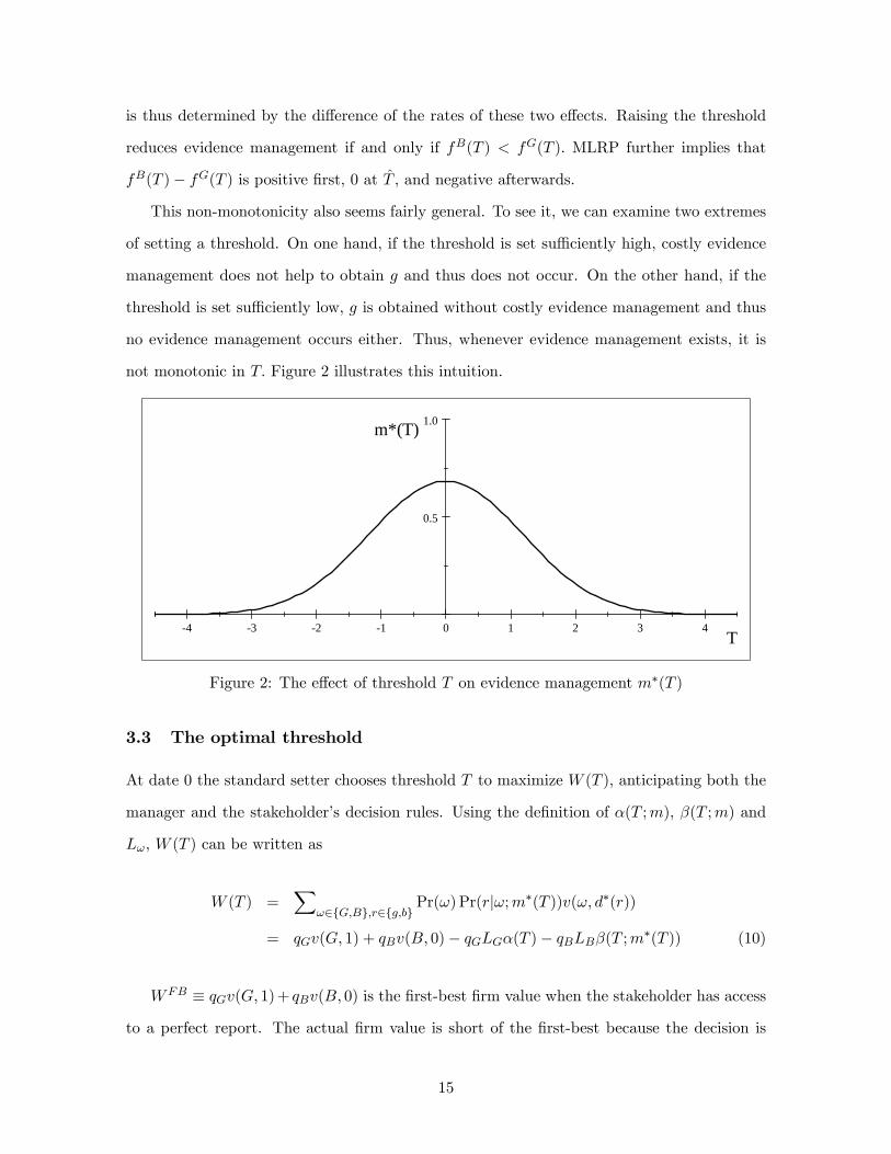
This non-monotonicity also seems fairly general. To see it, we can examine two extremes
of setting a threshold. On one hand, if the threshold is set suffi ciently high, costly evidence
management does not help to obtain g and thus does not occur. On the other hand, if the
threshold is set suffi ciently low, g is obtained without costly evidence management and thus
no evidence management occurs either. Thus, whenever evidence management exists, it is
not monotonic in T. Figure 2 illustrates this intuition.
4 3 2 1 0 1 2 3 4
0.5
1.0
T
m*(T)
Figure 2: The effect of threshold T on evidence management m∗(T )
3.3 The optimal threshold
At date 0 the standard setter chooses threshold T to maximize W (T ), anticipating both the
manager and the stakeholder’s decision rules. Using the definition of α(T ;m), β(T ;m) and
Lω, W (T ) can be written as
W (T ) =∑
ω∈{G,B},r∈{g,b}Pr(ω) Pr(r|ω;m∗(T ))v(ω, d∗(r))
= qGv(G, 1) + qBv(B, 0)− qGLGα(T )− qBLBβ(T ;m∗(T )) (10)
WFB ≡ qGv(G, 1) + qBv(B, 0) is the first-best firm value when the stakeholder has access
to a perfect report. The actual firm value is short of the first-best because the decision is
15

distorted by both the false alarm error, which costs qGLGα(T ), and the undue optimism error,
which costs qBLBβ(T ;m∗(T )). Had the standard setter been able to choose recognition errors
directly, she would set both α and β to be 0, thereby recognizing the transaction’s economic
substance "faithfully." However, the standard setter, unfortunately, cannot choose α and β
independently. Instead, she chooses threshold T to influence recognition errors indirectly.
Her threshold choice affects recognition errors through two different channels. The first is
an ex ante strategic effect: threshold T affects evidence management m that in turn affects
the distribution of evidence t and the recognition errors. The effect of threshold T on evidence
management m is ∂m∗(T )∂T , as captured in Lemma 2. The effect of evidence management on
recognition errors is ∂β(T ;m)∂m |m=m∗ > 0. Thus, the threshold’s strategic effect is captured by
∂β(T ;m)∂m
∂m∗(T )∂T |m=m∗ , whose sign is the same as that of ∂m∗(T )
∂T . This strategic effect relies
crucially on the fact that the standard setter’s choice of threshold T not only precedes the
manager’s choice of m but also is observed by the manager.
In addition to this strategic effect, the threshold also has an ex post statistical effect: for
any evidence t at date 2 (ex post), a higher threshold T reduces the undue optimism error at
the expense of increasing the false alarm error. That is, ∂β(T ;m∗)
∂T = −(m∗fG+(1−m∗)fB) < 0
and ∂α(T )∂T = fG > 0. This statistical effect is similar to that in the statistical benchmark
with the only difference that evidence t is now understood to be generated from f̃ω(t;m∗),
rather than fω(t).
To determine the optimal threshold T ∗, we differentiate the firm value W (T ) of equation
10 with respect to T. Assuming that T ∗ is interior, the first-order condition could be expressed
as
qGLG∂α(T )
∂T︸ ︷︷ ︸+
↑ false alarm
qBLB∂β(T ;m∗)
∂T︸ ︷︷ ︸↓undue optimism︸ ︷︷ ︸
T’s statistical effect
+ qBLB∂β(T ;m∗)
∂m∗∂m∗(T )
∂T︸ ︷︷ ︸affect EM︸ ︷︷ ︸
T’s strategic effect
= 0|m=m∗ = 0. (11)
The optimal threshold T ∗ is determined by balancing the threshold’s dual effects on
recognition errors weighted by their respective costs.5 The first two terms in equation 11
capture the threshold’s marginal effect on the firm value via the statistical effect. A higher
5With the general distribution functions, the firm value W is not necessarily concave in T. As a result,the first-order condition is necessary but may not be suffi cient for T ∗ to be the maximizer. However, allsubsequent results rely only on the first-order condition being necessary.
16

threshold affects recognition errors by ∂α(T )∂T and ∂β(T ;m∗(T ))
∂T , which in turn reduce the ex
ante firm value by qGLG and qBLB, respectively. The third term in equation 11 describes
the threshold’s marginal effect on the firm value via the strategic effect. The threshold
influences the manager’s evidence management decision by ∂m∗(T )∂T , evidence management
increases the undue optimism error by ∂β(T ;m)∂m |m=m∗ , and the undue optimism error reduces
the firm value by qBLB.
The model’s equilibrium is thus characterized by T ∗ satisfying equation 11, m∗(T ) deter-
mined by equation 8, and the d∗(r) described in equation 4. W (T ∗) and Assumption 3 now
can be expressed in terms of the model’s parameters.
3.4 The properties of the optimal threshold
With the equilibrium fully characterized, we are ready to answer the main research question
about the optimal level of P discussed in the Introduction. We first formally define P and
relate it to threshold T. Consider an accountant who has access to evidence t and understands
the manager’s choice m∗. Her belief of ω being good is p(t;m∗) ≡ Pr(G|t;m∗). Since p(t;m∗)
is monotonically increasing in t for any given m∗, the recognition standard T defined in
expression 2 can also be expressed by a constant P such that
r(t) = g if and only if p(t;m∗) ≥ P.
That is, the preferred treatment is granted if the probability that the state is good, condi-
tional on evidence and logic, exceeds P. T and P are thus two representations of thresholds.
To avoid confusion, we call P the probability threshold and T the evidence threshold.
The main advantage of working with P instead of T is that P is comparable across
different standards. T represents transaction characteristics that are multi-dimensional and
vary across different types of transactions. For example, transaction characteristics used
in a revenue recognition standard are very different from those employed in a contingency
standard. Thus, it is diffi cult to compare the evidence thresholds across the two standards. In
contrast, P is standardized as a probability and thus comparable across different standards.
For example, if revenue recognition requires that the probability of revenue being earned
17

exceeds 80% and contingent liability recognition requires that the probability of future loss
is 50%, then we might say that the former has a higher probability threshold.
A side benefit of the probability threshold representation is that it makes clear that
recognition thresholds exist even in the absence of bright-line cutoffs. Even a purely principle-
based recognition standard that does not contain evidence cutoffs still needs to specify a
probability threshold. For example, the legal burden of proof is "preponderance of evidence"
in most civil cases but "beyond reasonable doubt" in most criminal cases. While neither
might be associated with bright-line cutoffs, one probably would agree that they imply two
different probability thresholds.
Now we compare the probability thresholds with and without evidence management.
They can be calculated by using the Bayes rule, Lemma 1, and the first-order condition of
equation 11, respectively.
PBM ≡ p(TBM ) =qGf
G(TBM )
qGfG(TBM ) + qBfB(TBM )=
LBLB + LG
.
P ∗ ≡ p(T ∗;m∗) =qGf̃
G(T ∗;m∗)
qGf̃G(T ∗;m∗) + qB f̃B(T ∗;m∗)=
LBLB + LG + I(T ∗)
,
with I(T ∗) ≡qBLB
∂β(T ;m)∂m
qGfG∂m∗(T )
∂T|T=T ∗ . (12)
The optimal probability threshold in the benchmark PBM is determined by and only
by the recognition errors’relative costs to the stakeholder. The transaction’s details, such
as fω(t), are irrelevant (of course they still affect the evidence threshold). In contrast, the
optimal probability threshold with evidence management P ∗ has an additional determinant
I(T ∗) that is a function of the transaction’s details.
Proposition 1 P ∗ > PBM for T ∗ > T̂ , P ∗ = PBM for T ∗ = T̂ , and P ∗ < PBM for T ∗ < T̂ .
T̂ is the unique solution to fG(T ) = fB(T ).
Proposition 1 is the paper’s main result. It states that the presence of evidence manage-
ment does not necessarily result in a higher probability threshold, even though in the model
18
the manager always prefers a good report and evidence management always inflates evidence.
Its proof is immediate from inspecting the expression of I(T ∗). Since qBLBqGfG
∂β(T ;m)∂m |T=T ∗ > 0,
the sign of I∗(T ) is determined solely by ∂m∗(T )∂T |T=T ∗ , which is given in Lemma 2.
Consequently, the main intuition for Proposition 1 is derived from the intuition for Lemma
2. Recall that in Lemma 2 raising the threshold has a non-monotonic effect on evidence man-
agement. Since the threshold deviates from the statistical benchmark in order to discourage
evidence management, the direction of the deviation, or the sign of P ∗ − PBM , depends on
the direction of the threshold’s effect on evidence management. When T ∗ > T̂ , evidence
management is decreasing in the threshold and thus the optimal probability threshold P ∗
is raised above the statistical benchmark PBM . Similarly, when T ∗ < T̂ , evidence manage-
ment is increasing in the threshold and the optimal threshold designed to discourage evidence
management is lowered.
The exact location of T ∗ is determined implicitly by equation 11 and its closed-form
solutions are diffi cult to obtain. To illustrate Proposition 1, we present two examples, one with
P ∗ > PBM and the other P ∗ < PBM . Both use the following set of parameters: LG = LB = 1,
δB = 1.5, C(m) = m2
2 , c = 1, FG(t) = t for t ∈ [0, 1].
Example 1 FB(t) = t110 for t ∈ [0, 1]. qG = 0.25. Then T̂ = 0.08, T ∗ = 0.91, and P ∗ = 60%.
Example 2 FB(t) = t310 for t ∈ [0, 1]. qG = 0.6. Then T̂ = 0.18, T ∗ = 0.02, and P ∗ = 33%.
In both examples, PBM = 50% because LB = LG. Thus, in the absence of evidence
management, r = g is recognized as long as the probability of the state being good exceeds
50%, regardless of other aspects of the transaction. In Example 1, even though LB = LG,
the optimal probability threshold is 60%, higher than 50%. r = g is not recognized if the
probability of the state being good is higher than 50% but lower than 60%. Thus, the response
to inflatory evidence management is to raise the probability threshold, that is, to make it
more "conservative." For example, the probability threshold of revenue recognition is often
higher than 50%. While the excess might be caused by LB > LG, Proposition 1 provides an
alternative explanation.
In contrast, in Example 2, the optimal probability is 33%, even though LB = LG. The
reason is that T ∗ < T̂ . Raising the threshold in this region increases evidence management.
19

Thus, the optimal response to inflatory evidence management is to lower the probability
threshold, that is, to make it more "aggressive." For example, the probability threshold for
recognizing contingent obligations is usually interpreted as 75% (probable) in U.S. GAAP.
This means that the probability threshold for the preferred treatment (no recognition of lia-
bility) is 25%.While it might be explained as LB < LG, Proposition 1 provides an alternative
explanation.
P ∗ > PBM means that a higher likelihood of the good state is required for granting a
preferred treatment and thus might be interpreted as conservatism. Proposition 1 implies
that the optimal threshold response to inflatory evidence management is not necessarily con-
servative. Therefore, it highlights the different ways the instruments in the standard setter’s
toolkit work. Gao (2013a) shows that as far as the verification requirement is concerned, the
optimal response to inflatory evidence management is unambiguously conservative. That is,
favorable evidence is subject to more verification. Verification is costly but reduces recogni-
tion errors directly. Raising thresholds is free but affects recognition errors indirectly through
the statistical and strategic effects. The interaction between the two instruments and their
optimal combination are an interesting topic for future research.
Proposition 1 compares the ex ante optimal threshold with a statistical benchmark in the
absence of evidence management. Now we study another benchmark in which the standard
setter chooses an ex post effi cient threshold, that is, chooses a threshold to maximize the firm
value "on the basis of evidence and logic." This is consistent with a typical ex post notion
of providing maximum information to the stakeholder. Specifically, at date 2, the standard
setter observes evidence t and conjectures correctly that the manager has chosen m̃ at date 1.
While m̃ is endogenously chosen by the manager at date 1, it is a parameter of the evidence
generating process at date 2. Conditional on the transaction being type ω, the likelihood of
observing t is given by the density f̃ω(t; m̃). Thus, a threshold T would result in recognition
errors of α(T ) and β(T ; m̃) and the firm value of WFB − qGLGα(T ) − qBLBβ(T ; m̃). The
standard setter who maximizes the firm value at date 2 chooses the ex post effi cient threshold,
denoted as T̃ , according to the following first-order condition:
qGLG∂α(T )
∂T+ qBLB
∂β(T ; m̃)
∂T= 0. (13)
20

The ex post effi cient probability threshold P̃ ≡ p(T̃ ; m̃) can be derived from the Bayes
rule and the first-order condition of equation 13.
Proposition 2 1. P̃ = LBLB+LG
= PBM ;
2. When the threshold is set ex post, the firm value is lower and evidence management is
higher. That is, W (T̃ ) < W (T ∗) and m̃ > m∗.
The probability threshold implied by T̃ is the same as that in the statistical benchmark
without evidence management. Thus, the comparison of P̃ and P ∗ is straightforward from
Proposition 1. Even though the standard setter has rational expectations about evidence
management at date 2, she treats evidence management as given when setting the threshold.
Thus, the strategic effect is absent and the statistical effect alone determines the optimal
threshold. The rational expectations of evidence management modify the evidence generating
process from fω(t) to f̃ω(t;m), but do not affect the conceptual determination of the optimal
probability threshold. Therefore, what characterizes the strategic approach to threshold
design is the understanding that the threshold affects evidence management, not the rational
expectations of evidence management per se.
Part 2 of Proposition 1 summarizes the value of the standard setter’s ability to influ-
ence evidence management. Since recognition errors are costly to the stakeholder’s decision-
making in the model, the standard setter who chooses the threshold at date 0 considers both
the strategic and statistical effects of her choice. For the purpose of the stakeholder’s decision-
making at date 2, T̃ is the ex post effi cient threshold. For the purpose of curtailing evidence
management at date 1, T = t̄ or T = t completely eliminates evidence management. The ex
ante optimal threshold T ∗ balances these two effects and thus differs from either benchmark.
By moving away from T̃ , T ∗ reduces the ex post effi ciency of the stakeholder’s decision but at
the same time provides better control of the manager’s evidence management, which in turn
improves the ex ante effi ciency of the stakeholder’s decision. It is this commitment to ex post
ineffi cient use of information that discourages evidence management, which in turn improves
the ex ante informativeness of the report and the effi ciency of the stakeholder’s decision. In
contrast, when the threshold is chosen ex post, the threshold’s strategic effect is absent and
the standard setter loses one instrument to influence evidence management.
21
Finally, we conduct comparative statistics.
Proposition 3
1. The ex ante firm value (W ∗) is decreasing in δBc .
2. The optimal evidence threshold (T ∗) is not monotonic in δBc .
Part 1 of Proposition 3 is intuitive. The manager’s net incentive of evidence management
(i.e., δBc ) is unambiguously detrimental to the firm value because evidence management re-
duces the report’s equilibrium informativeness and distorts the stakeholder’s decision. Part
2 of Proposition 3 is also straightforward by now. An increase in δBc induces more evidence
management. Since evidence management decreases in the threshold if and only if T > T̂ ,
the optimal evidence threshold increases in δBc in this region to offset the increase in evidence
management. Thus, the non-monotonicity of the strategic effect lies behind the intuition.
4 Extensions
This section considers a number of extensions to the baseline model. In the baseline model,
a threshold affects recognition errors through both the classification of given evidence (the ex
post statistical effect) and the influence on evidence management that affects the distribution
of evidence (the ex ante strategic effect). These dual effects work differently, creating the
qualitative trade-off for the optimal threshold. In this section we check the robustness of
the presence of the dual effects to various assumptions. We pay particular attention to the
robustness of the non-monotonicity of the strategic effect because it has played an important
role in the main results.
4.1 Does disclosure of evidence dominate recognition?
It is necessary to assume the use of recognition in order to study threshold design. We have
justified recognition on empirical grounds that binary accounting treatment is prevalent in
accounting standards. Recognition always precedes measurement and is the first step to
incorporate a transaction into financial statements. Thus, studying threshold design for a
22
given recognition standard appears relevant to the understanding of financial reporting. On
the other hand, it is well understood that the discreteness in recognition induces evidence
management. Thus, one might be curious about what happens if the evidence is communi-
cated to the stakeholder through disclosure, rather than through recognition as assumed in
the baseline model. We show that compared with recognition, full disclosure of evidence in
the model lowers the firm value exactly because it induces more evidence management.
Proposition 4 Compared with the baseline model, the ex ante firm value is lower and evi-
dence management is higher if the accounting standard requires full disclosure of evidence to
the stakeholder.
The key proof strategy is to recognize that the stakeholder’s decision rule and the man-
ager’s evidence management in a disclosure equilibrium are payoff equivalent to those in a
recognition equilibrium with the threshold being set ex post. Disclosure of evidence t makes
the recognition report redundant because the latter is coarser. The stakeholder thus bases
the decision on evidence t to maximize the firm value. Since for any evidence management
a higher t still indicates a higher likelihood of the good state, the stakeholder’s decision rule
takes a cut-off form T0 such that d∗(t ≥ T0) = 1 and d∗(t < T0) = 0. T0 is the threshold that
maximizes the firm value on the basis of evidence t and the stakeholder’s understanding of
the manager’s influence on t. Therefore, T0 = T̃ , the ex post effi cient threshold defined in
equation 13. Full disclosure of evidence leads to the same decision rule for the stakeholder as
in recognition with an ex post effi cient threshold, which in turn implies that the manager’s
evidence management would be the same as m̃. Then Proposition 4 directly follows from
Proposition 2. The discussion following Proposition 2 suggests that it is the commitment to
ex post ineffi cient use of information that discourages evidence management and improves ex
ante effi ciency. Recognition, by coarsening the report, serves as such a commitment. In con-
trast, disclosure of evidence, by empowering the stakeholder, destroys the commitment. This
broad economic force behind Proposition 4, that controlling a manager’s ex ante incentive
requires the ineffi cient use of information ex post, is a recurring theme in the agency literature
(e.g., Arya, Glover, and Sivaramakrishnan (1997), Arya, Glover, and Sunder (1998)).
23

4.2 Endogenous conflict between the manager and the stakeholder
Facing the manager’s opportunistic evidence management, two intertwined responses can
arise. First, the standard setter can change the threshold. Second, the stakeholder can
adjust her use of the report. Both responses influence evidence management and they interact
with each other. By assuming exogenous δω, we have effectively isolated the stakeholder’s
response and focused exclusively on the threshold response. This differentiates our model
from previous studies. For example, if the manager’s benefit from a preferred report (δω)
were fixed, the threshold design would not affect the aggregate evidence management in Dye
(2002) (with the uniform distribution version). In this subsection, we explicitly model the
stakeholder’s decision in a capital market setting to provide a "micro-foundation" for δω. The
stakeholder’s response adds an indirect channel through which the threshold affects evidence
management, but the direct channel in the baseline model is preserved.
The timeline is the same as before. The manager is interpreted as an entrepreneur with a
project that requires investmentK at date 2.Without the investment the project is worthless.
With the investment it pays out either Y (success) or 0 (failure) at date 3. Its success
probability is γω, which depends on the firm’s financial condition ω (the state of nature).
At date 2 after issuing report r the entrepreneur sells the project to investors (the stake-
holder) for life cycle reasons at an endogenously determined price A(r). After the purchase
investors decide whether to invest K (d = 1) or not (d = 0). Their payoff related to this
decision is v(ω, d) = (γωY −K)d and we have LG ≡ v(G, 1)− v(G, 0) = γGY −K > 0, and
LB ≡ v(B, 0)− v(B, 1) = K − γBY > 0. Hence, Assumption 1 is satisfied.
Denotem∗∗ as the equilibrium evidence management. Similar to Assumption 3, we assume
that the equilibrium report is informative enough to influence the investment decision, that is,∑ω∈{G,B} Pr(ω|g;m∗∗)γωY > K >
∑ω∈{G,B} Pr(ω|b;m∗∗)γωY. Thus, the investors’decision
rule is d∗(g) = 1 and d∗(b) = 0.
A(r) is a transfer between the entrepreneur and investors. The entrepreneur’s payoff is
u(ω, d∗(r)) = A(r). As standard, we assume that investors face a competitive capital market,
24

expect zero net surplus, and price the project accordingly. Then A(r) can be determined as
A(g) =∑
ω∈{G,B}Pr(ω|g;m∗∗)γωY −K,
A(b) = 0.
Anticipating A(r), the entrepreneur prefers r = g to r = b and δB(T ;m∗∗) ≡ A(g)−A(b) >
0. Hence, Assumption 2.
The rest setup is the same as in the baseline model. This new setting’s key difference from
the baseline model is that δB(T ;m∗∗) is an endogenous function of the threshold and evidence
management. To see its impact, we first derive the first-order condition of the entrepreneur’s
choice of evidence management at date 1:
qB(FB(T )− FG(T ))δB(T ;m∗∗) = cC ′(m∗∗(T )). (14)
Differentiating it with respect to T, we have
qB(fB − fG)δB︸ ︷︷ ︸direct channel
+qB(FB − FG)(∂δB(T ;m∗∗)
∂T+∂δB(T ;m)
∂m
∂m∗∗(T )
∂T|m=m∗∗)︸ ︷︷ ︸
indirect channel
= cC ′′∂m∗∗(T )
∂T.
(15)
The comparison between equation 9 and 15 reveals that endogenizing δB(T ;m∗∗) adds
an indirect channel for the threshold to affect evidence management. In the baseline model,
threshold T affects only the probability of receiving a preferred treatment (qB(FB(T ) −
FG(T )) in equation 14). An endogenous δB(T ;m∗∗) means that threshold T now also af-
fects the benefit of receiving a preferred treatment (δB(T ;m∗∗) in equation 14) when in-
vestors adjust the interpretation and use of the report in their pricing decision. This indi-
rect channel consists of two component. First, δB(T ;m)∂T > 0.6 Fixing evidence management,
a higher threshold increases a good report’s informativeness and thus its price. Second,
δB(T ;m)∂m |m=m∗∗ < 0. Fixing the threshold higher evidence management reduces a good re-
port’s informativeness and thus its price. The total effect of the indirect channel is thus
6The proof is by straightforward derivatives and utilizes the result that MLRP implies monotone hazard
ratio, that is, fB(T )
1−FB(T )> fG(T )
1−FG(T ).
25

captured by dδB(T ;m∗∗(T ))
dT = ∂δB(T ;m∗∗)
∂T + ∂δB∂m∗∗
∂m∗∗(T )∂T .
The net effect of the threshold on evidence management in equilibrium, ∂m∗∗(T )∂T , could be
rewritten as
∂m∗∗(T )
∂T(cC ′′−qB(FB−FG)
∂δB(T ;m)
∂m|m=m∗∗) = qBδB(fB(T )−fG(T ))+
∂δB(T ;m∗∗)
∂TqB(FB−FG)
(16)
While a closed-form solution of ∂m∗∗(T )∂T requires specifying the evidence distributions, its
sign can be discussed with the general distributions. First, ∂m∗∗(T )∂T 6= 0 in general. Second,
the sign of ∂m∗∗(T )∂T can be dominated by qBδB(fB(T ) − fG(T )) because (cC ′′ − qB(FB −
FG)∂δB(T ;m)∂m |m=m∗∗) > 0 and ∂δB(T ;m∗∗)
∂T > 0. Therefore, the threshold’s strategic effect is
still present and its non-monotonicity can be preserved.
Since A(r) is a transfer, its endogenization does not affect the standard setter’s objective
function W (T ). The new first-order condition for the ex ante optimal threshold T ∗∗ has the
same form as in equation 11 except that ∂m∗∗(T )∂T is more complicated with the indirect channel
discussed above. As a result, the qualitative characterization of the optimal threshold in the
baseline model in Section 3.4 is intact.
We have highlighted that we exploit a different channel through which threshold design
interacts with evidence management and recognition errors. In Dye (2002), a threshold affects
investors’rational interpretations of the report and their pricing, which in turn affects the
manager’s benefit of receiving a preferred report and thus his evidence management. This
channel is isolated in the baseline model of this paper by the assumption of an exogenous
conflict of interest between the stakeholder and the manager. Instead, this paper focuses on
a different channel. The threshold affects the classification of evidence, which in turn changes
the manager’s probability of receiving a preferred report and thus his evidence management.
This channel makes it possible to study this paper’s main research question of comparing
a strategic approach to threshold design with its statistical counterpart in a setting with
minimum departure from the statistical literature. It generates the central trade-off of the
threshold’s strategic and statistical effects and the main result that the optimal threshold is
not monotonic in evidence management. In other words, this paper differs from Dye (2002)
26

in both their main results and the economic forces behind the results.
4.3 Different technologies of evidence management
In the baseline model evidence management improves the distribution of evidence only in
the bad state. As a result, evidence management is unambiguously detrimental to the stake-
holder’s decision-making. Despite the desirability of reducing evidence management, the
threshold’s optimal response is not monotone because of its non-monotone effect on evidence
management. In this subsection we consider a more general technology of evidence manage-
ment that improves the evidence distributions in both states. As a result, it can be optimal to
encourage evidence management. This ambiguity of the desirability of evidence management
adds an orthogonal reason that the threshold’s optimal response to evidence management is
not monotone.
Specifically, we modify f̃ω(t;m) as mfMω(t)+(1−m)fω(t) with fMω (t)fω(t) strictly increasing
in t. The baseline model is a special case of fMω = fG. The manager’s first-order condition
for m becomes ∑ω∈{G,B}
qω[Fω(T )− FMω(T )]δω = cC ′(m∗(T )).
∂m∗(T )
∂T=∑
ω∈{G,B}qωδωcC ′′
(fω(T )− fMω(T )).
Again the non-monotonic strategic effect is preserved because ∂m∗(T )∂T is not monotonic in
T . Working through the first-order condition of the optimal threshold, we can characterize
the optimal probability threshold as
P ∗ =LB
LB + LG + I(T ∗)
with I(T ∗) ≡qBLB
∂β(T ;m)∂m + qGLG
∂α(T ;m)∂m
qGf̃G∂m∗(T )
∂T|T=T ∗ . (17)
The optimal probability threshold is the same as that in the baseline model except that
I(T ∗) becomes more complicated in comparison with equation 12. The major difference
is that the numerator has a new component qGLG∂α(T ;m)∂m < 0. That is, evidence manage-
27

ment can reduce the false alarm error. Since qBLB∂β(T ;m)∂m > 0, the first term in I(T ∗),
qBLB∂β(T ;m)∂m
+qGLG∂α(T ;m)∂m
qGf̃G, can go either direction, depending on the relative importance of
m on the evidence distributions in two states. Since evidence management increases the
undue optimism error and reduces the false alarm error, whether evidence management is
detrimental to the stakeholder’s decision depends on the relative importance of each effect.
As a result, the sign of I(T ∗) is determined not only by ∂m∗(T )∂T (as in the baseline model)
but also byqBLB
∂β(T ;m)∂m
+qGLG∂α(T ;m)∂m
qGf̃G. The latter determinant adds one more reason that the
optimal threshold response is non-monotonic, but it is orthogonal to the reason studied in
the baseline model.
We also consider a different technology of evidence management. In the baseline model,
the evidence management choice is continuous. We consider another modeling device of
evidence management in which the manager either engage in evidence management or not.
For example, to improve the chance that a lease contract qualifies for operating lease, the
manager has to decide whether to hire a consulting firm to structure the lease contract or not.
Specifically, the manager’s private cost of evidence management is c > 0, with differentiable
density and cumulative distribution functions h(c) and H(c), respectively. We also consider
only "bad" evidence management. If the manager engages in evidence management, t is
drawn from fG(t) instead of fω(t). The manager decides whether to engage in evidence
management after observing his cost c but before observing the state.
This new setting preserves the threshold’s strategic effect on recognition errors. For any
given T, the manager engages in evidence management if and only if c ≤ c∗(T ), with c∗(T )
being determined by
qB[FB(T )− FG(T )]δB = c∗(T ).
Differentiating it with respective to T, we have
∂c∗(T )
∂T= qB[fB(T )− fG(T )]δB
Thus, the threshold’s effect on evidence management is qualitatively the same as in the
baseline model. As a result, the main results in the baseline model can be replicated with
28
little modification.
4.4 Different timing of evidence management
In the baseline model, the manager makes the choice without observing ω or t. In this sub-
section we consider the case when the manager chooses evidence management after observing
initial evidence t′, as in Dye (2002) and Laux and Stocken (2017).
If t′ > T, evidence management is not necessary and the manager reports t = t′. If
t′ < T, the benefit of inflating t′ to T depends on the realization of t′. For simplicity, we
assume that δB = δG = δ, as in the case of the capital market setting in Subsection 4.2. We
also assume that it costs the manager a unit cost of c to add T − t′ to the initial evidence t′.
For any threshold T, define t0(T ) as the solution δ = (T − t0(T ))c. The manager’s evidence
management decision m is a function of t′ :
m(t′) =
T − t′ for t′ ∈ (t0(T ), T )
0 otherwise.
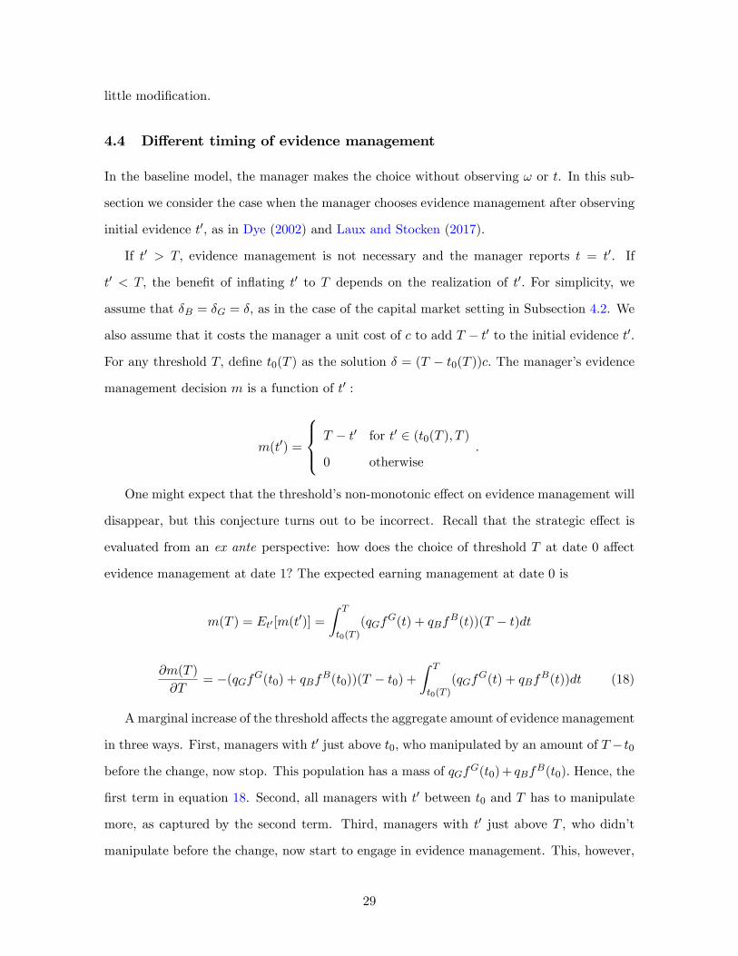
One might expect that the threshold’s non-monotonic effect on evidence management will
disappear, but this conjecture turns out to be incorrect. Recall that the strategic effect is
evaluated from an ex ante perspective: how does the choice of threshold T at date 0 affect
evidence management at date 1? The expected earning management at date 0 is
m(T ) = Et′ [m(t′)] =
∫ T
t0(T )(qGf
G(t) + qBfB(t))(T − t)dt
∂m(T )
∂T= −(qGf
G(t0) + qBfB(t0))(T − t0) +
∫ T
t0(T )(qGf
G(t) + qBfB(t))dt (18)
A marginal increase of the threshold affects the aggregate amount of evidence management
in three ways. First, managers with t′ just above t0, who manipulated by an amount of T − t0
before the change, now stop. This population has a mass of qGfG(t0) + qBfB(t0). Hence, the
first term in equation 18. Second, all managers with t′ between t0 and T has to manipulate
more, as captured by the second term. Third, managers with t′ just above T , who didn’t
manipulate before the change, now start to engage in evidence management. This, however,
29

does not affect the total amount of evidence management because each manipulates only an
infinitesimal amount. This explains equation 18. In general, ∂m(T )∂T 6= 0 and can be either
positive or negative, depending on the shapes of fω and Fω. Therefore, the threshold’s non-
monotonic strategic effect is still preserved, and so is the qualitative trade-off of threshold
design in the baseline model.
5 Empirical implications
The paper has three major empirical implications. First, the mere difference between P ∗
and PBM reveals an additional determinant of the optimal threshold. In the absence of ev-
idence management, the optimal threshold PBM = LBLB+LG
is determined solely by costs of
recognition errors for the stakeholder. In particular, the transaction’s details are irrelevant.
In contrast, since P ∗ has an additional determinant I(T ∗), it varies not only with the stake-
holder’s decision problem but also with the transaction-specific features, such as fω(t) and
c. fω(t) is the link between the transaction’s economic substance and evidence. It may be
interpreted as the relevance of a transaction characteristic. c captures the link’s vulnerability
to the manager’s influence and may be interpreted as the reliability of a transaction charac-
teristic. Since this additional determinant varies across transactions, it seems more suitable
for explaining the cross sectional differences in observed thresholds across transactions, in-
dustries, jurisdictions, and over time.
For example, the probability threshold P implied in most revenue recognition standards
seems to be higher than 50%. One common explanation for the excess is that LB > LG, that
is, early recognition is more costly than delayed recognition. Proposition 1 predicts that even
after controlling for LB and LG, the excess can still exist and it varies with both the relevance
and reliability of transaction characteristics used in the standards. For another example,
according to the model, one reason for the different probability thresholds of the contingent
liabilities under IFRS and the US GAAP can be that preparers’ ability and incentive to
structure transactions to influence accounting evidence differ in respective jurisdictions. As
standard setters are contemplating on revising revenue recognition standards and converging
U.S. GAAP with IFRS, our model could help shed some light on these complex issues.
30

Second, the ex ante optimal threshold, which maximizes the report’s ex ante value for
decision making (before the evidence is generated), differs from the ex post effi cient threshold,
which maximizes the report’s ex post value (after the evidence is generated). Since both
approaches maximize the report’s information for the stakeholder’s decision making, standard
setters can defend themselves better by making it clear which approach they intend to pursue.
If the ex post approach is chosen, then standards should be evaluated according to Proposition
2. If the ex ante approach is intended, then Proposition 1 should be the basis for the
evaluation. In the latter case, Proposition 2 predicts that the ex ante optimal threshold is
vulnerable to the criticism that it does not make the best use of evidence available ex post.
Accordingly, some safeguards against such ex post pressure, such as the independence of
standard setters, are desirable.
Finally, the model reveals the richness of accounting standard setting. The model suggests
that one key comparative advantage of standard setters is to document a transaction’s details,
which seems to be at the core of accounting standard setting process in practice. Moreover,
these details evolve over time and thus standards need to be revised continually.
The tests of all these empirical predictions call for data about the costs of recognition
errors (Lω), the empirical distributions of a transaction’s economic substance and its charac-
teristics (fω(t)), and managers’incentive and ability to influence these distributions (δω and
c).
6 Discussions and conclusions
This paper studies the optimal design of recognition thresholds in accounting standards.
When a threshold choice induces managers to influence the very accounting evidence the
threshold classifies, the threshold choice has dual effects on recognition errors. On one hand,
after the evidence is presented, a higher threshold reduces the undue optimism error at
the expense of raising the false alarm error. This is the familiar statistical effect. On the
other hand, before the evidence is produced, the threshold influences managers’ evidence
management, which in turn affects the distribution of accounting evidence and the ex post
recognition errors. This is the strategic effect. The statistical and strategic effects differ from
31

each other both quantitatively and qualitatively. As a result, the optimal threshold under
the strategic approach, which balances the dual effects, behaves differently from that under
the statistical approach. In particular, in the presence of inflatory evidence management the
optimal threshold can either be higher or lower than its statistical benchmark. The insights
from the statistical approach provide limited and misleading guidance for optimal threshold
design.
To focus on recognition threshold design, we have taken the use of recognition standards
as given. While this choice might be justified on empirical grounds, the problem of the
inherent discontinuity in recognition, the "all-or-nothing" feature, is well-known and various
alternatives have been proposed to mitigate it. One alternative is to use a more continuous
recognition or measurement approach. Another is to reduce the reliance on bright-line rules
and move towards a more principle-based system. Investigating the general rationale for
recognition by comparing it with these alternatives is a promising avenue for future research.
Liang (2001) surveys the litearture on accounting recognition.
To mitigate the concern that the main results are an artifact of imposing suboptimal
binary recognition in the model, we have restricted the stakeholder’s decision to be binary.
This assumption assures that binary recognition is indeed optimal in the model. In addition,
the binary decision assumption also fits the model well with the vast statistical literature on
hypothesis testing and, as such, facilitates the model’s contrast with its statistical benchmark.
Nonetheless, the binary decision is a restriction on the model. As we understand more about
the rationale for binary recognition, we should also extend the threshold design problem to
a more general decision making setting.
A related limitation of this paper is that the standard setter in the model serves as a
convenient stand-in for a rule designer. The same results can be obtained if the manager and
the stakeholder can design the rule and commit to it. Thus, to interpret our model in the
context of mandatory financial reporting, we have to assume that reporting regulation serves
as a low-cost commitment device, an argument elaborated by Mahoney (1995) and Rock
(2001). The economic justifications for mandatory financial reporting are still hotly debated
(see Leuz and Wysocki (2007) for a survey of the debate). Apparently, an alternative view
about the rationale is likely to have different implications for the optimal rule design.
32

7 Appendix
Proof. of Proposition 2: Part 1 is derived directly from the definition of P̃ and the first-order
condition of equation 13. To prove Part 2, note that T̃ is feasible for the standard setter at
date 0 but not chosen. Therefore, we have ρ ≡ W (T ∗;m∗) − W (T̃ ; m̃) > 0. m∗ < m̃ is
proved by contradiction. Suppose m∗ ≥ m̃. Since ∂W (T ;m)∂m = −qBLB(FB(T ) − FG(T )) < 0
for any T ∈ (t, t̄), we have W (T ∗;m∗)−W (T ∗; m̃) ≤ 0. Moreover, by definition T̃ maximizes
W (T̃ ; m̃) for given m̃. Thus, W (T ∗; m̃) −W (T̃ ; m̃) < 0. Combining the two, we have ρ =
(W (T ∗;m∗) −W (T ∗; m̃)) + (W (T ∗; m̃) −W (T̃ ; m̃)) = W (T ∗;m∗) −W (T̃ ; m̃) < 0. Hence a
contradiction. Thus, m∗ < m̃.
Proof. of Proposition 3: Part 1 is proved by the envelope theorem and Lemma 2. To prove
Part 2, we apply the implicit function theorem to equation 11: dT∗
dc = −∂2W∂T∂c∂2W∂T2
. Since T ∗ is the
maximizer, ∂2W∂T 2 < 0. Thus, dT
∗
dc has the same sign as ∂2W∂T∂c . Differentiating equation 11 with
respect to c and simplifying the terms, we have
∂2W
∂T∂c= −qBLB(fB − fG)
∂m∗
∂c− qBLB(FB − FG)
∂2m∗
∂T∂c
= qBLB(FB − FG)
c(1 +
(C ′′)2 − C ′C ′′′(C ′′)2
)∂m∗
∂T
Therefore, the sign for dT ∗
dc is the same as ∂m∗
∂T . The case for δB can be proved similarly.
References
Arya, A., J. Glover, and K. Sivaramakrishnan, 1997, The interaction between decision andcontrol problems and the value of information, The Accounting Review 72, 561—574.
Arya, A., J. Glover, and S. Sunder, 1998, Earnings management and the revelation principle,Review of Accounting Studies 3, 7—34.
Bertomeu, J., and E. Cheynel, 2013, Toward a positive theory of disclosure regulation: Insearch of institutional foundations, The Accounting Review 88, 789—824.
Bertomeu, J., and R.P. Magee, 2011, From low-quality reporting to financial crises: Politicsof disclosure regulation along the economic cycle, Journal of Accounting and Economics52, 209—227.
Beyer, A., D.A. Cohen, T.Z. Lys, and B.R. Walther, 2010, The financial reporting environ-ment: Review of the recent literature, Journal of Accounting and Economics 50, 296—343.
33

Chen, Q, T.R. Lewis, K. Schipper, and Y. Zhang, 2017, Uniform versus discretionary regimesin reporting information with unverifiable precision and a coordination role, Journal ofAccounting Research 55, 153—196.
Dechow, P.M., and C. Shakespear, 2009, Do managers time securitization transactions toobtain accounting benefits?, The Accounting Review 84, 99—132.
Dye, R., 2002, Classifications manipulation and Nash accounting standards, Journal of Ac-counting Research 40, 1125—1162.
Engel, E., M. Erickson, and E.L. Maydew, 1999, Debt-equity hybrid securities, Journal ofAccounting Research 37, 249—274.
Ewert, R., and A. Wagenhofer, 2012, Earnings management, conservatism, and earningsquality, Foundations and Trends R© in Accounting 6, 65—186.
Fan, Q., and X.J. Zhang, 2012, Accounting conservatism, aggregation, and information qual-ity, Contemporary Accounting Research 29, 38—56.
FASB, 2010, Statement of Financial Accounting Concepts No. 8: Conceptual Framework forFinancial Reporting, Financial Accounting Standards Board of the Financial AccountingFoundation.
Gao, P., 2013a, A measurement approach to conservatism and earnings management, Journalof Accounting and Economics 55, 251—268.
, 2013b, A two-step representation of accounting measurement, Accounting Horizons27, 861—866.
Holmstrom, B., 1999, Managerial incentive problems: A dynamic perspective, The Review ofEconomic Studies 66, 169—182.
Imhoff, E., and J.K. Thomas, 1988, Economic consequences of accounting standards: Thelease disclosure rule change, Journal of Accounting and Economics 10, 277—310.
Kaplow, L., 2011, On the optimal burden of proof, Journal of Political Economy 119, 1104—1140.
Laux, V., and P. Stocken, 2017, Accounting standards, regulatory enforcement, and invest-ment decisions, working paper, University of Texas at Austin.
Leuz, C., and P.D. Wysocki, 2007, Economic consequences of financial reporting and disclo-sure regulation: What have we learned?, Chicago Booth working paper.
Liang, P.J., 2001, Recognition: An information content perspective, Accounting Horizons 15,223—242.
Lys, T.Z., and L. Vincent, 1995, An analysis of value destruction in AT&T’s acquisition ofNCR, Journal of Financial Economics 39, 353—378.
Magee, R.P., 2006, Reasonably certain estimates, recognition, and communication of uncer-tainty, working paper, Northwestern University.
Mahoney, P.G., 1995, Mandatory disclosure as a solution to agency problems, The Universityof Chicago Law Review 62, 1047—1112.
Milgrom, P.R., 1981, Good news and bad news: representation theorems and applications,The Bell Journal of Economics 12, 380—391.
Mittendorf, B., 2010, The role of audit thresholds in the misreporting of private information,Review of Accounting Studies 15, 243—263.
34

Neyman, J., and E.S. Pearson, 1933, On the problem of the most effi cient tests of statisticalhypotheses, Philosophical Transactions of the Royal Society A 231, 289—337.
Rock, E., 2001, Securities regulation as lobster trap: A credible commitment theory of manda-tory disclosure, Cardozo Law Review 23, 675—704.
SEC, 2005, Report and recommendations pursuant to section 401(c) of the Sarbanes-OxleyAct of 2002 on arrangements with off-balance sheet implications, special purpose entities,and transparency of filings by issuers, SEC Staff Report.
Shleifer, A., and D. Wolfenzon, 2002, Investor protection and equity markets, Journal ofFinancial Economics 66, 3—27.
Spence, M., 1973, Job market signaling, The Quarterly Journal of Economics 87, 355—374.
Stein, J.C., 1989, Effi cient capital markets, ineffi cient firms: A model of myopic corporatebehavior, The Quarterly Journal of Economics 104, 655—669.
Stocken, P., 2013, Strategic accounting disclosure, Foundations and Trends R© in Accounting7, 197—291.
35