Ohd

Ja

b

c

d

a

ARR1AA

KSLA

1

&itvowat

tgtuLsd

ara

0h

Computers and Chemical Engineering 62 (2014) 211– 224

Contents lists available at ScienceDirect

Computers and Chemical Engineering

jo u r n al homep age: www.elsev ier .com/ locate /compchemeng

ptimal supply chain design and management over a multi-periodorizon under demand uncertainty. Part II: A Lagrangeanecomposition algorithm

iang Yonghenga, Maria Analia Rodriguezb, Iiro Harjunkoskic, Ignacio E. Grossmannd

Institute of Process Control Eng., Department of Automation, Tsinghua University, Beijing 100084, PR ChinaINGAR (CONICET-UTN), Avellaneda 3657, Santa Fe 3000, ArgentinaABB AG, Corporate Research Germany, Wallstadter Straße 59, 68526 Ladenburg, GermanyCenter for Advanced Process Decision-Making, Department of Chemical Engineering, Carnegie Mellon University, Pittsburgh, PA 15213, USA

r t i c l e i n f o

rticle history:eceived 6 June 2013eceived in revised form7 November 2013ccepted 22 November 2013vailable online 7 December 2013

eywords:upply chainagrangean decompositiondaptive piecewise linearization

a b s t r a c t

In Part I (Rodriguez, Vecchietti, Harjunkoski, & Grossmann, 2013), we proposed an optimization model toredesign the supply chain of spare parts industry under demand uncertainty from strategic and tacticalperspectives in a planning horizon consisting of multiple time periods. To address large scale indus-trial problems, a Lagrangean scheme is proposed to decompose the MINLP of Part I according to thewarehouses. The subproblems are first approximated by an adaptive piece-wise linearization schemethat provides lower bounds, and the MILP is further relaxed to an LP to improve solution efficiencywhile providing a valid lower bound. An initialization scheme is designed to obtain good initial Lagrangemultipliers, which are scaled to accelerate the convergence. To obtain feasible solutions, an adaptivelinearization scheme is also introduced. The results from an illustrative problem and two real worldindustrial problems show that the method can obtain optimal or near optimal solutions in modestcomputational times.

© 2013 Elsevier Ltd. All rights reserved.

. Introduction

In the spare parts industry, or more specifically the electric motor industry as was illustrated in part 1 (Rodriguez, Vecchietti, Harjunkoski, Grossmann, 2013), there are some key issues that strongly influence the cost of the supply chain. One is that a low-level inventory is

mportant (bound capital). Moreover, it is critical that a spare motor can be obtained as soon as possible since the motor is a key part ofhe customer plant. Tens or hundreds of different types of motors are required by the customers. Also, the criticality of a given unit can beery different. If the time requirement is very tight, it might be necessary to have some motors in stock at the customer sites. The mainbjective of the model is to optimally redesign supply chain to meet the demand with minimal costs involving decisions on where to placearehouses, which installed warehouses should be expanded or shutdown, as well as deciding the stock capacities, safety stocks required,

nd how to connect the different echelons of the supply chain in order to satisfy uncertain demand of motors. Due to the above features,he problem corresponds to a large scale MINLP problem that is very hard to solve.

Lagrangean decomposition has been successfully applied to large-scale mathematical programming problems (Wang, 2003). Accordingo the problem structure, temporal and spatial decomposition can be adopted (Terrazas-Moreno, Trotter, & Grossmann, 2011). The sub-radient optimization is a popular method for updating the multipliers in Lagrangean decomposition (Baker and Sheasby, 1999), althoughhe convergence of the multipliers is the main challenge. Other contributions include methods for accelerating convergence through these of subgradients (Baker and Sheasby, 1999; Fumero, 2001) and other strategies (Mouret, Grossmann, & Pestiaux, 2011; Buil, Piera, &uh, 2012). In Terrazas-Moreno et al. (2011), an economic interpretation of the multipliers is given, which can benefit from the problemtructure to accelerate the convergence. Considering that the dual problem is a high-dimensional nonlinear problem, the shape of itsomain and contours is a key to accelerate the convergence, and the interpretation from an economic view may be helpful.

This paper is organized as follows. In Section 2, the model from Part I is reformulated. In Section 3, a decomposition scheme is proposed,nd the methods to solve the subproblems, initialize and update the multipliers, and design of the feasibility problem are discussed. The

esults from an illustrative example and two real world industrial problems are shown and discussed in Section 4. Finally, some conclusionsre drawn in Section 5.

098-1354/$ – see front matter © 2013 Elsevier Ltd. All rights reserved.ttp://dx.doi.org/10.1016/j.compchemeng.2013.11.014

212 J. Yongheng et al. / Computers and Chemical Engineering 62 (2014) 211– 224

Nomenclature

Indicesc criticality levels of motorsi factoriesj warehousesk end customersp standard unitss special unitst time periods

SetsCTks customers k that allow used repaired units to satisfy their demand of unitsJF subset of warehouses j that are already installed (fixed) at the beginning of the horizon planningKSCksc customers k that order special units s of criticality cKTks customers k that order tailor made units sPSps special units s belonging to standard unit pSC subset of warehouses j that can be also considered as repair workshops

Binary variablesuikst if factory i produces and delivers tailor made unit s to end customer k in period tvjkst if repair workshop j repairs special units s from customer k in period twit if factory i is installed in period twe

itif warehouse j is expanded in period t

wuit

if factory i is uninstalled (eliminated) in period txijpt if factory i produces and delivers standard units p to warehouse j in period tyjt if warehouse j is installed in period tye

jtif warehouse j is expanded in period t

yujt

if warehouse j is uninstalled (eliminated) in period tzjkt if warehouse j delivers units to customer k in period tˇI auxiliary variable for linearization of subproblems

Positive variableslksct net lead time of customer k for special unit s of criticality c in period tl′jksct

net lead time of customer k if special unit s of criticality c is provided by warehouse j in period tmksct net lead time of customer k for tailor made unit s of criticality c in period tm′

jksctnet lead time of customer k if tailor made unit s of criticality c is provided by warehouse j in period t

TIt the total investment cost in period tTIwtj the total investment costin new warehouse j in period tTOFt the total operational fixed cost in period tTOFwtj the total operational fixed cost in warehouse j in period tTEt the total investment expansion cost in period tTEwtj the total investment expansion cost in warehouse j in period tTUt the total shutdown cost in period tTUwtj the total shutdown cost in warehouse j in period tTOVt the total variable cost in period tTOVwtj the total variable cost in warehouse j in period tTPVt the total variable cost in factories for the motors transported in period tTPVwtj the total variable cost in factories for the motors transported to warehouse j in period tTRt the repair cost in period tTRwtj the repair cost in warehouse j in period tTTFt the transportation cost from factories to warehouses and customer sites in period tTTFwtj the transportation cost from factories to warehouse j in period tTTFctT the transportation cost from factories to customer sites in period tTTWt the transportation cost in period tTTWwtj the transportation cost from warehouse j in period tTPCt the mean inventory cost at customer sites for the special motors from warehouse and tailor made motors in period tTPCwtj the mean inventory cost at customer sites for the special motors from warehouse j in period tTPCctT the mean inventory cost at customer sites for the special motors from tailor made motors in period tTSSt the summation of the safety stock cost in period tTSSwtj the summation of the safety stock cost at warehouse j and customer sites for the special motors from warehouse j in period

t

J. Yongheng et al. / Computers and Chemical Engineering 62 (2014) 211– 224 213

TSSctT the safety stock cost at customer sites for tailor made motors in period tTBTt the lost sales stock cost for special motors in period tTBTwtj the lost sales stock cost for special motors from warehouse j in period t�zkt; �vskt; �c the positive Lagrange multipliersaI, a′

I�1, �2 auxiliary variables for linearization of subproblems�new

ijkptamount of demand of standard units p from customer k satisfied with new units from factory i and warehouse j

�usedjkst

amount of demand of special units s from customer k satisfied with used units from repair workshop j�new

ikstamount of demand of tailor made units p from customer k satisfied with new units from factory i

�usedjkst

amount of demand of tailor made units s from customer k satisfied with used units from repair workshop j

Variablesg = (gzT

kt, gvT

skt, gmuctT

kpt, gtolT

ks, gcT )

Tthe subgradients of the Lagrangean function

x the general independent variablexp the solution of the previous iteration for linearization of feasibility problemxt the temporal variables for linearization of subproblemsy the general dependent variableL the Lagrangean functionLj the part for warehouse j of the Lagrangean functionLr the remaining part of the Lagrangean function excluding Lj�muctkpt; �tolkst the Lagrange multipliers

Parametersa the scalar for linearization of feasibility problemb1ks unit annual lost sales cost for special unit s at customer kc1ij unit transportation cost from factory i to warehouse jc2jk unit transportation cost from warehouse j to customer kc3ik unit transportation cost from factory i to customer kt2jkp order processing time of customer k for standard unit p if it is served by warehouse j, including material handling time in

k, transportation time from warehouse j to k, and inventory review period in the customer site˛p production factor rate for standard unit p˛z , ˛v, ˛t the scalars for subgradient scaling�ksct mean demand of special units s of criticality c from customer k in period t�ksct demand standard deviation of special units s of criticality c from customer k in period t

L U

2

cmfi

i

w

w

w

w

x , x the lower and upper bounds of xx days in the year

. The supply chain model reformulation

In order to design the decomposition algorithm, we reformulate the model from Part I to aggregate the terms in the objective andonstraints according to the warehouses for which we consider potential selection, capacity expansion and shutdowns. In the reformulatedodel, we assume for simplicity that no factory expansion and shutdown are considered. That is, all the necessary factories are given with

xed capacities at the beginning of time horizon for the design of the supply chain.Firstly, the cost terms (Eqs. (54), (56), (58), (60), (62)–(70) from Part I) are disaggregated in the objective function (Eq. (72) from Part I)

n terms of the warehouses j, as follows.

TIt =∑

jTIwtj ∀ t (1)

here TIwtj denotes the total investment cost in new warehouse j in period t.

TOFt =∑

jTOFwtj ∀ t (2)

here TOFwtj denotes the total operational fixed cost in warehouse j in period t.

TEt =∑

jTEwtj ∀ t (3)

here TEwtj denotes the total investment expansion cost in warehouse j in period t.

TUt =∑

jTUwtj ∀ t, ∀ t (4)

here TUwtj denotes the total shutdown cost in warehouse j in period t.

TOVt =∑

jTOVwtj ∀ t (5)

2

wf

w

w

wi

wi

a

c

3

3

fe(

14 J. Yongheng et al. / Computers and Chemical Engineering 62 (2014) 211– 224

where TOVtj denotes the total variable cost in warehouse j in period t.

TPVt =∑

jTPVwtj ∀ t (6)

where TPVwtj denotes the total variable cost in factories for the motors transported to warehouse j in period t.

TRt =∑

j ∈ SCTRwtj ∀ t (7)

where TRVwtj denotes the repair cost in warehouse j in period t.

TTFt =∑

j ∈ SCTTFwtj + TTFctT ∀ t (8)

here TTFwtj denotes the transportation cost from factories to warehouse j in period t, and TTFctT denotes the transportation cost fromactories to customer sites in period t.

TTWt =∑

j ∈ SCTTWwtj ∀ t, ∀ t (9)

here TTFwtj denotes the transportation cost from warehouse j in period t.

TPWt =∑

jTPWwtj ∀ t (10)

here TPWwtj denotes the mean inventory cost in warehouse j in period t.

TPCt =∑

jTPCwtj + TPCctT ∀ t (11)

here TPCwtj and TPCctT denote the mean inventory cost at customer sites for the special motors from warehouse j and tailor made motorsn period t, respectively.

TSSt =∑

j

∑p

h1jp · ssjpt +∑

j

∑k

∑s/∈KTKS

∑C ∈ KSCKSC

h2k · �2ks · �ksct ·√

l′jksct

+∑

k

∑s ∈ KTKS

∑C ∈ KSCKSC

h2k · �2ks · �ksct ·√

lksct

=∑

jTSSwtj + TSSctT (12)

here TSSwtj denotes the summation of the safety stock cost at warehouse j and customer sites for the special motors from warehouse jn period t, and TSSctT denotes the safety stock cost at customer sites for tailor made motors in period t.

TBTt =∑

j

∑k

∑S/∈KTks

∑c ∈ KSCksc

b1ks · 0.45 · �ksct ·√

l′jksct

· e�2ks/−0.59 · �zjkt

t2jks=∑

jTBTwtj (13)

where TBTwtj denotes the lost sales stock cost for special motors from warehouse j in period t.Eqs. (55), (57), (59) and (61) from Part I are not included since the factories are assumed to be given. We therefore include Eqs. (1)–(13)

bove and (71) from part I in the objective function.Also, constraint (30) from part I can be rewritten as follows.

l′jksct≥sjpt · zjkt + t2jkp · zjkt − Rksc (14)

We consider Eq. (14) above and Eqs. (10)–(15), (18), (19), (24)–(29), (31)–(41), (52) and (53) from part I (Rodriguez et al., 2013) as theonstraints of the reformulated MINLP model.

. Lagrangean decomposition algorithm

.1. Lagrangean decomposition steps

Based on the reformulation of the model, we decompose the problem by warehouses. This requires dualizing constraints (8) and (9)rom Part I, as they couple the different warehouses by specifying that the summation of warehouses assigned to a certain customer notxceed one. Considering that the demand constraints and factory capacity constraints also couple the different warehouses, constraints20)–(23) and (53) from Part I are also dualized.

w

J. Yongheng et al. / Computers and Chemical Engineering 62 (2014) 211– 224 215

Hence, the Lagrangean function is as follows.

L =∑

tTIt + TOFt + TEt + TUt + TOVt + TPVt + TRt + TTFt + TTWt + TPWt + TPCt + TSSt + TBTt + TBSt

(1 + ir)t

+∑

kt

[�zkt

(∑jzjkt − 1

)]+∑

skt

[��skt

(∑j�jkst − 1

)]+∑

kpt

⎡⎢⎢⎣�muctkpt

⎛⎜⎜⎝∑i

∑j�new

ijkpt

+∑

j ∈ sc�used

jkpt −∑

s ∈ psps

s ∈ CTks

∑c ∈ kscksc

�ksct

⎞⎟⎟⎠⎤⎥⎥⎦+

∑kpt

⎡⎢⎢⎣�muctkpt

⎛⎜⎜⎝∑i

∑j�new

ijkpt −∑

s ∈ PSps

s /∈ CTks

∑c ∈ KSCksc

�ksct

⎞⎟⎟⎠⎤⎥⎥⎦

+∑

t,(k,s) ∈ KTks

[�tolkst

(∑i�new

ikst +∑

j ∈ SC�used

jkst −∑

C ∈ KSCksc

�ksct

)]

+∑

t,(k,s)/∈KTks

[�tolkst

(∑i�new

ikst −∑

C ∈ kscksc

�ksct

)]

+∑

it

[�c(∑

j

∑k

∑p�new

ijkpt · ˛p − qfit

)]f (�zkt, �vskt, �muctkpt, �tolks, �c) (15)

here �zkt≥0, �vskt≥0, �muctkpt , �tolkst and �c≥0 are the corresponding Lagrange multipliers.According to Eqs. (1)–(13) from Part II above and (71) from Part I, Eq. (15) can be rewritten as follows

L =∑

j

[∑t

TIwtj + TOFwtj + TEwtj + TUwtj + TOVwtj + TPVwtj + TRwtj + TTFwtj + TTWwtj + TPCwtj + TSSwtj + TBTwtj

(1 + ir)t

]

+∑

t

(TTFctT + TSSctT + TPCctT + TBSct)

(1 + ir)t+∑

j

∑kt

�zkt

zjkt −∑

kt�zkt +

∑j

∑skt

�vsktvjkst −∑

skt�vskt

+∑

j

∑kpt

[�muctkpt

(∑i�new

ijkpt + �usedjkpt

∣∣j ∈ SC

)]−∑

kpt

⎡⎢⎢⎣�muctkpt

⎛⎜⎜⎝∑ s ∈ PSps

s ∈ CTks

∑c ∈ KSCksc

�ksct

⎞⎟⎟⎠⎤⎥⎥⎦

+∑

j

∑kpt

(�muctkpt

∑i

�newijkpt

)−∑

kpt

⎛⎜⎜⎝�muctkpt

∑s ∈ PSps

s /∈ CTks

∑c ∈ KSCksc

�ksct

⎞⎟⎟⎠+

∑j ∈ SC

∑t,(k,s) ∈ KTks

�tolkst�usedjkst

+∑

t,(k,s) ∈ KTks

[�tolkst

(∑i�new

ikst −∑

c ∈ KSCksc

�ksct

)]+∑

t,(k,s)/∈KTks

[�tolkst

(∑i�new

ikst −∑

c ∈ KSCksc

�ksct

)]

+∑

j

∑it

[�c(∑

k

∑p�new

ijkpt · ˛p

)]−∑

it�c QPUP

i (16)

Defining for each warehouse j

Lj =[∑

t

TIwtj + TOFwtj + TEwtj + TUwtj + TOVwtj + TPVwtj + TRwtj + TTFwtj + TTWwtj + TPCwtj + TSSwtj + TBTwtj

(1 + ir)t

]

+∑

kt�zktzjkt +

∑skt

�vsktvjkst +∑

kpt

[�muctkpt

(∑i�new

ijkpt + �usedjkpt

∣∣j ∈ SC

)]+∑

kpt

(�muctkpt

∑i

�newijkpt

)

+∑

t,(k,s) ∈ KTks

�tolkst �usedjkst

∣∣j ∈ SC

+∑

it

[�c(∑

k

∑p�new

ijkpt · ˛p

)]∀ j ∈ J (17)

216 J. Yongheng et al. / Computers and Chemical Engineering 62 (2014) 211– 224

acm

P

oo

3

pa

t

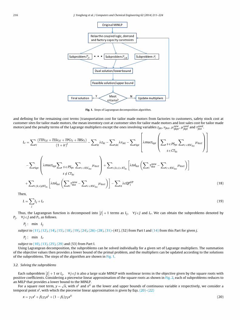
Fig. 1. Steps of Lagrangean decomposition algorithm.

nd defining for the remaining cost terms (transportation cost for tailor made motors from factories to customers, safety stock cost atustomer sites for tailor made motors, the mean inventory cost at customer sites for tailor made motors and lost sales cost for tailor madeotors)and the penalty terms of the Lagrange multipliers except the ones involving variables zjkt , vjkst , �new

ijkpt, �used

jkptand �used

jkst.

Lr =∑

t

(TTFctT + TSSctT + TPCct + TBSct)

(1 + ir)t−∑

kt�zkt −

∑skt

�vskt −∑

kpt

⎡⎢⎢⎣�muctkpt

⎛⎜⎜⎝∑ s ∈ PSps

s ∈ CTks

∑c ∈ KSCksc

�ksct

⎞⎟⎟⎠⎤⎥⎥⎦

−∑

kpt

⎛⎜⎜⎝�muctkpt

∑s ∈ PSps

s /∈ CTks

∑c ∈ KSCksc

�ksct

⎞⎟⎟⎠+

∑t,(k,s) ∈ KTks

[�tolkst

(∑i�new

ikst −∑

c ∈ KSCksc

�ksct

)]

+∑

t,(k,s)/∈KTks

[�tolkst

(∑i�new

ikst −∑

c ∈ KSCksc

�ksct

)]−∑

it�cQPUP

i (18)

Then,

L =∑

j

Lj + Lr (19)

Thus, the Lagrangean function is decomposed into∣∣J∣∣+ 1 terms as Lj, ∀ j ∈ J and Lr. We can obtain the subproblems denoted by

j, ∀ j ∈ J and Pr, as follows.

Pj : min Lj

subject to (11), (12), (14), (15), (18), (19), (24), (26)–(28), (31)–(41), (52) from Part I and (14) from this Part for given j.

Pj : min Lr

subject to (10), (13), (25), (29) and (53) from Part I.Using Lagrangean decomposition, the subproblems can be solved individually for a given set of Lagrange multipliers. The summation

f the objective values then provides a lower bound of the primal problem, and the multipliers can be updated according to the solutionsf the subproblems. The steps of the algorithm are shown in Fig. 1.

.2. Solving the subproblems

Each subproblem∣∣J∣∣+ 1 or Lj, ∀ j ∈ J is also a large scale MINLP with nonlinear terms in the objective given by the square roots with

ositive coefficients. Considering a piecewise linear approximation of the square roots as shown in Fig. 2, each of subproblems reduces ton MILP that provides a lower bound to the MINLP.

For a square root term, y = √x, with xL and xU as the lower and upper bounds of continuous variable x respectively, we consider a

emporal point xt, with which the piecewise linear approximation is given by Eqs. (20)–(22)

x = �1xt + ˇI�2xL + (1 − ˇI)�2xU (20)

J. Yongheng et al. / Computers and Chemical Engineering 62 (2014) 211– 224 217

w

c

xaT

L

3

LesSNNwiiitN

E

wo

a

d

Fig. 2. Piecewise linear approximation of the nonlinear term of the subproblems.

�1 + �2 = 1 (21)

y = �1

√xt + ˇI�2

√xL + (1 − ˇI)�2

√xU (22)

here �1 and �2 are positive continuous variables, ˇI is a binary variable that indicates whether x lies between xL and xt.There are bilinear terms ˇI�2 in Eqs. (20) and (22). We introduce positive continuous variables aI and a′

I as auxiliary variables, andonstraints (23)–(25) as follows.

aI + a′I = �2 (23)

aI ≤ ˇI (24)

a′I ≤ 1 − ˇI (25)

Then, aI = ˇI�2. Hence, Eqs. (20) and (22) can be rewritten as Eqs. (26) and (27).

x = �1xt + aIxL + �2xU − aIx

U (26)

y = �1

√xt + aI

√xL + �2

√xU − aI

√xU (27)

Thus, the square root term y = √x can be approximated with the linear Eqs. (21), (23)–(27).

We adopt an adaptive scheme to update the temporal point. In the first iteration, we take xt = (xL + xU/2), and in the following iterations,t is assigned with the solutions of the previous iteration. This is because the solutions of the previous iteration are close to the real solutions,nd the linear approximation with the temporal point the original upper and lower bounds is relatively accurate near the temporal point.hen, we can expect that xt’s will converge to the optimal solution of the primal problem.

Furthermore, considering that the approximate problems are MILP problems with 0–1 binary and continuous variables, we consider anP relaxation that can provide a lower bound to the MILP, which in turn is a lower bound to the original MINLP.

.3. Feasibility scheme

A feasible solution is necessary to update the upper bound of the primal problem and provide a candidate solution. With the currentagrange multipliers, we can obtain the solutions of the subproblems. But in general, the solutions are not feasible for the primal problem,specially constraints (8) and (9) from Part I are violated, and the value of zjkt and vjkst may not be integer. Therefore, to construct a feasibleolution, we specify zj′kt and vj′′kst with Algorithm Specify.Algorithm Specifytart;oOneU(k, t) = 1;oOneV(k, sp, t) = 1;hile(j ∈ J,

f (z(j, k, t) = maxj′ z(j′, k, t)and NoOneU(k, t) = 1) = 1, then specify z(j, k, t) with 1;f z.l(j, k, t), then NoOneU(k, t) = 0f (vd.l(j, k, sp, t) = maxj′ vd.l(j′, k, sp, t)and NoOneU(k, , sp, t) = 1),hen specify v(j, k, sp, t)with 1;oOneV(k, t)$v.l(j, k, sp, t) = 0

);nd;

In the algorithm, the initial values of z and v come from the corresponding solutions of the subproblems. The algorithm means thate specify zj1kt and vj2kst with 1 for j1 = arg maxj(zjkt) and j2 = arg maxj(vjkst) (if j1 or j2 is not unique, we take the first one by increasing

rder), and specify zjkt (j /= j1) and vjkst (j /= j2) with 0.When zjkt and vjkst are specified with algorithm Specify, the feasibility problem reduces to an MINLP with binary variables, including xijpt

nd yjt, yejt

, yujt

, and continuous variables. The nonlinear terms involve square root functions. To design an efficient feasibility scheme, we

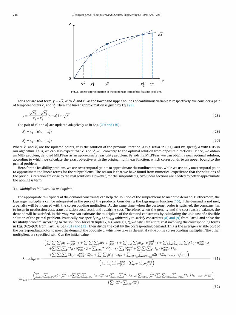
esign another adaptive linear approximation scheme, which is shown in Fig. 3 with xt1 and xt

2 updated iteratively.

218 J. Yongheng et al. / Computers and Chemical Engineering 62 (2014) 211– 224

o

woaap

ttt

3

Latdsfitm

Fig. 3. Linear approximation of the nonlinear term of the feasible problem.

For a square root term, y = √x, with xL and xU as the lower and upper bounds of continuous variable x, respectively, we consider a pair

f temporal points xt1 and xt

2. Then, the linear approximation is given by Eq. (28).

y =√

xt2 −√

xt1

xt2 − xt

1

(x − xt1) +

√xt

1 (28)

The pair of xt1 and xt

2 are updated adaptively as in Eqs. (29) and (30).

x̄t1 = xt

1 + a(xp − xt1) (29)

x̄t2 = xt

2 + a(xp − xt2) (30)

here x̄t1 and x̄t

2 are the updated points, xp is the solution of the previous iteration, a is a scalar in (0,1), and we specify a with 0.05 inur algorithm. Thus, we can also expect that xt

1 and xt2 will converge to the optimal solution from opposite directions. Hence, we obtain

n MILP problem, denoted MILPFeas as an approximate feasibility problem. By solving MILPFeas, we can obtain a near optimal solution,ccording to which we calculate the exact objective with the original nonlinear function, which corresponds to an upper bound to therimal problem.

Here, for the feasibility problem, we use two temporal points to approximate the nonlinear terms, while we use only one temporal pointo approximate the linear terms for the subproblems. The reason is that we have found from numerical experience that the solutions ofhe previous iteration are close to the real solutions. However, for the subproblems, two linear sections are needed to better approximatehe nonlinear term.

.4. Multipliers initialization and update

The appropriate multipliers of the demand constraints can help the solution of the subproblems to meet the demand. Furthermore, theagrange multipliers can be interpreted as the price of the products. Considering the Lagrangean function (15), if the demand is not met,

penalty will be incurred with the corresponding multipliers. At the same time, when the customer order is satisfied, the company haso incur in production cost, transportation cost, stock and repairing cost. Therefore, when the penalty and the cost reach a balance, theemand will be satisfied. In this way, we can estimate the multipliers of the demand constraints by calculating the unit cost of a feasibleolution of the primal problem. Practically, we specify zjkt and vjkst arbitrarily to satisfy constraints (8) and (9) from Part I, and solve theeasibility problem. According to the solution, for each tuple (k, p, t) and (k, s, t), we calculate a total cost involving the corresponding termsn Eqs. (62)–(69) from Part I as Eqs. (31) and (32), then divide the cost by the corresponding demand. This is the average variable cost ofhe corresponding motor to meet the demand, the opposite of which we take as the initial value of the corresponding multiplier. The other

ultipliers are specified with 0 as the initial value.

�muctkp0 = −

(∑i

∑j

∑pgj · �new

ijkpt· � +

∑i

∑j

∑pgpi · �new

ijkpt· � +

∑j ∈ SC

∑pgrjp · �used

jkpt· � +

∑p

∑i

∑j ∈ SC

∑pc1ij · �new

ijkpt· �

+∑i

∑j

∑pc2jk · �new

ijkpt· � +

∑j ∈ SC2 · c2jk · � ·

∑p�used

jkpt+∑

i

∑j

∑p1jp · �new

ijkpt· t1ijp

+∑

i

∑j

∑p2kp · �new

ijkpt· t2jkp +

∑j

∑ph1jp · ssjpt +

∑s/∈KTks

∑cnKSCksc

h2k · �2ks · �ksct ·√

lksct

)(∑

i

∑j

∑p�new

ijkpt+∑

jnSC

∑p�used

jkpt

) (31)

(∑j ∈ SC

∑s ∈ KTks

gr ′js

· �usedjkst

· � +∑

i

∑k

∑s ∈ KTks

c3ik · �newikst

· � +∑

j ∈ SC

∑k2 · c2jk · � ·

∑s ∈ KTks

�usedjkst

+∑

k

∑s ∈ KTks

∑c ∈ KSCksc

h2k · �2ks · �ksct · √mksct

)

�tolkst0 = − (∑

i�new

ikst+∑

j ∈ SC�used

jkst

)(32)

J. Yongheng et al. / Computers and Chemical Engineering 62 (2014) 211– 224 219

1uswns

t

Ti

3

3

oP

m

mt

Fig. 4. Contours of the dual problem.

The subgradient optimization is a common method for updating the set of multipliers for the Lagrangean relaxation (Baker and Sheasby,999). In our problem, a scaling scheme is applied based on the fact that the multipliers of the demand constraints are equivalent to anit cost. Furthermore, there are a large number of multipliers and their values range from the hundreds to the thousands. However, theubgradients of constraint (8) and (9) from Part I cannot exceed the number of warehouses (only 5 warehouses considered in our realorld cases), and the corresponding multipliers are of the same order. This fact tends to make the contours of the dual problem long andarrow, as illustrated in Fig. 4, making the dual problem hard to converge. To overcome the problem, we scale all the multipliers to be theame order of magnitude by scaling so that the contours become near circles. The scaling scheme is as follows.

Recall that L = f (�zkt, �vskt, �muctkpt, �tolkst, �c), and the subgradients of f is g = (gzTkt

, gvTskt

, gmuctTkpt

, gtolTks

, gcT )T.

Let �zkt = ˛z�z′kt

, �vskt = ˛v�v′skt

, �muctkpt = ˛mu�muct′kpt

, �tolks = ˛t�tol′ks

�c = ˛c�c′, where ˛n’s are positive scalars, we can rewrite

he function as L = f ′(�z′kt

, �v′skt

, �muct′kpt

, �tol′ks

, �c′). Then the subgradients of f′ is g′ =(

1˛z

gzTkt

, 1˛v

gvTskt

, 1˛mu

gmuctTkpt

, 1˛t

gtolTks

, 1˛c

gcT)T

.

o make all the multipliers of the same order, we specify ˛v with 1, and ˛z , ˛mu, ˛t , ˛c with 10x which are closest to the correspondingnitial multipliers, where x is an integer, then the multipliers are scaled with Eqs. (33)–(37).

�z′kt = 1

˛z�zkt (33)

�v′skt = 1

˛v�vskt (34)

�muct′kpt = 1

˛mu�muctkpt (35)

�tol′ks = 1˛t

�tolks (36)

�c′ = 1˛c

�c (37)

.5. Lagrangean decomposition algorithm

In summary, the Lagrangean decomposition algorithm is as follows.

.6. Algorithm LD

Step 1: Transform the original MINLP into an MILP, denoted MILPWh, by approximating the square root terms with piecewise linearnes according to Eqs. (21), (23)–(27), and relax all the binary variables to obtain an LP, denoted LPWh; Obtain subproblems Pj, ∀j ∈ J andr of LPWh by relaxing constraints (8) and (9) from Part I;

Step 2: Transform the original MINLP into an MILP, denoted MILPFeas, by approximating the square root terms with a linear approxi-ation according to Eq. (28);

Step 3: Specify zjkt and vjkst arbitrarily subject to constraints (8) and (9) from Part I, then solve MILPWh, and initialize the Lagrange

ultipliers �muctkp and �tolkst according to Eqs. (31) and (32) respectively, initialize the other Lagrange multipliers �z′kt

, �v′skt

, �muct′kpt

, �′

o 0;Step 4: Scale the Lagrange multipliers according to Eqs. (33)–(37);

220 J. Yongheng et al. / Computers and Chemical Engineering 62 (2014) 211– 224

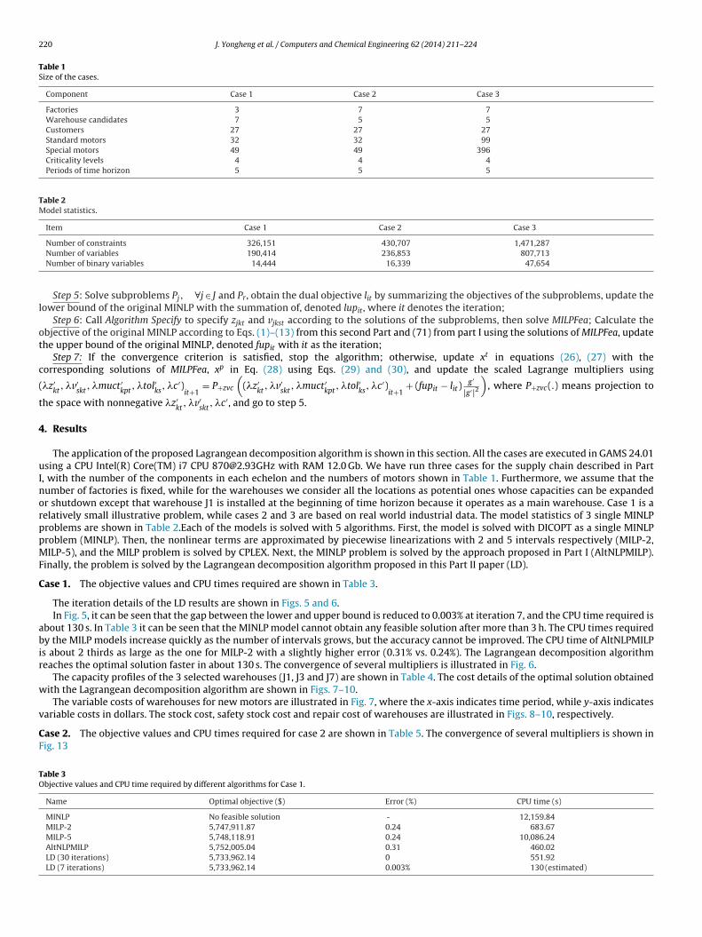
Table 1Size of the cases.

Component Case 1 Case 2 Case 3

Factories 3 7 7Warehouse candidates 7 5 5Customers 27 27 27Standard motors 32 32 99Special motors 49 49 396Criticality levels 4 4 4Periods of time horizon 5 5 5

Table 2Model statistics.

Item Case 1 Case 2 Case 3

l

ot

c

(

t

4

uInorppMF

C

abir

w

v

CF

TO

Number of constraints 326,151 430,707 1,471,287Number of variables 190,414 236,853 807,713Number of binary variables 14,444 16,339 47,654

Step 5: Solve subproblems Pj, ∀j ∈ J and Pr, obtain the dual objective lit by summarizing the objectives of the subproblems, update theower bound of the original MINLP with the summation of, denoted lupit, where it denotes the iteration;

Step 6: Call Algorithm Specify to specify zjkt and vjkst according to the solutions of the subproblems, then solve MILPFea; Calculate thebjective of the original MINLP according to Eqs. (1)–(13) from this second Part and (71) from part I using the solutions of MILPFea, updatehe upper bound of the original MINLP, denoted fupit with it as the iteration;

Step 7: If the convergence criterion is satisfied, stop the algorithm; otherwise, update xt in equations (26), (27) with theorresponding solutions of MILPFea, xp in Eq. (28) using Eqs. (29) and (30), and update the scaled Lagrange multipliers using

�z′kt

, �v′skt

, �muct′kpt

, �tol′ks

, �c′)it+1

= P+zvc

((�z′

kt, �v′

skt, �muct′

kpt, �tol′

ks, �c′)

it+1+ (fupit − lit)

g′

|g′|2)

, where P+zvc(.) means projection to

he space with nonnegative �z′kt

, �v′skt

, �c′, and go to step 5.

. Results

The application of the proposed Lagrangean decomposition algorithm is shown in this section. All the cases are executed in GAMS 24.01sing a CPU Intel(R) Core(TM) i7 CPU 870@2.93GHz with RAM 12.0 Gb. We have run three cases for the supply chain described in Part

, with the number of the components in each echelon and the numbers of motors shown in Table 1. Furthermore, we assume that theumber of factories is fixed, while for the warehouses we consider all the locations as potential ones whose capacities can be expandedr shutdown except that warehouse J1 is installed at the beginning of time horizon because it operates as a main warehouse. Case 1 is aelatively small illustrative problem, while cases 2 and 3 are based on real world industrial data. The model statistics of 3 single MINLProblems are shown in Table 2.Each of the models is solved with 5 algorithms. First, the model is solved with DICOPT as a single MINLProblem (MINLP). Then, the nonlinear terms are approximated by piecewise linearizations with 2 and 5 intervals respectively (MILP-2,ILP-5), and the MILP problem is solved by CPLEX. Next, the MINLP problem is solved by the approach proposed in Part I (AltNLPMILP).

inally, the problem is solved by the Lagrangean decomposition algorithm proposed in this Part II paper (LD).

ase 1. The objective values and CPU times required are shown in Table 3.

The iteration details of the LD results are shown in Figs. 5 and 6.In Fig. 5, it can be seen that the gap between the lower and upper bound is reduced to 0.003% at iteration 7, and the CPU time required is

bout 130 s. In Table 3 it can be seen that the MINLP model cannot obtain any feasible solution after more than 3 h. The CPU times requiredy the MILP models increase quickly as the number of intervals grows, but the accuracy cannot be improved. The CPU time of AltNLPMILP

s about 2 thirds as large as the one for MILP-2 with a slightly higher error (0.31% vs. 0.24%). The Lagrangean decomposition algorithmeaches the optimal solution faster in about 130 s. The convergence of several multipliers is illustrated in Fig. 6.

The capacity profiles of the 3 selected warehouses (J1, J3 and J7) are shown in Table 4. The cost details of the optimal solution obtainedith the Lagrangean decomposition algorithm are shown in Figs. 7–10.

The variable costs of warehouses for new motors are illustrated in Fig. 7, where the x-axis indicates time period, while y-axis indicates

ariable costs in dollars. The stock cost, safety stock cost and repair cost of warehouses are illustrated in Figs. 8–10, respectively.

ase 2. The objective values and CPU times required for case 2 are shown in Table 5. The convergence of several multipliers is shown inig. 13

able 3bjective values and CPU time required by different algorithms for Case 1.

Name Optimal objective ($) Error (%) CPU time (s)

MINLP No feasible solution - 12,159.84MILP-2 5,747,911.87 0.24 683.67MILP-5 5,748,118.91 0.24 10,086.24AltNLPMILP 5,752,005.04 0.31 460.02LD (30 iterations) 5,733,962.14 0 551.92LD (7 iterations) 5,733,962.14 0.003% 130 (estimated)

J. Yongheng et al. / Computers and Chemical Engineering 62 (2014) 211– 224 221

Fig. 5. Convergence of the lower and upper bound for Case 1.

Fig. 6. Convergence of multipliers of demand constraints of motor p1 with criticality k1 at period t for Case 1.

Fig. 7. Variable costs of warehouses for new motor for Case 1.

Fig. 8. Mean stock costs of warehouses for modifying for Case 1.

222 J. Yongheng et al. / Computers and Chemical Engineering 62 (2014) 211– 224

Fig. 9. Safety stock costs of warehouses for Case 1.

Fig. 10. Replace cost of warehouses for special motors for Case 1.

Table 4Capacity profiles of warehouses for Case 1.

SKUs Year 1 Year 2 Year 3 Year 4 Year 5

J1 2000 2000 2000 2000 2000J3 40 40 40 40 40

I

ts

CF

tp

TO

T

J7 50 50 50 50 50

n this case, only J1, J3 and J7 are installed, where the initial capacity of J1 is much larger than the capacities of J3 and J7.

In Fig. 11, it can be seen that the gap between the lower and upper bound is reduced to 0.004% at iteration 8, and the estimated CPUime required is 162 s. There are similar trends as in case 1. The capacity profiles for case 2 of the 3 selected warehouses (J1, J2 and J3) arehown in Table 6 (Fig. 12).

ase 3. The objective values and CPU time required for case 3 are shown in Table 7. The convergence of several multipliers is shown inig. 14

In Fig. 12, it can be seen that the gap between the lower and upper bound is reduced to 0.003% at iteration 7, and the estimated CPUime required is 4696 s. There are similar trends as in case 1. Both MINLP and MILP-5 cannot find any feasible solution, and AltNLPMILPerforms similar to MILP-2 with about twice the CPU time.

able 5bjective values and CPU time required by different algorithms for Case 2.

Name Optimal objective ($) Error (%) CPU time (s)

MINLP 6,537,842.48 5.40 32,288.42MILP-2 6,354,304.15 2.44 798.99MILP-5 6,354,304.15 2.44 86,020.932AltNLPMILP 6,358,672.25 2.51 530.11LD (30 iterations) 6,202,732.33 0 607.58LD (8 iterations) 6,202,732.33 0.004% 162 (estimated)

he iteration details of the LD results are shown in Figs. 11 and 12.

J. Yongheng et al. / Computers and Chemical Engineering 62 (2014) 211– 224 223

Table 6Capacity profiles of warehouses for Case 2.

SKUs Year 1 Year 2 Year 3 Year 4 Year 5

J1 50,000 50,000 50,000 50,000 50,000J2 50 50 50 50 50J3 50 50 50 50 50

Fig. 11. Convergence of lower and upper bound for Case 2.

Fig. 12. Convergence of lower and upper bound for Case 3.

Fig. 13. Convergence of multipliers of demand constraints of motor p1 with criticality k1 at period t for Case 2.

Table 7Objective values and CPU time required by different algorithms for Case 3.

Name Optimal objective ($) Error (%) CPU time (s)

MINLP No feasible solution - 360,123.00MILP-2 120,349,878.7579 11.25 10,871.29MILP-5 No feasible solution - Out of memoryAltNLPMILP 120,657,481.7045 11.53 19,942.81LD (30 iterations) 108,178,792.52 0 20,125.03LD (7 iterations) 108,178,792.52 0.003% 4696 (estimated)

224 J. Yongheng et al. / Computers and Chemical Engineering 62 (2014) 211– 224

rd

Te

5

papcLccvaLctw

A

f

R

BB

FR

M

T

W

Fig. 14. Convergence of multipliers of demand constraints of motor p1 with criticality k1 at period t for Case 3.

From Figs. 5, 11 and 12, we can see that the optimal solutions are all obtained in the early iterations, namely iteration 1, 1, and 3espectively. The reason is that due to the initialization step, the initial Lagrangean multipliers are close to the optimal one, therefore, theualized binary variables obtained by the subproblems and algorithm Specify can reach their optimal values in the early iterations.

To summarize the three cases, we can conclude that the Lagrangean decomposition algorithm can obtain the optimal solution efficiently.he algorithm performs similarly on different scale cases, and as the problem scale increases, the advantage becomes more apparent,specially for highly constrained problems.

. Conclusions

The supply chain of electric motor is complex due to many decisions, especially the reverse flows, which results in a large scale MINLProblem, whose number of variables and equations can range from thousands to millions. Therefore, the solution of this type of problem is

challenging task. Lagrangean decomposition is a popular method for large scale problems, but the decomposition scheme depends on theroblem structure. In this paper, we decompose the problem by warehouses. Given that warehouses share the demands of customers andapacities of factories, the corresponding constraints have to be dualized simultaneously. As a consequence, there are a large number ofagrange multipliers, which are quite different in scale. To accelerate the convergence, a scaling scheme has been proposed. Furthermore,onsidering that the multipliers can be interpreted in an economic sense, we design a method to estimate initial values for them. Anotherhallenge for the decomposition method is that the sizes of the subproblems are still quite large involving nonlinear terms and binaryariables. An adaptive piecewise linearization method is proposed to approximate the nonlinear terms. To obtain feasible solutions, anotherdaptive piece-wise linearization is also presented. The test results on illustrative and real world industrial problems show that theagrangean decomposition algorithm is effective and efficient, while the single MINLP is hard to solve and the MILP approximation is onlyomputationally feasible with a few intervals. The AltNLPMILP of Part I performs similarly to the MILP approximation. The advantage ofhe proposed method is especially apparent for large scale and highly constrained problems. That is, if there are many motors to be dealtith in the supply chain and few potential warehouses to be selected.

cknowledgments

The authors gratefully acknowledge financial support from ABB Corporation, the Center for Advanced Process Decision-MAKING, androm the National Natural Science Foundation of China (No. 61273039).

eferences

aker, B. M., & Sheasby, J. (1999). Accelerating the convergence of subgradient optimization. European Journal of Operational Research, 117, 136–144.uil, R., Piera, M. À., & Luh, P. B. (2012). Improvement of Lagrangian relaxation convergence for production scheduling. IEEE Transactions on Automations Science and Engineering,

9(1), 137–147.umero, F. (2001). A modified subgradient algorithm for Lagrangean relaxation. Computers & Operations Research, 28, 33–52.odriguez, M. A., Vecchietti, A. R., Harjunkoski, I., & Grossmann, I. E. (2013). Optimal supply chain design and management over a multi-period horizon under demand

uncertainty. Part I: MINLP and MILP models. Computers and Chemical Engineering (in press).

ouret, S., Grossmann, I. E., & Pestiaux, P. (2011). A new Lagrangian decomposition approach applied to the integration of refinery planning and crude-oil scheduling.

Computers and Chemical Engineering, 35, 2750–2766.errazas-Moreno, S., Trotter, P. A., & Grossmann, I. E. (2011). Temporal and spatial Lagrangean decompositions in multi-site, multi-period production planning problems with

sequence-dependent changeovers. Computers and Chemical Engineering, 35, 2913–2928.ang, S.-H. (2003). An improved step size of subgradient algorithm for solving the Lagrangian relaxation problem. Computers and Electrical Engineering, 29, 245–249.