optimal stopping and incomplete information in finance - diva portal

U.U.D.M. Report 2011:24

Department of MathematicsUppsala University

Optimal stopping and incomplete information in finance

Bing Lu

Filosofie licentiatavhandling

i matematik

som framläggs för offentlig granskning

den 17 januari, kl 13.15, sal 80127,

Ångströmlaboratoriet, Uppsala

INTRODUCTION

This thesis contains three papers:(1) Recovering a piecewise constant volatility from perpetual put option

prices,(2) Optimal selling of an asset under incomplete information,(3) Optimal selling of an asset with jumps under incomplete information.In the first paper we propose an exact and efficient algorithm for calibra-

tion of a piecewise constant volatility model to a discrete set of perpetualput option prices. In the last two papers we study when to optimally liqui-date an asset under incomplete information in two different settings. In thesecond paper it is assumed that the asset price process follows a geometricBrownian motion with unknown drift, which takes one of two given values.In the third paper we assume that the price process satisfies a jump diffu-sion model with unknown jump intensity taking one of two given values. Weshow that for both cases the optimal liquidation strategy is to sell the assetthe first time the price falls below a time-dependent boundary. We describethe three papers in more detail below.

One of the best known implied volatility models is Dupire’s formula whichwrites the level- and time-dependent volatility in terms of derivatives of Eu-ropean option prices with respect to strike price and maturity. In parallel toDupire’s formula, a level-dependent volatility is expressed by Ekstrom andHobson in terms of perpetual put option prices and their derivatives. How-ever, both models are built on the assumption of a continuum of given optionprices, which is rather unrealistic. In practice, one needs to interpolate be-tween a discrete set of strike prices, and the volatility is very sensitive tothe interpolation procedure. In fact, there are plenty of time-homogeneousmodels that can reproduce the same finite set of perpetual put prices. Anatural candidate is the piecewise constant function of the underlying stockprice, which is studied in the first paper. We start with the forward prob-lem, in which the piecewise constant volatility is given and the prices of theperpetual put option for different strikes are calculated. Then we considerthe inverse problem, in which we construct a piecewise constant volatilitywhich reproduces the given finite set of option prices. The results are alsoillustrated in a numerical example.

The drift of an asset price process is very difficult to estimate from his-torical data. To obtain a decent accuracy in the estimate for the drift, theobservations of the price process for hundreds of years are needed. Thusit is not very realistic to assume that the drift of an asset price process isgiven. In the second paper we study the optimal liquidation problem underthe assumption that the asset price follows a geometric Brownian motion

1

2 INTRODUCTION

with unknown drift, which takes one of two given values. If the drift isknown, then the optimal stopping strategy can be determined immediatelyby simply comparing the drift with the interest rate. In our setting thedrift is not known at the beginning, but an initial estimate of the proba-bilities of both values is given. As time goes by, one can observe the assetprice fluctuations and hence update one’s beliefs about the probabilities forthe drift distribution. First we formulate an optimal stopping problem un-der incomplete information about the drift, and then it is converted into amuch easier problem through the filtering techniques and equivalent measuretransformation for Brownian motion. An early application of the filteringtechniques is the sequential testing of two alternative hypothesis about thedrift of a Brownian motion. The simplified optimal stopping problem, theauxiliary problem, is studied and the optimal liquidation time is the firsttime the point process falls below a certain time-dependent, monotonicallyincreasing and continuous boundary. We also derive an integral equation forthe optimal stopping boundary and study the optimal liquidation problemof closing a short position in the asset.

In option pricing, jump-diffusion processes are widely used to model mar-ket fluctuations. In the third paper we consider the problem of optimalliquidation where the asset price satisfies a jump diffusion model with un-known jump intensity. It is assumed that the intensity takes one of twogiven values and we initially have an estimate of the probabilities of eitherof them. Notice that the problem would be trivial if the jump intensity wasknown. Although complete information of the intensity is not available atthe beginning, one can observe the asset price process, and learn more aboutthe distribution of the intensity. The equivalent measure transformations forjump processes with stochastic intensity as well as for compound Poissonprocesses and the filtering techniques for point processes are used here tosimplify the problem. An early application of the filtering techniques is thesequential testing of two alternative hypothesis about the jump intensityof a Poisson process. The best liquidation strategy is to sell the asset thefirst time the counting process falls below or goes above a time-dependentmonotone boundary, which depends on the distribution of the jump size ofthe compound Poisson process.

RECOVERING A PIECEWISE CONSTANT VOLATILITY FROM

PERPETUAL PUT OPTION PRICES

BING LU

Abstract. In this paper we present a method to recover a time-homogeneouspiecewise constant volatility from a finite set of perpetual put option prices.The whole calculation process of the volatility is decomposed into easy com-putations in many fixed disjoint intervals. In each interval, the volatility isobtained by solving a system of nonlinear equations.

1. Introduction

One of the most studied problems in mathematical finance is to calculate theprice of an option if the diffusion coefficient of the underlying asset is given. Inpractice, it is often natural to consider the inverse problem: how to compute thevolatility of the underlying stock price if a set of option prices is provided. Forexample, in the classical Black-Scholes model there is a unique correspondencebetween the constant volatility and the price of a European option. Thus, theimplied volatility can be obtained by the Black-Scholes formula if one option priceis known. In general, however, if more than one option price is given, a richer modelis needed for the underlying process. One such model is the local volatility model,in which the volatility depends on the current stock price and the current time.Also this model can be calibrated to fit given option data perfectly. Indeed, Dupire[3] showed that the level- and time-dependent volatility can be written in terms ofderivatives of European option prices with respect to strike price and maturity.

In the present paper we are interested in calibration of models from the pricesof perpetual American put options. The volatility of the underlying is consideredto be time-homogeneous. Similar to the European case mentioned above, if theBlack-Scholes model is offered as the process of the underlying stock price, then itis straightforward to compute the constant volatility if one option price is given.In parallel to the Dupire’s equation, a level-dependent model for the stock priceis created by Ekstrı¿1

2m and Hobson(2009), see also Alfonsi and Jourdain [1]. Ek-

strı¿12m and Hobson assume that the prices of the perpetual put options are given

for all different strike prices and they express the diffusion coefficient in terms ofthe option prices and their derivatives. This volatility is uniquely determined atthe price level below the current stock price.

As noted above, both Dupire’s formula for the volatility and the level-dependentvolatility recovered from prices of perpetual put options are calculated under anassumption of a (possibly double) continuum of given option prices. In reality,however, option prices are only given for a discrete set of strike prices, so one thenneeds to interpolate between them. Moreover, since the volatility is calculated using

Key words and phrases. Perpetual put options; Calibration of models; Piecewise constantvolatility.

1

2 BING LU

derivatives of the option prices, it is very sensitive to the interpolation procedure.On the other hand, the constant volatility defined in the Black-Scholes model iseasy to calculate, but generically it is impossible to fit one constant volatility ifseveral option prices are given.

Motivated by the discussion above, we consider a situation in which prices ofperpetual American put options are given for a finite set of strike prices. To ruleout arbitrage possibilities, the option price has to be increasing and convex in thestrike. Moreover, we assume that the option price is strictly convex in strikes.Since there does not exist a continuum of option prices, one can create plenty oftime-homogeneous models to reproduce the option data (one for each choice ofinterpolation procedure). A natural candidate for the time-homogeneous volatilitymodel is the piecewise constant function of the stock price. In the present paperwe prove the existence of a piecewise constant volatility that reproduces the givenoption prices. Given n option prices, the whole calculation process is decomposedinto elementary computation in n fixed disjoint intervals. To obtain the volatilityin each interval, one just needs to solve two nonlinear equations with two unknownvariables. Moreover, since it does not involve differentiation of the option price, webelieve that it is more stable with respect to small changes in the input than themodel by Ekstrı¿1

2m and Hobson.The paper is organized as follows. In Section 2, we study the forward problem.

Provided that the volatility is a piecewise constant function of the underlying stockprice, we can calculate the price of the perpetual put option for different strikeprices. Section 3 treats the inverse problem and contains our main results. Given afinite set of prices of the perpetual put options, we present a method to construct apiecewise constant volatility which reproduces the option prices. In Section 4, theresults are illustrated in a numerical example.

2. The Forward Problem

We consider a model where the process of the stock price X solves the stochasticdifferential equation

dXt = rXtdt+ σ(Xt)XtdWt.

Here r is the constant interest rate, W is the standard Brownian motion and σ(Xt)is a positive function. Given the current stock price x0, the price of a perpetualAmerican put option with strike K is

P (K) = supτ

Ex0 [e−rτ (K −Xτ )+],(1)

where τ is any stopping time with respect to the filtration generated by W . Thesolution to the optimal stopping problem (1) is closely related to the ordinarydifferential equation

1

2σ2(x)x2uxx + rxux − ru = 0.(2)

There are two linearly independent solutions to this ODE. If one of them is positiveand increasing and the other one positive and decreasing, then they are unique upto positive multiplicative constants, compare [2] pages 18-19. We denote these solu-tions by ψ and ϕ, respectively. Without loss of generality, we choose the decreasingsolution to satisfy ϕ(x0) = 1. Define the hitting times Hz = inft ≥ 0 : Xt = z.

RECOVERING A PIECEWISE CONSTANT VOLATILITY FROM PERPETUAL PUT OPTIONS3

Since e−rtϕ(Xt) is a local martingale and ϕ(x) is decreasing in x, we have

Ex[e−rHz ] =ϕ(x)

ϕ(z)if x > z .

Due to the time-homogeneity of problem (1), it suffices to take the supremum overstopping times that are exit times from an interval. Moreover, since put optionsare considered, we only need to take the supremum over hitting times Hz for somelevel z, compare the proof of Lemma 2.2 in [4]. We thus find

P (K) = supτ

Ex0 [e−rτ (K −Xτ )+]

= supz:z≤x0∧K

Ex0 [e−rHz(K −XHz)+]

= supz:z≤x0∧K

(K − z)Ex0[e−rHz ]

= supz:z≤x0

K − z

ϕ(z).

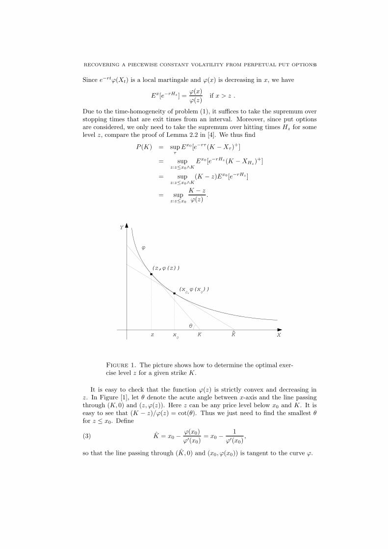
Figure 1. The picture shows how to determine the optimal exer-cise level z for a given strike K.

It is easy to check that the function ϕ(z) is strictly convex and decreasing inz. In Figure [1], let θ denote the acute angle between x-axis and the line passingthrough (K, 0) and (z, ϕ(z)). Here z can be any price level below x0 and K. It iseasy to see that (K − z)/ϕ(z) = cot(θ). Thus we just need to find the smallest θfor z ≤ x0. Define

(3) K = x0 −ϕ(x0)

ϕ′(x0)= x0 −

1

ϕ′(x0),

so that the line passing through (K, 0) and (x0, ϕ(x0)) is tangent to the curve ϕ.

4 BING LU

When K ≤ K, it is not optimal to exercise the option immediately. Instead,the investors should wait until the stock price hits the optimal stopping level toexercise the option. Thus we have

P (K) = supz

K − z

ϕ(z),(4)

where the optimal z, which is the optimal exercise level for strike K, is chosen sothat

(K − z)ϕ′(z) + ϕ(z) = 0.(5)

Equation (5) indicates that the straight line passing through (K, 0) and (z, ϕ(z))

is tangent to the function ϕ. We also obtain P (K) = K − x0 for K > K, whichimplies that it is optimal for investors to exercise the option immediately.

We now specialize to the case of piecewise constant volatility. More precisely,it is assumed that the interval [0, x0] is divided by a mesh consisting of n pointsa1, a2, a3...an, which satisfy 0 < a1 < a2...an−1 < an ≤ x0. The volatility functionσ(Xt) is defined as

σ(x) =

σ0, 0 < x < a1σi, ai ≤ x < ai+1, 1 ≤ i ≤ n− 1σn, an ≤ x

(6)

where σ0, ..., σn are positive constants. On an interval (ai, ai+1), the volatility isconstant and therefore the fundamental solution ϕ is C∞. However, at a jump pointai of σ, the function ϕ is merely C1 and the second derivative has a jump. Giventhe piecewise constant volatility function σ(x) defined above, the two independentpositive solutions of the ODE (2) are

ψ(x) = x

and

ϕ(x) =

A0x−β0 +B0x, 0 < x < a1

Aix−βi +Bix, ai ≤ x < ai+1, 1 ≤ i ≤ n− 1

Anx−βn +Bnx, an ≤ x

(7)

where βi = 2r/σ2i for i ∈ 0, ..., n. Here Ai and Bi for i ∈ 0, ..., n are chosen so

that ϕ(x) is C1 everywhere. Without loss of generality, we let ϕ(x0) = 1, thus

An = xβn

0 , Bn = 0,(8)

since ϕ(x) is decreasing and non-negative for x ≥ an. Due to the C1-regularity, wehave

Aia−βi

i+1 +Biai+1 = Ai+1a−βi+1

i+1 +Bi+1ai+1

−Aiβia−βi−1i+1 +Bi = −Ai+1βi+1a

−βi+1−1i+1 +Bi+1.

It follows that

Ai = Ai+1aβi−βi+1

i+11+βi+1

1+βi

Bi = Ai+1a−βi+1−1i+1

βi−βi+1

1+βi+Bi+1.

(9)

for i ∈ 0, ..., n− 1.


The function ϕ(x) defined in (7), (8) and (9) is the decreasing fundamental

solution to the ODE (2). Hence, for K ≤ K = x0(1 + 1/βn) the option price is

P (K) = supz

K − z

ϕ(z),(10)

where the optimal z is determined by

(K − z)ϕ′(z) + ϕ(z) = 0.(11)

For K > K we have P (K) = K − x0. Since ϕ(x) is C1 and strictly convex in x,

equation (11) defines a one-to-one correspondence between strike prices K ∈ (0, K]and optimal exercise levels z ∈ (0, x0]. Now let K∗

i be the strike price for which aiis the optimal exercise level. By (11), we have

K∗

i = − ϕ(ai)

ϕ′(ai)+ ai =

(1 + βi)Ai

βiAia−1i −Bia

βi

i

.(12)

for 1 ≤ i ≤ n. It is straightforward to find that

K∗

n = an(1 + βn)/βn(13)

Since K is strictly increasing as a function of z, we have that K∗

i is increasing ini. Moreover, for K ∈ [K∗

i ,K∗

i+1), the optimal exercise level z belongs to [ai, ai+1).By summarizing all our findings in this section, we obtain the following theorem.

Theorem 1. Given the piecewise constant volatility defined in (6), the price of the

perpetual American put option defined by (1) is given by

P (K) =

K − x0, K ≥ KKβn+1ββn

n

xβn0

(1+βn)1+βn, K∗

n ≤ K < KK−z

Aiz−βi+Biz

, K∗

i ≤ K < K∗

i+1, 1 ≤ i ≤ n− 1K−z

A0z−β0+B0z

, 0 < K < K∗

1 .

(14)

Here Ai and Bi for i ∈ 0, ..., n− 1 are defined by (9). The optimal exercise level

z in (14) is determined implicitly by

(K − z)(−Aiβiz−βi−1 +Bi) +Aiz

−βi +Biz = 0(15)

if K ∈ [K∗

i ,K∗

i+1) for i ∈ 1, ..., n− 1 or if K < K∗

1 for i = 0.

By the theorem, the option price P (K) can be computed explicitly if a piecewiseconstant volatility σ(x) is given as in equation (6).

3. The Inverse Problem

In this section, we take the point of view that option prices for a discrete setof strikes written on a certain underlying asset can be recorded from the market.We construct a piecewise constant volatility function of the underlying stock price,which is calibrated to perfectly fit the finite set of option prices.

Assume that n strike prices and the corresponding n perpetual put option pricesare given from the market data. Arbitrage considerations give that the put optionprice has to be non-decreasing and convex inK. Below we make the slightly strongerassumptions that it is increasing and strictly convex. Thus the option price P (Ki)has to satisfy

P (K1) < P (K2) < ... < P (Kn)(16)

6 BING LU

for the strike prices 0 < K1 < K2 < ... < Kn. For the index level n, we assumethat Kn satisfies P (Kn) = Kn − x0, where x0 is the current stock price. Below Kn

will correspond to K in the forward problem, so any option with strike price that isbigger than or equal to Kn should be exercised immediately. Later in this sectionwe will discuss the case when Kn can not be observed from the market. We alsoassume that the natural bounds

(Ki − x0)+ < P (Ki) < Ki(17)

for i ∈ 1, ..., n − 1 are fulfilled, where the first strict inequality implies that itis not optimal to exercise the option immediately. We also assume that the valuefunction P (K) is strictly convex in the strikes, so that

P (K2)− P (K1)

K2 −K1>P (K1)

K1(18)

and

P (Ki)− P (Ki−1)

Ki −Ki−1<P (Ki+1)− P (Ki)

Ki+1 −Ki

(19)

for i ∈ 2, ..., n− 1. It follows thatP (Ki)− P (Ki−1)

Ki −Ki−1< 1.(20)

for i ∈ 2, ..., n.Next we will draw a graph containing all the information given by (16), (17), (18),(19) and (20). In the x-ϕ(x) coordinate system, draw the lines passing through(Ki, 0) with slope −1/P (Ki) for every i ∈ 1, ..., n. We refer to those lines as”option lines” and denote the option line with index level i by li. According toequation (19), we have

Ki −Ki−1

P (Ki)− P (Ki−1)>

Ki+1 −Ki

P (Ki+1)− P (Ki),

where the expression on the left hand side is the second coordinate of the intersec-tion between li and li−1, and the expression on the right hand side is the secondcoordinate of the intersection between li+1 and li.According to equation (18), we obtain

K2 −K1

P (K2)− P (K1)<

K1

P (K1),

which implies that the second coordinate of the intersection between l2 and l1is smaller than the second coordinate of the intersection between l1 and ϕ(x)-axis. Therefore, as i decreases from n to 2, the first and the second coordinate ofthe intersection between li and li−1 are all positive and decreases and increases,respectively. Equation (17) gives

Ki − x0P (Ki)

< 1

for any i ∈ 1, ..., n − 1, which implies that (x0, 1) is on the right side of all theoption lines except ln. Note that the point (x0, 1) is on ln. According to (20), wehave

Kn −Kn−1

P (Kn)− P (Kn−1)> 1.


This shows that the second coordinate of the intersection between ln and ln−1 islarger than 1. Summing up all the information mentioned above, Figure [2] gives asimple version of option lines.

Figure 2. The option line li has slope −1/P (Ki) and intersectsthe x-axis in the point (Ki, 0).

Theorem 2. Assume that n strike prices K1, ...,Kn and the corresponding prices

of perpetual put options P (K1), ..., P (Kn) satisfying the conditions (16), (17), (18),(19), (20) and P (Kn) = Kn − x0 are given, where x0 is the current stock price.

Then there exists a time-homogeneous process with a piecewise constant volatility

that recovers the option prices.

Proof. We are looking for a piecewise constant volatility of the form

σ(x) =

σ0, 0 < x < b1σi1, bi ≤ x < ci, 1 ≤ i ≤ n− 1σi2, ci ≤ x < bi+1, 1 ≤ i ≤ n− 1σ∗, x ≥ bn = x0,

(21)

where 0 < b1 < c1 < ... < bi < ci < bi+1 < ... < bn = x0. With this volatility, thedecreasing fundamental solution to the ODE (2) is of the form

ϕ(x) =

A0x−β0 +B0x, 0 < x < b1

Ai1x−βi1 +Bi1x, bi ≤ x < ci, 1 ≤ i ≤ n− 1

Ai2x−βi2 +Bi2x, ci ≤ x < bi+1, 1 ≤ i ≤ n− 1

A∗x−β∗

+B∗x, x0 ≤ x

(22)

where β0 = 2r/σ20 (and similarly for βi1, βi2 and β∗). The constants A0, Ai1, Ai2,

A∗, B0, Bi1, Bi2 and B∗ should be chosen so that ϕ(x) is C1 everywhere. If one

8 BING LU

can find a function ϕ(x) of the form (22) with suitable parameters which is tangentto all the option lines and touching the point (x0, 1) and the first coordinates ofthose tangent points are not bigger than x0, then it satisfies

P (Ki) = supz

Ki − z

ϕ(z),

and the optimal z for each Ki is smaller than or equal to x0. Hence, the cor-responding piecewise constant volatility σ(x) is calibrated to fit the set of optionprices perfectly and is the volatility that we are looking for.Next we are going to determine bi for i ∈ 1, ..., n and ci for i ∈ 1, ..., n− 1.Let di be the first coordinate of the intersection of li and li+1. Thus we have

di =KiP (Ki+1)−Ki+1P (Ki)

P (Ki+1)− P (Ki)(23)

for i ∈ 1, ..., n− 1. Choose bi to be

bi =di−1 + di

2(24)

for i ∈ 2, ..., n − 1, and b1 = d1/2 and bn = x0. We will construct ϕ so that biis the first coordinate of the tangent point where ϕ touches the li. (In fact thistangent point could be chosen anywhere on the segment that connects the nearesttwo intersections, but we believe that the mid-point is a natural choice. For b1, onemay argue that b1 = 2d1 − b2 is another natural choice in some cases.) The secondcoordinate of the tangent point corresponding to bi is

ϕ(bi) =(Ki −Ki−1)(P (Ki+1)− P (Ki))

2(P (Ki)− P (Ki−1))(P (Ki+1)− P (Ki))(25)

+(Ki+1 −Ki)(P (Ki)− P (Ki−1))

2(P (Ki)− P (Ki−1))(P (Ki+1)− P (Ki))

for i ∈ 2, ..., n− 1, which can be easily computed by plugging in the option data.Additionally, we have

ϕ(b1) =2K1 − d12P (K1)

, ϕ(bn) = 1.(26)

For simplicity, we let ci equal di defined in equation (23). For a graphic illustrationof the choices of bi and ci, see Figure [3].

In the interval [bi, bi+1) for i ∈ 1, .., n − 1 the function ϕ(x) should be C1,which implies the following equations

ϕ(bi) = Ai1bi−βi1 +Bi1bi

∂ϕ(x)

∂x|x=bi = −βi1Ai1bi

−βi1−1 +Bi1 = − 1

P (Ki)

ϕ(bi+1) = Ai2bi+1−βi2 +Bi2bi+1

∂ϕ(x)

∂x|x=bi+1

= −βi2Ai2bi+1−βi2−1 +Bi2 = − 1

P (Ki+1)

ϕ(ci) = Ai1ci−βi1 +Bi1ci = Ai2ci

−βi2 +Bi2ci

∂ϕ(x)

∂x|x=ci = −βi1Ai1ci

−βi1−1 +Bi1 = −βi2Ai2ci−βi2−1 +Bi2.


Figure 3. The break point ci is chosen as the first coordinate ofthe intersection between li and li+1. The break point bi is chosenas the average of ci−1 and ci.

Let ϕ(x, βi1) = ϕ(x) be a function of the variables x and βi1 for x ∈ [bi, ci] andϕ(x, βi2) = ϕ(x) be a function of the variables x and βi2 for x ∈ [ci, bi+1). Notethat ϕ(bi) and ϕ(bi+1) are constants that we can compute, ϕ(x) is a function ofthe variable x and ϕ(x, βi1) (ϕ(x, βi2)) is a function with variables x and βi1 (βi2).After some manipulation the six equations become

ϕ(x, βi1) = ϕ(bi)P (Ki)+bi(1+βi1)P (Ki)

( bix)βi1 + P (Ki)βi1ϕ(bi)−bi

P (Ki)(1+βi1)xbi,

bi ≤ x < ciϕ(x, βi2) = ϕ(bi+1)P (Ki+1)+bi+1

(1+βi2)P (Ki+1)( bi+1

x)βi2

+P (Ki+1)βi2ϕ(bi+1)−bi+1

P (Ki+1)(1+βi2)x

bi+1

, ci ≤ x ≤ bi+1

ϕ(ci, βi1) = ϕ(c1, βi2)∂ϕ(x,βi1)

∂x|x=ci = ∂ϕ(x,βi2)

∂x|x=ci,

(27)

for i ∈ 1, .., n − 1. The option prices P (Ki) and Ki for i ∈ 1, ..., n are givenand it is straightforward to compute ci, bi and ϕ(bi) for each i, so in each interval[bi, bi+1) there are only two unknown parameters βi1 and βi2 to be determined.Next we will prove the existence of a solution to the system of equations (27).It is easy to check that

limβi1→0

ϕ(x, βi1) = ϕ(bi)−x− biP (Ki)

,

10 BING LU

which implies that ϕ(x, βi1) tends to li as βi1 goes to zero. Similarly, one can showthat ϕ(x, βi2) tends to li+1 as βi2 goes to zero. We can also check that

limβi1→∞

ϕ(x, βi1) =ϕ(bi)x

bi, lim

βi2→∞

ϕ(x, βi2) → ∞.

Claim 1. The functions ϕ(x, βi1) and ϕ(x, βi2) are increasing in βi1 and βi2, re-spectively.

Proof of the claim. For x ∈ [bi, ci), define z = bi/x. Then

ϕ(x, βi1) =ϕ(bi)P (Ki) + bi(1 + βi1)P (Ki)

zβi1 +P (Ki)βi1ϕ(bi)− bizP (Ki)(1 + βi1)

.

Taking derivative of ϕ(x, βi1) with respect to βi1 yields

1 + βi1

ϕ(bi) +bi

P (Ki)

∂ϕ(x, βi1)

∂βi1= zβi1 ln z +

1

1 + βi1(1

z− zβi1) = f(z).

Note that 0 < z ≤ 1 and f(1) = 0. Thus in order to show that ϕ(x, βi1) is increasingin βi1, it suffices to show that f(z) is positive for 0 < z < 1. Next differentiatingzf(z) with respect to z gives

∂(zf(z))

∂z= (1 + βi1)z

βi1 ln z < 0

for 0 < z < 1. Note that 1× f(1) = 0, thus zf(z) > 0 for 0 < z < 1. It follows thatf(z) > 0 for 0 < z < 1, which implies that ∂ϕ(x, βi1)/∂βi1 > 0. One can also showthat ∂ϕ(x, βi2)/∂βi2 > 0 by a similar argument as above. This finishes the proofof the claim.

Therefore as βi1 increases from zero to infinity, ϕ(x, βi1) increases from ϕ(bi)−x−biP (Ki)

to ϕ(bi)xbi

. Again as βi2 increases from zero to infinity, ϕ(x, βi2) also increases

from ϕ(bi+1) − x−bi+1

P (Ki+1)to infinity. Let A be the point (ci,

Ki−ciP (Ki)

) and B be the

point (ci,ϕ(bi)(bi+1−ci)+ϕ(bi+1)(ci−bi)

bi+1−bi), compare Figure [4]. If we choose a point on

the segment AB except for the point A, then there exist βi1 and βi2 such thatϕ(x, βi1) and ϕ(x, βi2) pass through that point. For βi1 and βi2 sufficiently small,ϕ(x, βi1) and ϕ(x, βi2) will meet at some point at the segment AB which is veryclose to the point A. Clearly, the angle between ϕ(x, βi1) and ϕ(x, βi2) is smallerthan 180, compare Figure [4]. If ϕ(x, βi1) and ϕ(x, βi2) meet at point B, the anglebetween the two ϕ functions is larger than 180 due to the convexity of ϕ(x, ·) inx. As the intersection of the two ϕ functions moves from A to B along the segmentAB, the angle between the two ϕ functions increases from less than 180 to morethan 180. Hence, by a continuity argument, there exists a point on the segmentAB such that the angle between the two ϕ functions is exactly 180. For thisparticular choice of βi1 and βi2, define ϕ by ϕ(x) = ϕ(x, βi1) for x ∈ [bi, ci] andϕ(x) = ϕ(x, βi2) for x ∈ [ci, bi+1). In this way, ϕ is C1 at ci. This finishes the proofof the existence of βi1 and βi2 for i ∈ 1, ..., n− 1.

Note that β0 only influences the prices of options with K < K1 which are notgiven. Thus β0 can be defined arbitrarily. For simplicity, we let β0 = β11. It followsthat A0 = A11 and B0 = B11. Since ϕ(x) is C

1 and decreasing in x and ϕ(x0) = 1,

it is easy to calculate that β∗ = x0/P (Kn), B∗ = 0 and A∗ = x0

β∗

.


Figure 4. The existence of βi1 and βi2

According to (27), in the interval [bi, bi+1) for i ∈ 1, ..., n− 1, we just need tosolve the two nonlinear equations

ϕ(bi)P (Ki) + bi(1 + βi1)P (Ki)

(bici)βi1 +

P (Ki)βi1ϕ(bi)− biP (Ki)(1 + βi1)

cibi

(28)

=ϕ(bi+1)P (Ki+1) + bi+1

(1 + βi2)P (Ki+1)(bi+1

ci)βi2 +

P (Ki+1)βi2ϕ(bi+1)− bi+1

P (Ki+1)(1 + βi2)

cibi+1

and

−βi1ϕ(bi)P (Ki) + bi(1 + βi1)P (Ki)

(bici)βi1

1

ci+P (Ki)βi1ϕ(bi)− bibiP (Ki)(1 + βi1)

(29)

= −βi2ϕ(bi+1)P (Ki+1) + bi+1

(1 + βi2)P (Ki+1)(bi+1

ci)βi2

1

ci+P (Ki+1)βi2ϕ(bi+1)− bi+1

bi+1P (Ki+1)(1 + βi2).

to obtain the volatility.

Theorem 3. Assume that n strike prices K1, ...,Kn and the corresponding prices

of perpetual put options P (K1), ..., P (Kn) satisfying the conditions specified in The-

orem 2 are given. The piecewise constant volatility that recovers the option prices

can be computed by the following procedure:

(1) Calculate ci, bi and ϕ(bi) for each i by equations (23), (24), (25) and (26).Additionally, let b1 = c1/2 and bn = x0.(2) Plug the numbers computed above into (28) and (29) to obtain βi1 and βi2 for

i ∈ 1, ..., n− 1. The tail volatility β∗ = x0/P (Kn) and let β0 = β11.Then the piecewise constant volatility that recovers the given option prices is given

12 BING LU

by

σ(x) =

√

2rβ0

, 0 ≤ x < b1√

2rβi1, bi ≤ x < ci for 1 ≤ i ≤ n− 1

√

2rβi2, ci ≤ x < bi+1 for 1 ≤ i ≤ n− 1

√

2rβ∗, x0 ≤ x.

Remark 1. Note that the volatility model described above is not the unique piece-

wise constant volatility model that reproduces the option data. In fact, the choice of

the break points bi and ci is arbitrary to some extent. For example, our assumption

that the tangent point where ϕ touches the option line is located in the middle of

two intersections could easily be changed, thereby giving rise to a different volatility.

Also note that we obtain 2n constant volatilities from n option prices, so the degree

of freedom is n. However, it seems difficult for us to both decrease the degree of

freedom and at the same time ensure the solvability of the problem.

It might happen that Kn satisfying P (Kn) = Kn − x0 can not be observed fromthe market. In such a case, to apply the calibration method described above, wemust make up a proper Kn with P (Kn) = Kn − x0 using the given option dataP (K1), ..., P (Kn−1). Since P (K) is strictly convex with respect to K, the strikeprice Kn has to satisfy

Kn − x0 > P (Kn−1) + (Kn −Kn−1)P (Kn−1)− P (Kn−2)

Kn−1 −Kn−2.(30)

There are many ways of choosing Kn that satisfies (30). For example, one waywould be to use a second order Taylor expansion of P at the point Kn−1. However,we omit the details of this procedure.

4. Numerical illustration

In the numerical test, we assume that option data observed in the market are

actually calculated using a CEV-model with σ(x) = x−1

2 . Let the current stockprice be x0 = 10, the interest rate be r = 0.1, then the ϕ function (compare [2]pages 18-19) is given by

ϕ(x) = 26.6423x

∫

∞

x

1

y2e−0.2y dy.(31)

According to (3) and (31), we obtain that K = 13.8778. A series of strike pricesKi between 3 and 13.8778 are selected as option data, and the correspondingseries of option prices P (Ki) can be computed by equation (10) and (11). Thevolatility (the solid curve) produced by Theorem 3 is plotted comparing to the realvolatility (the dotted curve) in Figure [5]. As the number of option prices givenincreases, our predicted volatility fits better and better with the given volatility.

References

[1] Alfonsi, A and Jourdain, B (2009) Exact volatility calibration based on a Dupire-type

Call-Put duality for perpetual American options, Nonlinear Differential Equations and Ap-plications 16, 523-554.

[2] Borodin, A. and Salminen, P. (2002). Handbook of Brownian motion-facts and formula,

Birkhı¿ 1

2user Verlag, Basel.

[3] Dupire, B. (1994) Pricing with a smile. Risk 7, 18-20


0 5 10 150

0.5

1

1.5

2

2.5

3

3.5

(a) 10 pairs of option data

0 5 10 150

0.5

1

1.5

2

2.5

3

3.5

(b) 100 pairs of option data

Figure 5. The dotted line is the real volatility σ(x) = x−1/2, andthe solid line is the computed volatility.

[4] Ekstrı¿ 1

2m, E. and Hobson, D. (2009) Recovering A Time-Homogeneous Stock Price Pro-

cess From Perpetual Option Prices. Preprint.

Department of Mathematics, Box 480, 75106 Uppsala, Sweden

E-mail address: [email protected]

OPTIMAL SELLING OF AN ASSET UNDER INCOMPLETE

INFORMATION

ERIK EKSTROM1 AND BING LU

Abstract. We consider an agent who wants to liquidate an asset withunknown drift. The agent believes that the drift takes one of two givenvalues, and has initially an estimate for the probability of either of them.As time goes by, the agent observes the asset price and can thereforeupdate his beliefs about the probabilities for the drift distribution. Weformulate an optimal stopping problem that describes the liquidationproblem, and we demonstrate that the optimal strategy is to liquidatethe first time the asset price falls below a certain time-dependent bound-ary. Moreover, this boundary is shown to be monotonically increasing,continuous and to satisfy a non-linear integral equation.

1. Introduction

This paper treats the problem of optimal timing for an irreversible sale ofan indivisible asset under incomplete information about its drift. The assetprice is assumed to follow a geometric Brownian motion X with unknowndrift, and an agent who decides to sell at time t receives at this time theamount Xt. The objective of the agent is to choose a liquidation time forwhich the expected value of the (discounted) asset price is maximised. Suchproblems are important for all types of investors with insufficient knowledgeof the future trend of an asset.

In the case with complete information about the model parameters ofX, the corresponding optimal liquidation problem is trivial. Indeed, if thedrift is larger than the interest rate, then on average the asset price growsfaster than money in a risk-free bank account, and the agent should keepthe asset as long as possible. Similarly, a drift smaller than the interest rateimplies that the agent should liquidate the asset immediately and insteaddeposit the money in the bank. However, we remark that the assumptionof complete information about the parameters of X is quite strong. Thevolatility of an asset can, at least in principle, be estimated instantaneouslyby observing the price fluctuations over an arbitrarily short time period. Onthe other hand, the drift is notoriously difficult to estimate from historical

Date: August 5, 2011.Key words and phrases. Optimal liquidation of an asset; incomplete information; opti-

mal stopping.1 Support from the Swedish Research Council (VR) is gratefully acknowledged.

1

2 ERIK EKSTROM AND BING LU

data, and to achieve a decent accuracy in the estimate for the drift onetypically needs observations of the process from hundreds of years.

Instead, we allow for incomplete information by modelling the drift as arandom variable which is not directly observable for the agent. Initially, theagent’s beliefs about the drift are summarised by a probability distribution.As time goes by, however, he observes the asset price process, and based onthese observations his beliefs may change. Naturally, if the asset price risesquickly, then the agent will consider it more likely that the drift takes thelarger of the two values, and he would postpone the liquidation. Similarly, ifthe asset falls drastically, then it is likely that the true drift is small, and theagent would be more inclined to liquidate his position early. We show belowthat this intuition is true, i.e. there exists a boundary between the continu-ation region and the stopping region such that the optimal liquidation timecoincides with the first time the asset price falls below the boundary. Wealso derive monotonicity and continuity properties of the boundary, and weshow that it satisfies a non-linear integral equation similar to the one whichcharacterises the optimal stopping boundary for the American put option.

Related problems of liquidating an indivisible asset have been studied in[4] and [7]. These papers study a risk-averse agent who wants to sell anindivisible asset with the possibility of hedging some of the risk by investingin a correlated stock market. The paper [2], see also [6], studies a problemof optimal selling of an asset, where optimality is measured by closenessbetween the current asset price and its ultimate maximum over the wholetime period. In all the papers refered to above, the agent is assumed to havecomplete information about the underlying price processes. The methodswe use to treat the incomplete information in our setting are standard andbased on filtering theory, see for example [12]. An early application of thesetechniques is the sequential testing of two alternative hypothesis about thedrift of a Brownian motion; for further details and related references seeChapter VI.21 in [14]. Similar techniques to tackle investment problems inmarkets with incomplete information are also applied in [9] and [11], wherethe problem of maximising expected utility of terminal wealth by trading indifferent assets is studied. The papers [1] and [10] study the optimal tim-ing for an investment under incomplete information. Mathematically, theinvestment problem in [1] is equivalent to the pricing of an American calloption written on an asset with unknown drift. Using filtering techniques,the problem is reduced to an optimal stopping problem with complete infor-mation, but with two underlying spatial dimensions. A clever observationin [10] reduces the two-dimensional problem into a one-dimensional optimalstopping problem, but in general for a time-dependent pay-off function (forone specific choice of parameters, however, the time dependence disappearsand the optimal stopping problem can be solved explicitly). In the presentpaper, the optimal liquidation problem has a linear pay-off, which impliesthat the problem can be reduced to a one-dimensional optimal stopping

OPTIMAL SELLING OF AN ASSET UNDER INCOMPLETE INFORMATION 3

problem for a time-homogeneous diffusion with an affine pay-off regard-less of what parameters are chosen. Consequently, this reduced problem isstraightforward to analyse using standard methods from optimal stoppingtheory.

The present paper is organised as follows. In Section 2 we formulatethe liquidation problem with incomplete information, and we apply filteringtechniques to write it as a two-dimensional problem with complete informa-tion. Moreover, we apply a Girsanov transformation that reduces the prob-lem to a one-dimensional optimal stopping problem for a time-homogeneousdiffusion with an affine pay-off function. We also provide the solution ofthe optimal liquidation problem (in terms of the boundary of the auxiliaryoptimal stopping problem), see Theorem 1. The auxiliary optimal stoppingproblem is treated in Section 3, where we demonstrate the existence of amonotonically increasing and continuous optimal stopping boundary. Wealso show that the boundary together with the value function solves a par-abolic free boundary problem. In Section 4 we derive an integral equationfor the optimal stopping boundary. Finally, in Section 5 we study a relatedsituation in which the agent seeks an optimal time to close a short positionin the asset.

2. The optimal liquidation problem and its solution

To model the situation with incomplete information, we assume that theasset price process X follows a geometric Brownian motion with unknowndrift µ and constant volatility σ > 0. More precisely,

dXt = µXtdt+ σXtdWt, t ≥ 0

where W is a standard Brownian motion independent of µ on a probabilityspace (Ω,F , P ). Here, for simplicity, we assume that the drift µ can onlytake two values µh and µl satisfying µl < r < µh, where the interest rater ≥ 0 is a constant, and the initial asset price X0 is a positive constant. Weconsider an agent who owns the asset and wants to liquidate his positionbefore a given future fixed time T > 0. At the initial time 0, the true valueof the drift µ is not known, but we assume that the agent has an initialguess for the probabilities of the events µ = µl and µ = µh. Moreexplicitly, we assume that the agent’s initial estimate of the probability ofthe event µ = µh is a constant Π0 ∈ (0, 1). Accordingly, the estimate ofthe probability of µ = µl is 1−Π0. Furthermore, we assume that the agentcan observe the value process X, but neither the drift µ nor the Brownianmotion W . This is a natural assumption since in a real world situation, nounderlying Brownian motion can be observed, and to estimate the drift witha high precision is infeasible.

Example Consider a Brownian motion Zt = at+ bBt with (unknown) drifta and volatility b (here B is a standard Brownian motion). An estimatefor the drift a would be a = Zt

t , and a 95%-confidence interval is then


(a− 1.96b/√t, a+ 1.96b/

√t). Even if the volatility is small, say b = 0.1, in

order for the confidence interval to be reasonably tight, say (a − 0.02, a +0.02), one needs approximately 100 years of observations! Moreover, theobservation time that is needed grows (inverse) quadratically in the lengthof the confidence interval.

The objective of this paper is to determine when to sell the stock in orderto maximise the expected wealth. More precisely, let FX

t t∈[0,T ] be thecompletion of the filtration generated by the process X. The agent thenseeks an FX -stopping time τ with 0 ≤ τ ≤ T for which the supremum

V = sup0≤τ≤T

E[e−rτXτ ](1)

is attained, where the supremum is taken over all FX -stopping times τ .

Remark Note that in the omitted cases Π0 = 0 and Π0 = 1, the problemis simply a problem with complete information, and the solution is trivial.Indeed, if Π0 = 1, then µ = µh and e−rtXt is a submartingale, so optionalsampling yields that V = X0e

(µh−r)T . Similarly, if Π0 = 0, then e−rtXt is asupermartingale, and V = X0. Also note that it is necessary to have T < ∞in order to avoid a degenerate problem when Π0 > 0. In fact, plugging inthe stopping time τ = n and letting n tend to infinity shows that in theperpetual case we would have an infinite value V .

Remark Inserting τ = 0 into (1) yields a lower bound V ≥ X0. Anotherlower bound can be found by comparing with the corresponding ’Europeanvalue’ X0(Π0e

(µh−r)T + (1 − Π0)e(µl−r)T ) determined by inserting τ = T

in (6). Moreover, an upper bound for V can be found by observing thatincreasing ul to r simply gives a higher pay-off. In that case it is clearthat e−rtXt is a submartingale, so the optional sampling theorem gives thatV ≤ X0(Π0e

(µh−r)T + 1−Π0). Consequently,

maxX0, X0(Π0e(µh−r)T+(1−Π0)e

(µl−r)T ) ≤ V ≤ X0(Π0e(µh−r)T+1−Π0).

Naturally, if Π0 is small, then the agent is rather confident that the truedrift is ul, and he would liquidate immediately and rather deposit the moneyin the bank. On the other hand, if Π0 is close to one, then he considers itlikely that the drift is uh, and he would prefer to postpone the selling. Byobserving the process X, however, the agent’s estimates for the probabilitiesof the events µ = µh and µ = µl may change. For t ≥ 0, let

Πt = P [µ = µh|FXt ]

be the probability at time t that µ = µh conditional on the observations ofX up to time t. From Theorems 7.12 and 9.1 in Lipster and Shiryaev [12],the value process X and the belief process Π satisfy

(

dXt/Xt

dΠt

)

=

(

µl +Πt(µh − µl)

0

)

dt+

(

σ

ωΠt(1−Πt)

)

dWt


where ω = (µh − µl)/σ and (W ,FX) is a P -Brownian motion defined by

dWt = dWt +µ− (1−Πt)µl −Πtµh

σdt.

Note that the drift of X depends on Π, so the optimal stopping problem (1)has two underlying spatial dimensions. However, since X and Π are bothexpressed in terms of the same Brownian motion W , the number of spatialdimensions can be reduced. Indeed, below we follow [10] and use a Gir-sanov transformation to reduce the problem to a one-dimensional stoppingproblem.

To do this, define a new process W by

dWt = (ωΠt − σ)dt+ dWt

and a new measure P ∗ by its Radon-Nikodym derivative

dP ∗

dP= exp

−1

2

∫ T

0(σ − ωΠt)

2 dt+

∫ T

0(σ − ωΠt) dWt

(2)

= exp

1

2

∫ T

0(σ − ωΠt)

2 dt+

∫ T

0(σ − ωΠt) dWt

with respect to P . By Girsanov’s Theorem, W is a P ∗-Brownian motion.Next, define the likelihood ratio Φ by Φt = Πt/(1− Πt). A straightforwardapplication of Ito’s formula gives

dΦt = ω2ΠtΦt dt+ ωΦt dWt.

Consequently, Girsanov’s theorem yields(

dXt/Xt

dΦt/Φt

)

=

(

µl + σ2

ωσ

)

dt+

(

σ

ω

)

dWt,(3)

so both X and Φ are geometric Brownian motions under P ∗. Moreover, thefiltration generated by W coincides with the one generated by X.

Define the likelihood process

ηt = exp

−1

2

∫ t

0(σ − ωΠs)

2 ds+

∫ t

0(ωΠs − σ) dWs

.

Since (W,FX) is a P ∗-Brownian motion, the process η is an FX -martingaleunder P ∗. Let

Ft =1 + Φt

1 + Φ0.

ThendFt

Ft=

dΦt

1 + Φt= σωΠt dt+ ωΠt dWt,

so

Ft = exp

1

2

∫ t

0(2σωΠs − ω2Π2

s) ds+

∫ t

0ωΠs dWs

.

Consequently,

ηtXt = eµltFtX0.


Denote by E∗ the expectation operator with respect to the new measure P ∗.Then, changing the measure in (1) yields

V = sup0≤τ≤T

E[e−rτXτ ] = sup0≤τ≤T

E∗[e−rτηTXτ ](4)

= sup0≤τ≤T

E∗[e−rτητXτ ] = X0 sup0≤τ≤T

E∗[e(µl−r)τFτ ]

=X0

1 + Φ0sup

0≤τ≤TE∗[e(µl−r)τ (1 + Φτ )],

where the third equality follows by conditioning upon FXτ together with the

martingale property of η.

Remark Note that the measure change defined in (2) slightly differs fromthe one in [1] and [10], where the new measure instead is defined so that theRadon-Nikodym derivative coincides with

exp

−1

2

∫ T

0ω2Π2

t dt−∫ T

0ωΠt dWt

on FXT . To reduce the number of spatial dimensions, Klein [10] then employs

the equality

(5) Xt = X0eεt(

Φt

Φ0)β ,

where

β =σ

ω=

σ2

µh − µland ε = (µh + µl − σ2)/2.

If ε = 0, then the obtained optimal stopping problem is time-homogeneous,and an explicit solution can be found. The measure change in (2) is tailor-made for the situation of a linear pay-off structure considered in the currentpaper. Thanks to the linearity of the pay-off, the optimal stopping problemon the right hand side of (4) is expressed in terms of a time-homogeneousdiffusion Φ with an affine pay-off function independent of time. Note thatthis is the case not only for ε = 0, but for all possible parameter values.

In view of (4), we introduce the auxiliary optimal stopping problem

Γ(t, z) = sup0≤τ≤T−t

E∗[e(µl−r)τ (1 + Zτ )],(6)

where

Zu := z exp

(σω − ω2

2)u+ ωWu

, u ≥ 0,

and the supremum is taken over stopping times with respect to the filtrationgenerated by W . Note that

(7) V =X0Γ(0,Φ0)

1 + Φ0.

Moreover, an optimal stopping time for the problem (6) translates to anoptimal stopping time for the original problem (1).


In the next section we study the optimal stopping problem (6). In par-ticular, we prove the existence of a continuous and monotonically increasingfunction b : [0, T ] → [0,∞) such that the stopping time

(8) τ∗t,z := infu ∈ [0, T − t] : Zu ≤ b(t+ u) ∧ (T − t)

is an optimal stopping time, i.e. a stopping time for which the supremum in(6) is attained. The following result is then a direct consequence of relation(5).

Theorem 1. Let b be the function mentioned above, the existence of which

is proved in Proposition 2 below. Define the stopping time

τ∗ = inft : Xt ≤X0

Φβ0

eεtbβ(t) ∧ T.

Then τ∗ attains the supremum in (1).

0 0.5

9

10

11

τ∗

Figure 1. The optimal stopping boundary X0

Φβ0

eεtbβ(t), a simu-

lated path of the asset price X, and the optimal stopping timeτ∗. We used the parameter values σ = 0.3, µh = 0.5, µl = −0.3,r = 0.1, T = 0.5, X0 = 10, Π0 = 0.5.

Remark The optimal stopping boundary and the optimal stopping timeτ∗ are illustrated in Figure 1. Note that it also follows from the analysis ofthe auxiliary problem below (in particular equation (12)) and relation (7)that V is the solution of a free boundary problem. Indeed, straightforwardcalculations show that V = U(0,Φ0), where the function U(t, φ) satisfies

Ut +ω2φ2

2 Uφφ + φ(1+φ)(µh−µl)+ω2φ2

1+φ Uφ + φ(µh−r)+µl−r1+φ U = 0 if φ > b(t)

U(t, φ) = X0 if φ ≤ b(t) or t = TUφ(t, φ) = 0 if φ = b(t).


Remark Note that the value V exhibits an easy monotone dependence onthe model parameters µl, µh, r, Π0 and T . The dependence on volatilityis slightly more involved to analyse. However, it is a consequence of Corol-lary 2.7 in [3] that Γ is monotonically increasing in the diffusion coefficient(i.e. in ω = (µh − µl)/σ), so V is decreasing in σ. The intuition behind thisis that in the case of a small volatility, learning of the true value of the driftis fast, which is beneficial for the agent.

3. The auxiliary optimal stopping problem

In this section we study the optimal stopping problem (6). This problem issimilar to the one arising in the valuation of American put options, compare[5] and Chapter 2.7 in [8]. We prove the existence of a monotone andcontinuous optimal stopping boundary, and we show that the boundaryand the value function Γ solves a related free boundary problem.

Recall that Z satisfies

dZu

Zu= σωdu+ ωdWu = (µh − µl)du+ ωdWu, u ≥ 0.

We will also use the representation Zu = zHu, where

Hu = exp(σω − ω2

2)u+ ωWu.

With this notation,

Γ(t, z) = sup0≤τ≤T−t

E∗[e(µl−r)τ (1 + zHτ )].

Proposition 1. The function Γ : [0, T ]× (0,∞) → (0,∞) is continuous.

Proof. Assume that z2 > z1 > 0, and let τ be an optimal stopping time forΓ(t, z2) in the sense that

Γ(t, z2) = E∗[e(µl−r)τ (1 + z2Hτ )]

(such an optimal stopping time exists, see for example Theorem D.12 in [8]).Then we have

0 ≤ Γ(t, z2)− Γ(t, z1)

≤ E∗[e(µl−r)τ (1 + z2Hτ )]− E∗[e(µl−r)τ (1 + z1Hτ )]

= (z2 − z1)E∗[e(µl−r)τHτ ].

Ito’s formula gives that the process Yt := e(µl−r)tHt satisfies

dYt = (µh − r)Yt dt+ ωYt dWt.(9)

Since the drift (µh − r) is strictly positive, e(µl−r)tHt is a submartingale, sothe Optional Sampling Theorem gives that

0 ≤ Γ(t, z2)−Γ(t, z1) ≤ (z2−z1)E∗[e(µl−r)(T−t)HT−t] = (z2−z1)e

(µh−r)(T−t),

which shows that Γ is Lipschitz continuous in z.


Let 0 ≤ t1 < t2 < T and z ∈ (0,∞). Let τ1 denote an optimal stoppingtime for U(t1, z), and set τ2 = τ1 ∧ (T − t2). Hence 0 ≤ τ1 − τ2 ≤ t2 − t1.We then have

0 ≤ Γ(t1, z)− Γ(t2, z)(10)

≤ E∗[e(µl−r)τ1(1 + zHτ1)]− E∗[e(µl−r)τ2(1 + zHτ2)]

= E∗[e(µl−r)τ1 − e(µl−r)τ2 ] + zE∗[e(µl−r)τ1Hτ1 − e(µl−r)τ2Hτ2 ].

Now

E∗[e(µl−r)τ1Hτ1 − e(µl−r)τ2Hτ2 ]

= E∗[e(µl−r)τ2Hτ2E∗[e(µl−r)(τ1−τ2)

Hτ1

Hτ2

− 1|Fτ2 ]]

≤ E∗[e(µl−r)τ2Hτ2 ]F (t2 − t1)

≤ e(µh−r)(T−t2)F (t2 − t1),

where

F (t) := E∗[ supu∈[0,t]

e(µh−r−ω2/2)u+ωWu ]− 1

and where we used the fact that e(µl−r)tHt is a submartingale. Note thatF (t) → 0 as t → 0, which implies that the second term on the right handside of (10) tends to zero as t2 − t1 → 0. A similar argument applies to thefirst term in (10), thus showing that Γ is continuous as a function of t. SinceΓ is also uniformly continuous with respect to z, this finishes the proof.

Choosing the stopping time τ = 0 in (6), we find that Γ(t, z) ≥ G(z) :=1 + z. Define the continuation region C to be

C = (t, z) ∈ [0, T )× (0,∞) : Γ(t, z) > G(z)and the stopping region D by

D = (t, z) ∈ [0, T ]× (0,∞) : Γ(t, z) = G(z).According to general theory for optimal stopping problems, see for example[14], the stopping time

τD = inf0 ≤ s ≤ T − t : (t+ s, Zs) ∈ Dis an optimal stopping time in (6). Therefore, to determine an optimalstopping time it suffices to determine the optimal stopping region D.

Define f(z) := LG(z)− (r − µl)G(z), where

LG(z) :=ω2z2

2Gzz(z) + (µh − µl)zGz(z)

is the infinitesimal operator of Z. A simple calculation shows that

f(z) = (µh − r)z + µl − r

≥ 0 if z ≥ r−µl

µh−r

< 0 if z < r−µl

µh−r .(11)


It therefore follows from Ito’s formula that e(µl−r)sG(Zs) is a submartingalefor s ≤ infu : Zu < r−µl

µh−r. By the Optional Sampling Theorem, all points

(z, t) with z > r−µl

µh−r belong to the continuation region C.A better bound for the stopping region D is easily derived by comparing

Γ with the corresponding ’European’ value. More precisely, we have that

Γ(z, t) = sup0≤τ≤T−t

E∗[e(µl−r)τ (1 + Zτ )]

≥ E∗[e(µl−r)(T−t)(1 + ZT−t)]

= e(µl−r)(T−t) + ze(µh−r)(T−t).

Therefore, all points (z, t) such that z > (1− e(µl−r)(T−t))/(e(µh−r)(T−t)− 1)satisfy Γ(z, t) > 1+z, i.e. they belong to the continuation region. Note that

the function bE(t) := (1 − e(µl−r)(T−t))/(e(µh−r)(T−t) − 1) is increasing andsatisfies bE(−∞) = 0 and bE(T ) = r−µl

µh−r .

Proposition 2. There exists a non-decreasing and right continuous function

b : [0, T ) → [0, r−µl

µh−r ] such that

C = (t, z) ∈ [0, T )× (0,∞) : z > b(t).Moreover, the supremum in (6) is attained for the stopping time

τD = inf0 ≤ u ≤ T − t : Zu ≤ b(t+ u).Proof. First note that

C = (t, z) : Γ(t, z) > G(z) = (t, z) : Γ(t, z) > 1 + z.For some fixed t ∈ [0, T ) and z′ > z > 0, suppose that (t, z) is in C. Thenthere exists a stopping time τ such that

E∗[e(µl−r)τ (1 + zHτ )] > 1 + z.

Consequently,

Γ(t, z′) ≥ E∗[e(µl−r)τ (1 + z′Hτ )]

= E∗[e(µl−r)τ (1 + zHτ )] + (z′ − z)E∗[e(µl−r)τHτ ]

> 1 + z + (z′ − z)E∗[e(µl−r)τHτ ].

Since the process Yt := e(µl−r)tHt is a submartingale, compare (9) above,the Optional Sampling Theorem gives

Γ(t, z′) > 1 + z + (z′ − z)E∗[e(ε−r)τHτ ]

≥ 1 + z + z′ − z = 1 + z′.

Therefore, (t, z′) also belongs to the continuation region C, proving the ex-istence of a function b : [0, T ) → [0,∞] such that

C = (t, z) : t ∈ [0, T ) and z > b(t).The fact that b only takes values smaller than r−µl

µh−r follows from the dis-

cussion before Proposition 2, and the monotonicity of b follows from the


monotonicity of t 7→ Γ(t, z). Finally, the right continuity of b follows fromthe fact that the continuation region C is an open set, and the optimality ofτD is already established.

Remark In view of the discussion preceding Proposition 2, the optimalstopping boundary b(t) satisfies

b(t) ≤ bE(t) = (1− e(µl−r)(T−t))/(e(µh−r)(T−t) − 1).

A similar bound is then valid also for the optimal stopping boundary inTheorem 1.

Proposition 3. The value function Γ(t, z) satisfies the boundary value prob-

lem

(12)

Γt(t, z) + LΓ(t, z) + (µl − r)Γ(t, z) = 0 if z > b(t)Γ(t, z) = G(z) = 1 + z if z ≤ b(t) or t = TΓz(t, z) = G′(z) = 1 if z = b(t)

Proof. Since Γ(t, z) > 1+z for z > b(t) and Γ(t, b(t)) = 1+b(t) for t ∈ [0, T ],it follows that

lim infρց0

Γ(t, b(t) + ρ)− Γ(t, b(t))

ρ≥ 1.

Thus, it remains to show that

(13) lim supρց0

Γ(t, b(t) + ρ)− Γ(t, b(t))

ρ≤ 1.

For any ρ > 0, denote by τρ := τ∗t,b(t)+ρ the optimal stopping time for the

starting point (t, b(t) + ρ) as defined in (8). We have

Γ(t, b(t) + ρ)− Γ(t, b(t))

≤ E∗[e(µl−r)τρ(

1 + (b(t) + ρ)Hτρ

)

]− E∗[e(µl−r)τρ(

1 + b(t)Hτρ

)

]

= ρE∗[e(µl−r)τρHτρ ].

We know that the optimal stopping boundary s 7→ b(s) is increasing on [t, T ]and s 7→ (ω2 − σ)s is a lower function of the Brownian motion W at zero. Itfollows that τρ → 0 P ∗−a.s. as ρ → 0, which tells us that

E∗[e(µl−r)τρHτρ ] → 1

as ρ → 0 by the dominated convergence theorem. Hence (13) holds, soz 7→ Γ(t, z) is C1 at z = b(t), and Γz = 1 = G′.

The proof that Γ satisfies the partial differential equation in (12) relieson the continuity of Γ and follows along the same lines as for example inthe case of the American put option, compare page 72 in [8]. We omit thedetails.

Remark Furthermore, it can be shown that the pair (Γ, b) is the unique

solution to the free boundary problem (12) (within some appropriate classof functions). We leave this and instead refer to Chapter 2.7 in [8] wherethis is shown for the American put option.


Proposition 4. The boundary b(t) is continuous on [0, T ) and b(T−) =r−µl

µh−r .

Proof. It follows from Proposition 2 that b is right-continuous on [0, T ). Toprove the left-continuity, define b(T ) = r−µl

µh−r , and assume that the boundary

b(t) has a jump at t∗ ∈ (0, T ], i.e. b(t∗) > b(t∗−).By (11) and a continuity argument, there exists a δ < 0 and a one-side

open rectangle R := [t′, t∗) × [c, d] ⊆ C with b(t∗−) ≤ c < d < b(t∗) suchthat

LG(z)− (r − µl)G(z) < δ < 0(14)

and

0 ≤ Γz(t, z)−Gz(t, z) <−δ

(µh − µl)b(t∗)(15)

for all (t, z) ∈ R. Since R is contained in C, we also have

LΓ(t, z)− (r − µl)Γ(t, z) = −Γt(t, z) ≥ 0.

Together with (14), this yields

(µh−µl)z(

Γz(t, z)−Gz(t, z))

+1

2ω2z2(Γzz−Gzz) = LΓ−LG ≥ (r−µl)(Γ−G)−δ.

Using (15) it follows that

Γzz −Gzz ≥ 2ω−2z−2(r−µl)(Γ−G) ≥ 2ω−2b(t∗)−2(r−µl)(Γ−G) =: η > 0

in R. Therefore

Γ(t, z)−G(z) =

∫ z

b(t)

∫ u

b(t)(Γzz(t, v)−Gzz(v)) dv du

≥ 1

2η(z − b(t))2 ≥ 1

2η(c− b(t∗−))2 > 0

for any (t, z) in the rectangle. Since both the value and the gain functions arecontinuous, this leads to Γ(t∗, z) > G(z) for any z ∈ [c, d], which contradictsthe fact that (t∗, z) is in the stopping region. Therefore b(t) is continuousat t ∈ [0, T ) and b(T−) = r−µl

µh−r .

4. An integral equation for the optimal stopping boundary

In this section we derive an integral equation for the optimal stoppingboundary. The derivation follows along similar lines as for the Americanput option, see [5].


Theorem 2. The optimal stopping boundary b(t) satisfies the integral equa-

tion

1 + b(t) = e(µl−r)(T−t) + b(t)e(µh−r)(T−t)(16)

−∫ T−t

0(µl − r)e(µl−r)uN

( 1

ω√u

[

lnb(t+ u)

b(t)− ωσu+

ω2u

2

]

)

+b(t)(µh − r)e(µh−r)uN( 1

ω√u

[

lnb(t+ u)

b(t)− ωσu− ω2u

2

]

)

du,

where N(x) = 1√2π

∫ x−∞ e−y2/2 dy is the cumulative distribution function of

the standard normal distribution.

Proof. Fix a t ∈ [0, T ] and Z0 = z ∈ (0,∞). Applying Ito’s formula to

e(µl−r)sΓ(t+ s, Zs) and taking the expected value gives

e(µl−r)(T−t)E∗[G(ZT−t)] = e(µl−r)(T−t)E∗[Γ(T, ZT−t)](17)

= Γ(t, z) +

∫ T−t

0e(µl−r)uE∗ [F (Zu)I(Zu ≤ b(t+ u))] du

where G(y) = 1 + y and F = LG − (r − µl)G as before. (The use of Ito’sformula can be motivated by similar arguments as for the American putoption, compare [13].) Straightforward calculations give

e(µl−r)(T−t)E∗[G(ZT−t)] = E∗[e(µl−r)(T−t)] + E∗[e(µl−r)(T−t)ZT−t](18)

= e(µl−r)(T−t) + ze(µh−r)(T−t).

The integrand of the right hand side in (17) is

e(µl−r)uE∗ [F (Zu)I(Zu ≤ b(t+ u))](19)

= e(µl−r)uz(µh − r)E∗ [HuI(Zu ≤ b(t+ u))]

+e(µl−r)u(µl − r)E∗ [I(Zu ≤ b(t+ u))] .

We have

E∗t,z [HuI(Zu ≤ b(t+ u))](20)

= E∗t,z

[

exp[(σω − ω2/2)u+ ωWu

]

I(Wu√

u≤ ln(b(t+ u)/z) + (ω2/2− σω)u

ω√u

)

]

= eσωuN(d1),

where

d1 =1

ω√u

[

lnb(t+ u)

z− ωσu− ω2u

2

]

.

Similarly

(21) E∗t,z [I(Zu ≤ b(t+ u))] = N(d2)

where d2 = d1 + ω√u. Using (17)–(21) and inserting z = b(t) yields the

integral equation (16).


Remark Using local time-space calculus, it was proved in [13] that theoptimal stopping boundary of the American put option is the unique solutionto the corresponding integral equation. Using similar techniques, uniquenessfor equation (16) can be established. We omit the details.

5. Closing a short position

In this section we consider an agent with a short position in the asset,and who seeks an optimal time to close the position. To study this situationwe formulate the optimal stopping problem

v = inf0≤τ≤T

E[e−rτXτ ],(22)

where the infimum is taken over FX -stopping times τ . All the assumptionsabout the model are as described in Section 2 above.

By exactly the same arguments provided above, we find that

v =X0

1 + Φ0γ(0,Φ0),

where γ is defined through the auxiliary optimal stopping problem

γ(t, z) = inf0≤τ≤T−t

E∗[e(µl−r)τ (1 + Zτ )],(23)

where

Zu := z exp

(σω − ω2

2)u+ ωWu

, u ≥ 0,

and the infimum is taken over stopping times with respect to the filtrationgenerated by W . Moreover, an optimal stopping time for the problem (23)translates to an optimal stopping time for the original problem (22).

The following results parallel those for the optimal liquidation problemfor a long position, and the proofs are omitted.

Theorem 3. There exists a non-increasing and continuous function b :[0, T ) → [ r−µl

µh−r ,∞) with b(T−) = r−µl

µh−r such that the continuation region

C = (x, t) ∈ [0, T )× (0,∞) : γ(t, z) < 1 + z satisfies

C = (t, z) ∈ [0, T )× (0,∞) : z < b(t).

Moreover, the infimum in (23) is attained for the stopping time

τD := inf0 ≤ u ≤ T − t : Zu ≥ b(t+ u).

The function γ : [0, T ] × (0,∞) → (0,∞) is continuous and satisfies the

boundary value problem

(24)

γt(t, z) + Lγ(t, z) + (µl − r)γ(t, z) = 0 if z < b(t)γ(t, z) = G(z) = 1 + z if z ≥ b(t) or t = Tγz(t, z) = G′(z) = 1 if z = b(t).


The optimal stopping boundary b(t) satisfies the integral equation

1 + b(t) = e(µl−r)(T−t) + b(t)e(µh−r)(T−t)(25)

−∫ T−t

0(µl − r)e(µl−r)u

1−N( 1

ω√u

[

lnb(t+ u)

b(t)− ωσu+

ω2u

2

])

+b(t)(µh − r)e(µh−r)u

1−N( 1

ω√u

[

lnb(t+ u)

b(t)− ωσu− ω2u

2

]

)

du.

Corollary 1. The infimum in (22) is attained for the stopping time

τ∗ := inft : Xt ≥X0

Φβ0

eεtbβ(t) ∧ T.

Remark Unlike the optimal liquidation problem for a long position, theproblem of this subsection also makes sense to study with an infinite horizon.

References

[1] Decamps, J.-P., Mariotti, T. and Villeneuve, S. Investment timing under incompleteinformation. Math. Oper. Res. 30 (2005), no. 2, 472-500.

[2] du Toit, J. and Peskir, G. Selling a stock at the ultimate maximum. Ann. Appl.

Probab. 19 (2009), no. 3, 983–1014.[3] Ekstrom, E. Properties of American option prices. Stochastic Process. Appl. 114

(2004), 265-278.[4] Evans, J., Henderson, V. and Hobson, D. Optimal timing for an indivisible asset sale.

Math. Finance 18 (2008), no. 4, 545–567.[5] Jacka, S. Optimal stopping and the American put. Math. Finance 1 (1991).[6] Graversen, S. E.; Peskir, G, and Shiryaev, A.N. Stopping Brownian motion without

anticipation as close as possible to its ultimate maximum. Theory Probab. Appl. 45(2001), no. 1, 41–50.

[7] Henderson, V. and Hobson, D. An explicit solution for an optimal stopping/optimalcontrol problem which models an asset sale. Ann. Appl. Probab. 18 (2008), no. 5,1681–1705.

[8] Karatzas, I. and Shreve, S. Methods of mathematical finance. Applications of Math-ematics, 39. Springer-Verlag, New York, 1998.

[9] Karatzas, I. and Zhao, X. Bayesian adaptive portfolio optimization. Option pricing,interest rates and risk management, 632–669, Handb. Math. Finance, CambridgeUniv. Press, Cambridge, 2001.

[10] Klein, M. Comment on “Investment timing under incomplete information”. Math.

Oper. Res. 34 (2009), no. 1, 249-254.[11] Lakner, P. Utility maximization with partial information. Stoch. Process. Appl. 56

(1995), 247-273.[12] Lipster, R.S. and Shiryaev, A.N. Statistics of Random Processes I General Theory.

Springer-Verlag, New York 1977.[13] Peskir, G. On the American option problem. Math. Finance 15 (2005), 169-181.[14] Peskir, G. and Shiryaev, A. Optimal stopping and free-boundary problems. Lectures

in Mathematics ETH Zurich. Birkhauser Verlag, Basel, 2006.

E-mail address: [email protected], [email protected]

Department of Mathematics, Uppsala University, Box 480, SE-751 06 Upp-

sala, SWEDEN

OPTIMAL SELLING OF AN ASSET WITH JUMPS UNDER

INCOMPLETE INFORMATION

BING LU

Abstract. We study the optimal liquidation strategy of an asset withprice process satisfying a jump diffusion model with unknown jump in-tensity. It is assumed that the intensity takes one of two given values,and we have an initial estimate for the probability of both of them. Astime goes by, by observing the price fluctuations, we can thus updateour beliefs about the probabilities for the intensity distribution. We for-mulate an optimal stopping problem describing the optimal liquidationproblem. It is shown that the optimal strategy is to liquidate the firsttime the point process falls below (goes above) a certain time-dependentboundary.

1. introduction

Jump diffusion models capturing discontinuity property of asset price pro-cesses are widely used for modelling market fluctuations. In this paper, wetreat the optimal selling problem of an asset whose price process follows ajump diffusion model. It is assumed that the jump intensity can take oneof two given values. The task is to choose a selling time less than or equalto a fixed time T for which the expected value of the discounted price ismaximised.

This problem is trivial if the jump intensity is known, since one can easilycompute the expected rate of return of the asset with the intensity given. Ifthe rate of return is greater than the interest rate, which implies that theasset price is more likely to increase faster than money in the bank, thenthe agent prefers to keep the asset as long as possible. On the other hand,if the rate of return is less than the interest rate, then we expect that theasset price grows slower than money in the bank. Thus the asset should beliquidated immediately. If the jump intensity is unknown, then the optimalstopping problem is not trivial.

Although the intensity is not known at the beginning, it is assumed thatthe agent has an initial estimate of the distribution of the intensity. As timegoes by, the agent learns more and more about the intensity by observing theasset price fluctuations. Therefore, based on his/her continuously updatedestimate of the intensity, the agent chooses the optimal stopping strategies.

Date: November 11, 2011.Key words and phrases. Optimal selling of an asset; incomplete information; optimal

stopping; jump diffusion model.

1

2 BING LU

Optimal liquidation of an asset whose price process follows a geometricBrownian motion with two possible values of the drift has been studied in [6],and it is a similar problem to the current one. In fact, the methods used in[6] are similar to the methods used in this paper. A major difference betweenthe two papers is that the information of the drift is mixed with noise fromthe Brownian motion in the former, while in the current paper there isno Brownian noise since the jump process is purely discontinuous and theBrownian path is continuous. In this paper we use the filtering techniquesfor point processes, of which an early application is the sequential testingof a Poisson process with two alternative hypothesis about the intensity,compare [5]. Related problems of liquidating an asset have be studied in [4]and [9].

The present paper is organised as follows. In section 2 we formulatean optimal stopping problem with incomplete information about the jumpintensity of the point process contained in the jump diffusion model. By thefiltering techniques, the estimated distribution of the jump intensity can beexpressed in terms of the point process. Applying the Girsanov theorem forjump process with stochastic intensity, we perform a measure transformationso that the intensity under the new measure is a constant. Next we performanother Girsanov transformation for compound Poisson process to simplifythe payoff function, which finally becomes affine and only depends on theestimated distribution of the jump intensity. To solve the optimal stoppingproblem, an auxiliary problem which can easily translate to the originalproblem is defined. In section 3 we show that there exists a monotone andright-continuous optimal stopping boundary for the auxiliary problem andthe auxiliary value function is the unique viscosity solution of the pricingequation. In section 4 we let the jump diffusion model be the Merton modeland find the optimal stopping boundary.

2. Optimal stopping problem with a jump diffusion model

Assume that the optimal stopping problem is built on a complete probabil-ity space (Ω,F , P ), which will be described explicitly later. For a stochasticprocess X = Xt; t ≥ 0 defined on (Ω,F , P ), let FX = FX

t ; t ≥ 0 be theP-augmentation of the filtration generated by X.

The price process of an asset is modeled by the jump diffusion model

(1) Xt = x expµt+ σWt +

Nt∑

i=1

Yi,

where W is a Brownian motion, the jump sizes Yi are i.i.d. with distributionf and N is a point process on the complete probability space (Ω,F , P ). Thedrift µ and the volatility σ are constants. The compensator of the pointprocess is At = λt and the intensity λ = λ(ω) takes two values λ1 andλ0 with probabilities π0 and 1 − π0. It is assumed that λ1 > λ0 > 0 and

OPTIMAL SELLING OF AN ASSET WITH JUMPS UNDER INCOMPLETE INFORMATION3

π0 ∈ [0, 1]. Let ν0 and ν1 be the Levy measures for compound Poissonprocesses with intensity λ0 and λ1, respectively.

We consider the optimal stopping problem

(2) V (x) = supτ∈T0,T

E[e−rτXτ ],

where r is the constant interest rate and T0,T denotes the set of all FX -stopping times between 0 and T . The supremum is taken over all stoppingtimes T0,T .

If the jump intensity is known, so is the expected rate of return of theasset. To be explicit, if the intensity is λi for i ∈ 0, 1 fixed, then the rateof return is given by

Ri := µ+1

2σ2 +

∫

R(ex − 1)νi(dx).

The optimal exercise strategy can be made instantly by comparing the in-terest rate with the rate of return.

If the jump intensity is unknown and both R0 and R1 are greater orless than the interest rate, the optimal stopping strategy is also trivial.Therefore, in order to prevent the optimal stopping problem (2) from beingtrivial, we assume that the condition

(r −R0)(R1 − r) > 0(3)

is satisfied.Now we will discuss the range of possible values of V . Two lower bounds

can be found by letting τ = T and τ = 0, respectively. For the upper bound,notice that if we let minR1, R0 ≥ r, then e−rtXt is a submartingale. Theoptional sampling theorem implies that the optimal stopping time shouldbe T . Thus the value function V satisfies

xmax1, π0e(R1−r)T + (1− π0)e(R0−r)T ≤ V (x)

≤ x[π0e(R1−r)+T + (1− π0)e

(R0−r)+T ],

where z+ = maxz, 0. It is not hard to see the monotone dependence ofthe value function V on the parameters r, µ, σ, λ0, λ1, T and π0.

To have a better understanding of the problem, it is useful to discuss theunderlying probability space. Define Ω = λ0, λ1 ×Ω∗, where Ω∗ supportsBrownian motions and compound Poisson processes with jump size distribu-tion f and jump intensities λ0 or λ1. Let F = 2λ0,λ1⊗B(Ω∗), where B is theBorel σ-algebra on Ω∗. There are two filtrations on (Ω,F , P ) worth noticing:one is the filtration generated by X and λ, FX,λ = FX

t ⊗σ(λ); t ≥ 0, withwhich complete information is available, then the optimal stopping problembecomes trivial; the other is the filtration generated only by X, i.e., FX ,this is the information known for the decision-maker, who does not knowthe exact value of λ. For the rest of the text, we will only consider the latterfiltration.

4 BING LU

For t ≥ 0, let

π∗t = P [λ = λ1|FX

t ]

be the probability at time t that λ = λ1 conditional on the observation ofX up to time t. By the filtering techniques, compare Chapter VI.23 in [11]or Theorem 19.7 in [10], the probability π∗ can be expressed by

π∗t =

π0 exp(

Nt logλ1

λ0− (λ1 − λ0)t

)

1− π0 + π0 exp(

Nt logλ1

λ0− (λ1 − λ0)t

) .

Clearly, π∗ is an FX -adapted cadlag (right-continuous with left limit) pro-cess. We define a new process by

πt = π∗t−.

Thus πt is left continuous then FXt -predictable. Next we find the predictable

FX-intensity of N using the definition of point process with stochastic in-tensity, compare [2].

Definition 1. Let Nt be a point process adapted to some history Ft, and let

λt be a nonnegative Ft-progressive process such that for all t ≥ 0

∫ t

0λsds < ∞ P-a.s.

If for all nonnegative Ft-predictable processes Ct, the equality

E[

∫ ∞

0CsdNs] = E[

∫ ∞

0Csλsds]

is verified, then Nt admits the Ft-intensity λt.

Claim 1. The point process Nt admits the predictable FXt -intensity λt =:

λ0 + (λ1 − λ0)πt.

Proof. It is easy to see that λt is nonnegative and it satisfies

∫ t

0λsds ≤

∫ t

0λ1ds < ∞, P-a.s.

for all t ≥ 0. Since the process λt is FXt -adapted and left-continuous, it is

Ft-progressive according to T33 in [2]. By the definition above, it remainsto prove that

E[

∫ ∞

0Ct(λ0 + (λ1 − λ0)πt)dt] = E[

∫ ∞

0CtdNt]

for every non-negative FXt -predictable process Ct.


The right hand side satisfies

E[

∫ ∞

0CtdNt

]

= E[

∫ ∞

0Ctd

(

I(λ = λ1)Nλ1

t + I(λ = λ0)Nλ0

t

)]

= E[

∫ ∞

0Ct

(

I(λ = λ1)λ1dt+ I(λ = λ0)λ0dt)]

= E[

∫ ∞

0CtE[(I(λ = λ1)λ1 + I(λ = λ0)λ0)|FX

t−]dt]

= E[

∫ ∞

0Ct

(

πtλ1 + (1− πt)λ0

)

dt]

,

where the second last equality is obtained by taking conditional expectationon FX

t− and using Fubini’s theorem. The predictability of λt follows fromπt. The proof is complete.

Define a new process L by

(4) dLt = Lt−ht

dNt −(

πtλ1 + (1− πt)λ0

)

dt

and L0 = 1,

where

ht =(λ0 − λ1)πt

πtλ1 + (1− πt)λ0> −1.

Note that L is a P-martingale. Define a new measure P by

dP

dP= LT on FT .

By the Girsanov theorem for point process with stochastic intensity (com-

pare T2, T3 on Chapter VI in [2]), one can show that under the measure Pthe intensity of the point process N is given by

λ =(

πtλ1 + (1− πt)λ0

)

(1 + ht) = λ0.

Define a likelihood ratio φ by

φt =π∗t

1− π∗t

and φ0 =π0

1− π0.

Define a new process η by

(5) ηt =1 + φt

1 + φ0= (1− π0)(1 + φt).

Recall the fact that π∗ is cadlag, it follows that both φ and η are cadlag.The following claim shows that the Radon-Nikodym derivative L can beexpressed in terms of η, which plays an important role in the process ofsimplifying the optimal stopping problem. In the setting of two alternativedrifts for geometric Brownian motion, a similar trick can be performed,compare [9] and [6].

Claim 2.

(6) ηt =1

Lt.

6 BING LU

Proof. By the definition of φ and Ito’s formula, the dynamics of φ is givenby

(7) dφt =λ1 − λ0

λ0φt−d(Nt − λ0t).

Using (5) and (7) one can show that

dηt = (1− π0)dφt = (ηt− + π0 − 1)λ1 − λ0

λ0d(Nt − λ0t)(8)

= πtηt−λ1 − λ0

λ0d(Nt − λ0t).

Applying Ito’s formula to 1/Lt yields

(9) d1

Lt=

1

Lt−

λ1 − λ0

λ0πtd(Nt − λ0t).

Comparing (8) and (9) and using η0 = L0 = 1, the equality (6) is attained.

Let E denote the expectation taken under the measure P . We have

(1 + φ0)V = supτ∈T0,T

E[e−rτ (1 + φ0)Xτ ]

= supτ∈T0,T

E[e−rτηT (1 + φ0)Xτ ]

= supτ∈T0,T

E[e−rτητ (1 + φ0)Xτ ]

= supτ∈T0,T

E[e−rτ (1 + φτ )Xτ ],

where the second equality follows from Claim 2, the third equality is obtainedby taking conditional expectation on FX

τ as well as using the martingale

property of η under P and last equality follows from (5).Define

λ :=

∫

Rexν0(dx) and f(dx) :=

exf(dx)∫

R exf(dx),

Notice that λ is well defined as a result of assumption (3). It is easy to

check that f(dx) is a distribution function. Let ν be the Levy measure

of compound Poisson processes with intensity λ and jump size distributionf(x). Define a new process Z by

Zt := exp

− 1

2σ2t+ σWt +

Nt∑

i=1

lndν

dν0(Yi) + (λ0 − λ)t

= exp

− 1

2σ2t+ σWt +

Nt∑

i=1

Yi + (λ0 − λ)t

.


It follows that the price process X can be written in terms of Z

(10) Xt = xZt exp1

2σ2t+ µt+ (λ− λ0)t

.

Define a new measure P by

dP

dP= ZT on FT .

Using (10) and performing a measure transformation, we get

(1 + φ0)V = supτ∈T0,T

E[e−rτ (1 + φτ )xe1

2σ2τ+µτ+(λ−λ0)τZτ ]

= x supτ∈T0,T

E[e(µ+σ2

2−r+λ−λ0)τ (1 + φτ )],

According to the Girsanov theorem for compound Poisson process (compare

Proposition 9.6 in [3]), under the measure P the jump intensity of N is λ,

the jump sizes have the distribution f and the process (Wt − σt)t≥0 is aBrownian motion.

In view of this, we introduce the auxiliary optimal stopping problem

U(t, z) = supτ≤T−t

E[e(R0−r)τ (1 + Zτ )],(11)

where the supremum is taken over all FN -stopping times τ and

dZt =λ1 − λ0

λ0Zt−(dNt − λ0dt) and Z0 = z.

Clearly, FN ⊂ FX and only the observation of the point process N is usefulfor solving the auxiliary problem. Easy calculations give

dYt := de(R0−r)tZt = (R1 − r)Yt−dt+λ1 − λ0

λ0(dNt − λdt)

Assumption (3) thus implies that e(R0−r)t(1 + Zt) is neither a supermartin-gale nor a submartingale. Therefore the auxiliary problem is not trivial.Note that the auxiliary problem can easily translate to the original problem(2) by

V (x) =xU(0, φ0)

1 + φ0

and the optimal stopping times for the two problems can be translated too.In the next section we show the existence of an optimal stopping boundaryof the auxiliary problem denoted by b(t), such that the stopping time

τt,z := infv ∈ [0, T − t] : Zv ≤ (≥)b(t+ v) ∧ (T − t)

is an optimal stopping time for r > (<)R0. Thus we have the followingresult.

8 BING LU

Theorem 1. For r > (<)R0, the stopping time

τ = inft : Nt ≤ (≥)ln b(t)− lnφ0 + (λ1 − λ0)t

lnλ1 − lnλ0 ∧ T

attains the supremum in (2).

Hence, to find the optimal stopping time, one only needs to observe thetrajectory of the point process N and ignore the continuous fluctuation ofX.

3. The Auxiliary Problem

In this section we study the auxiliary optimal stopping problem (11).We prove the existence of a monotone and right-continuous optimal stop-ping boundary, and we show that the value function is the unique viscositysolution of the pricing equations. Recall the auxiliary problem

U(t, z) = supτ≤T−t

E[e(r−R0)τ (1 + zHτ )],

where

dHt =λ1 − λ0

λ0Ht−(dNt − λ0dt) and H0 = 1.

It is easy to see that U(t, z) ≥ G(z) := 1 + z by letting τ = 0. Define thecontinuation region C by

C = (t, φ) ∈ [0, T )× (0,∞) : U(t, z) > G(z)and the stopping region D by

D = (t, φ) ∈ [0, T ]× (0,∞) : U(t, z) = G(z).Define F (z) := LG(z) + (R0 − r)G(z), where

LG(z) := (λ0 − λ1)zGz(z) + λ(

G(z +λ1 − λ0

λ0z)−G(z)

)

is the infinitesimal operator of z. For simplicity of notation, let

b∗ := (r −R0)/(R1 − r).

Using assumption (3), simple calculations show that

F (z)

≥ 0 if z ≥ b∗

< 0 if z < b∗and F (z)

≥ 0 if z ≤ b∗

< 0 if z > b∗,(12)

for R0 < r and R0 > r, respectively. For R0 < r, applying Ito’s formula andusing (12) shows that e(R0−r)sG(Zs) is a submartingale for s ≤ infu : Zu <b∗. Therefore, all points (z, t) satisfying z > b∗ belong to the continuationregion C. A similar result for R0 > r can be obtained easily, i.e., all points(z, t) with z < b∗ belong to C.


Proposition 1. For R0 < r, there exists a non-decreasing and right-continuous

function b : [0, T ) → [0, b∗] such that

C = (t, z) ∈ [0, T )× (0,∞) : z > b(t).For R0 > r, there exists a non-increasing and right-continuous function

b : [0, T ) → [b∗,∞] such that

C = (t, z) ∈ [0, T )× (0,∞) : z < b(t).

Proof. In the case of R0 < r, for some fixed t ∈ [0, T ) and z′ > z > 0,suppose that (t, z) is in the continuation region C. Then there exists astopping time τ such that

E[e(R0−r)τ (1 + zHτ )] > 1 + z.

We also have

U(t, z′) ≥ E[e(R0−r)τ (1 + z′Hτ )]

= E[e(R0−r)τ (1 + zHτ )] + (z′ − z)E[e(R0−r)τHτ ]

> 1 + z + (z′ − z)E[e(R0−r)τHτ ]

≥ 1 + z + z′ − z = 1 + z′,

where the last inequality follows from the submartingale property of e(R0−r)tHt

and the optional sampling theorem.Thus, (t, z′) also belongs to C, which proves the existence of a function

b : [0, T ] → [0,∞] such that C = (t, z) : z > b(t). The fact that b only takesvalues smaller than b∗ follows from the discussion above the Proposition, andthe monotonicity of b follows from the monotonicity of t 7→ U(t, z). SinceC is an open set, the boundary b(t) is right-continuous. The second part ofthe theorem can be proved in a similar way, so the proof is omitted.

In order to show that the value function U(t, z) is a classical solution ofthe pricing equation, one needs to prove that U is continuously differentiablewith respect to both variables. However, in the case of American type ofoption with a degenerate diffusion coefficient, there is no guarantee that theC1,1-regularity holds, compare (page 401) [3]. Instead, the weaker notionviscosity solution is used. The following proposition is a direct result ofProposition 3.3 and Theorem 3.1 in [12].

Proposition 2. The function U : [0, T ] × (0,∞) → (0,∞) is continuous

and it is the unique viscosity solution of :

min−Ut(t, z) − LU(t, z) + (r −R0)U(t, z), U(t, z) − (1 + z) = 0U(T, z) = 1 + z,

where

LU(t, z) = −(λ1 − λ0)zUz(t, z) + λ[U(t,λ1

λ0z)− U(t, z)].

10 BING LU

The uniqueness of the viscosity solution is proved by Soner [7] and Sayah[1] using the comparison principles. A very similar result for American putoptions is shown in Proposition 12.9 in [3].

4. The Merton Model

In this section we let the jump diffusion model be the Merton model andfind the optimal stopping boundary.

For the Merton model, we assume that the jump sizes are normally dis-tributed with mean α and variance ρ2, i.e.,

f(x) =1

√

2πρ2

∫ x

−∞e− (y−α)

2

2ρ2 dy.

For simplicity of notation, let β = α + ρ2/2. Easy calculations show that

the intensity of N is λ = eβλ0 and

Ri = µ+1

2σ2 + λi(e

β − 1) for i ∈ 0, 1.

Remark 1. Notice that optimal stopping problems with different jump dif-

fusion models can have the same optimal liquidation strategy.

The inequality β > 0 implies that λ > λ0. By the assumption 3, itmust satisfy that R0 < r, then according to Proposition 1 the optimalstopping time is the first time the point process N falls below a certaintime-dependent boundary. When β < 0, we get λ < λ0 and R0 > r, thusthe optimal stopping time is the first time N goes above a certain time-dependent boundary.

0 0.5 1 1.5 2−1

0

1

2

3

4

5

6

7

τ

Figure 1. The optimal stopping boundary of the problem (2) withthe Merton model, a simulated path of the point process N , and theoptimal stopping time τ . The values of the parameters are r = 0.04,µ = −1,σ = 0.2, λ0 = 2, λ1 = 4, α = 0.2, ρ = 0.4, T = 2, π0 = 0.375and β = 0.28.


References

[1] A. Sayah. Equations d’Hamilton-Jacobi du premier ordre avec termes integro-differentiels: Parties I et II, Comm. P.D.E., 10 (1991), 1057-1093

[2] Bremaud, P. Point Processes and Queues:Martingale Dynamics. Springer-Verlag,New York; Berlin, 1981

[3] Cont, R. and Tankov, P. Financial modelling with Jump Processes. CRC Press UK[4] Decamps, J-P. and Mariotti, T. and Villeneuve, S. Investment timing under incom-

plete information. Math. Oper. Res. 30 (2005), no. 2, 472-500.[5] Dvoretzky, A., Kiefer, J. and Wolfowitz, J. Sequential decision problems for pro-

cesses with continuous time parameter. Testing hypotheses. Ann. Math. Statist. 24(254–264) (1953)

[6] Ekstrom, E. and Lu, B. Optimal selling of an asset under incomplete information. Toappear in International Journal of Stochastic Analysis (2010)

[7] H.M.Soner. Jump Markov processes and viscosity solutions, IMA Vols in math. andApplic., Vol. 10, 501-511. New York: Springer Verlag, New York, 1986

[8] Jacod, J. and Shiryaev, A. N. Limit Theorems for Stochastic Processes Second edition.Springer-Verlag, Berlin. 2003

[9] Klein, M. Comment on “Investment timing under incomplete information”. Math.

Oper. Res. 34 (2009), no. 1, 249-254.[10] Liptser, R.S. and Shiryaev, A. N. Statistics of Random Processes II Second edition.

Springer-Verlag, New York-Heidelberg. 2001[11] Peskir, G. and Shiryaev, A. Optimal Stopping and Free-Boundary Problems Second

edition. Probability and its Applications. Birkhauser Verlag, Basel, 2006.[12] Pham, H. Optimal stopping of controlled jump diffusion processes: a viscosity solution

approach. Journal of Mathematical Systems, Estimation, and Control. Vol.8, No.1,1998, pp.1-27. Birkhauser-BOston

E-mail address: [email protected]

Department of Mathematics, Uppsala University, Box 480, SE-751 06 Upp-

sala, SWEDEN

optimal stopping and incomplete information in finance - diva portal

Documents