Optimal Sensor Placement and Measurement ofWind for Water Quality Studies in Urban Reservoirs

Wan Du†, Zikun Xing§, Mo Li†, Bingsheng He†, Lloyd Hock Chye Chua§ and Haiyan Miao‡†School of Computer Engineering, Nanyang Technological University, Singapore

§School of Civil and Environmental Engineering, Nanyang Technological University, Singapore‡Institute of High Performance Computing (IHPC), A*Star, Singapore

Abstract—We collaborate with environmental scientists tostudy the hydrodynamics and water quality in an urban district,where the surface wind distribution is an essential input butundergoes high spatial and temporal variations due to thecomplex urban landform created by surrounding buildings. Inthis work, we study an optimal sensor placement scheme tomeasure the wind distribution over a large urban reservoir with alimited number of wind sensors. Unlike existing sensor placementsolutions that assume Gaussian process of target phenomena, thisstudy measures the wind which inherently exhibits strong non-Gaussian yearly distribution. By leveraging the local monsooncharacteristics of wind, we segment a year into different monsoonseasons which follow a unique distribution respectively. We alsouse computational fluid dynamics to learn the spatial correlationof wind in the presence of surrounding buildings. The output ofsensor placement is a set of the most informative locations todeploy the wind sensors, based on the readings of which we canaccurately predict the wind over the entire reservoir surface inreal time. 10 wind sensors are finally deployed around or on thewater surface of an urban reservoir. The in-field measurementresults of more than 3 months suggest that the proposed sensorplacement and spatial prediction approach provides accuratewind measurement which outperforms the state-of-the-art Gaus-sian model based or interpolation based approaches.

Keywords—Sensor placement; Spatial prediction; Wind mea-surements; Water Quality; Urban reservoir

I. INTRODUCTION

A healthy aquatic ecosystem and water quality monitoringis essential for good understanding of the water resourcesand social security, especially for countries with limited waterresources like Singapore. Recent limnological studies [1, 2]reveal that the distribution of wind stress on the surface of alake can significantly impact water hydrodynamics and affectswater quality. Most existing limnological studies are conductedin rural lakes and based on simple assumptions of surfacewind including uniform [1] or interpolated surface wind dis-tribution [3]. In this work, we collaborate with environmentalscientists to understand the effect of wind on the water qualityof Marina Reservoir in Singapore, a typical urban water field.It is located in downtown of Singapore with a water surfaceof 2.2km2, as depicted in Fig. 1. Due to seasonal effects andthe urban landform created by a variety of high-rise buildingssurrounding two basins of the reservoir, the wind field is ofhigh temporal and spatial variations.

To investigate the impact on water quality evolutionnumerically, the wind distribution above water surface as

well as other environmental parameters (e.g., air temperatureand precipitation) are used as inputs to a three-dimensionalhydrodynamics-ecological model, Estuary Lake and CoastalOcean Model - Computational Aquatic Ecosystem DynamicsModel (ELCOM-CAEDYM) [3]. In a previous study on sen-sitivity analysis [4], based on uniform wind distributions, wehave found that in Marina Reservoir, wind forcing variabilityhas significant impact on vertical and spatial variability ofphytoplankton distribution which can cause substantial changeto the water quality. In this study, we deploy a limited numberof wind sensors to measure the wind direction and speed.Based on the limited sensor readings, we derive the winddistribution over the entire Marina reservoir. The accuratewind distribution is critical for studying and predicting thewater quality in Marina reservoir. In order to maximize theaccuracy of field measurements, we need to find the mostinformative locations to deploy the wind sensors, based on theobservations from which we can accurately predict the windat other unobserved locations. The optimal sensor placementtogether with the spatial prediction is therefore the key problemthis paper will address.

The problem of optimal sensor placement has been studiedin many applications that monitor spatial phenomenon, liketemperature sensing [5] and field soil moisture estimation [6].Techniques like spatial statistics [7] and subset selection [8]have been proposed in previous works. As commonly assumedin those studies, the underlying phenomenon at one locationcan be modeled by a Gaussian distribution and the phenomenaover the target area is thus a Gaussian Process (GP), wherethe marginal and conditional distributions of a multi-variantGaussian distribution are still Gaussian. The optimal sensorplacement is then calculated as the most informative locationsby information theory criteria like entropy [7] or mutual in-formation [9]. Based on the sensor readings, spatial predictionis performed by estimating the posterior values of unobservedlocations through Gaussian regression. In this paper, we alsorefer to wind distribution as the wind field over the target areaat a given point in time.

Unfortunately, existing GP based approaches cannot beapplied to wind measurement in this study mainly due to thefollowing three challenges. First, as we will detail in Section II,the wind directions in the field do not follow Gaussian processover time. Blindly applying GP based approaches assumingGaussian distribution of wind directions leads to sub-optimalsensor placement and incurs large errors in spatial prediction.

Marina Bay

Kallang Basin Marina Reservoir

Fig. 1: Water surface and surrounding topography of MarinaReservoir in Singapore.

Second, existing approaches typically require sufficient priorknowledge on data distribution (usually collected from a denserpre-deployment) to train their GP model so as to capturepairwise correlations among different locations. Such priorknowledge is not available in our study. We do not possesshistorical wind distribution data of the field and it is costprohibitive for us to pre-deploy numerous wind sensors to gainsuch knowledge. Third, in our study the water quality in thereservoir has varied sensitivity to the wind input at differentlocations due to diverse morphometrics and flow patterns,which calls for non-uniform measurement accuracy over thefield. We need to optimize the sensor placement in a sense thatthe sensors are deployed at locations with higher sensitivity towind variations.

In this paper we propose a novel sensor placement andmeasurement approach to address the above challenges. Wepropose a mixture model of wind as the sum of several Gaus-sian and uniform distributions. Inspired by the local monsooncharacteristics of wind in Singapore, we do time series segmen-tation and divide one year into periods of different monsoon orintermonsoon seasons, during which the wind can be describedor transformed to different Gaussian distributions and differentprediction models can thus be trained. To derive the predictionmodel in each season, we obtain wind correlations amongdifferent locations in the field through Computational FluidDynamics (CFD) simulation instead of learning from pre-deployments. The optimal sensor placement is determinedbased on the information utility for all seasons and adjustedaccording to the sensitivity of water quality to wind in thefield. When the sensor readings are collected at real-time, weuse an online clustering algorithm to flexibly determine theboundaries of these seasons with instant wind measurementin different years, and thus perform proper spatial predictionaccordingly. Finally, to further consider water quality predic-tion before deploying any wind sensors, we conduct a seriesof ELCOM-CAEDYM simulations for sensitivity analysis ofwater quality to the wind input and adjust accordingly thesensor placement scheme to factor the non-uniform accuracyrequirement in wind measurement.

10 wind sensors are finally deployed around or on the watersurface of Marina Reservoir according to the sensor placementscheme obtained from our analytical results. More than 3

month in-field measurement results suggest that the proposedapproach provides accurate spatial prediction of wind in bothtime and space. Compared with previous GP or interpolationbased approaches, our approach reduces average root-mean-squared error of measurement in wind direction by 81% and26% respectively.

The rest of this paper is organized as follows. Section IIgives the problem statement and presents the overview of theproposed approach. Section III presents the detailed designand analysis of the approach. Section IV describes the in-field deployment experience and presents the experimentalevaluation results. Section V summarizes the lessons we learntfrom this work and Section VI introduces related works.Section VII concludes this paper.

II. PROBLEM STATEMENT AND OVERVIEW

In this section, we formally formulate the sensor placementand spatial prediction problem. We present the unique chal-lenges from our application and an overview of our approach.

A. Problem Statement

In this wind measurement application, we divide MarinaReservoir into small grids of 20m*20m. We assume that eachgrid is a location with uniform wind field. Totally, we needto cover more than 5k locations. The set of all locationsover Marina Reservoir is denoted as V , where |V| = N .The observations at each location vi ∈ V can be modeledas a random variable Xi. All variables jointly form a randomprocess. The objective of optimal sensor placement is to selecta subset A, A ⊂ V and |A| = K << N , from which we canpredict the observations of the other locations, presented asV\A, with minimum estimation errors.

Common approaches that have been applied to similar spa-tial prediction problems assume that the random variable Xi

at each location follows a Gaussian distribution and the jointdistribution of the variables over all locations can be modeledas a Gaussian process [5, 10]. With such GP assumption,existing approaches benefit from the feature that the marginaland conditional distributions of a multi-variant Gaussian distri-bution are still Gaussian. Therefore, the most important sensorlocations can be selected by some informative criteria likeentropy [7] or mutual information [9]. The observations on theother unobserved locations can then be predicted as the meanof conditional distribution XV\A|XA with an uncertainty σ2

v|A:

µv|A = µv +∑

vA∑−1AA(xA − µA) (1)

σ2v|A =

∑v,v −

∑vA∑−1AA∑T

vA (2)

where∑

vA is a vector of covariance between v and eachelement in A, and

∑AA is the covariance matrix of A.

The GP assumption, however, does not hold for winddirections over a large time period in our application. Asdepicted in Fig. 3a, the actual distribution of wind directionsover one year is far from Gaussian. The data is collectedby the meteorological station in Marina Channel over theyear 2007. The inaccurate Gaussian fitting leads to largeerrors in understanding correlations within the wind field. Asa result, it jeopardizes the results of sensor placement and

Historical wind direction density

Decomposed wind statistics

Sensor Placement

Enhanced Sensor Placement

Sensitivity Analysis

Entropy or Mutual

Information Time Series

Segmentation

Online temporal clustering

Real-time Sensor Readings

Wind distribution of the whole area

Gaussian Regression

Data Collection

Geographical information

system CFD modeling

(1) (2)

(4)

(3)

(5) (6)

(7)

Fig. 2: Framework of the proposed approach. The design procedure is illustrated by the sequence number in brackets.

spatial prediction. As will be shown in Section IV, the averageprediction error of wind direction will reach as high as 89◦ ifwe blindly apply such a biased and mis-modeled fitting.

In addition, to train the GP model, existing approachesrequire full prior-knowledge of data distribution over the entirefield such that the pairwise correlations of all locations in thefield can be captured. For instance, in [9], the training datafor the GP model is collected with 54 temperature sensorspre-deployed for 5 days with a sampling interval of 0.5min.Another example is community sensing in [11] which providesthe best route prediction based on a GP model trained by2110 route planning requests obtained from volunteers during2006 and 2007. Such full prior knowledge about the windover Marina Reservoir, however, is not available. Intrusivelygaining such knowledge through pre-deploying sensors is alsonot possible. First, it is cost prohibitive to deploy an adequatenumber of sensors (more than 5k) to precisely cover theunderlying field. In our study, the cost of a land sensor isabout 6000 USD and a floating sensor on the water surfacecosts about 8000 USD. We can only plan the most informativesensor placement beforehand and then deploy a limited numberof sensors (10 in this study). Second, due to topography andregulatory requirements in such an iconic center of the city,we are not able to deploy sensors at all desired places for fulldata survey. As a matter of fact, it took us several months toget permits from Singapore government agencies for deployingthe wind sensors in the allowed areas as shown in Fig. 10 ofSection III).

Finally, the wind measurements are often not the finalobjective but used to infer some consequential phenomenasuch as energy distribution [12] and water circulation in alake [3]. We need to consider the water quality modelingduring designing the optimal sensor placement scheme sincethe winds of different locations impose variant impact on waterquality of a whole lake due to diverse morphometries and flowpatterns. Although much effort is made to reduce the spatialprediction errors as small as possible, the wind distributionsobtained by estimating the observations through the readingsof limited deployed sensors will inevitably contain someerrors. Therefore, we intend to provide direct measurements

by deploying sensors at locations with high impact on the finalwater quality studies and eliminate the prediction inaccuracyfor the other unobserved locations maximally.

B. Approach Overview

We propose a novel approach to address the sensor place-ment and spatial prediction problem by considering the uniquefeatures of wind measurement applications. Fig. 2 illustratesthe main framework in steps. First, we possess the historicalwind data from the two meteorological stations at MarinaBay (2007-2008) and Marina Channel (2007-2008 and 2011-2013). We find clear difference of the dominant wind directionsbetween different time periods, which is consistent with themonsoon climate in Singapore1. We develop a time seriessegmentation method and divide the sensor data of the wholeyear into two monsoon seasons and two intermonsoon seasons.In each segment, the wind at one location can thus be modeledor transformed to a Gaussian distribution, and the optimalsensor locations are selected according to certain informationcriteria, e.g., entropy in this work. The results of all seasons arecombined to calculate the optimal sensor placement scheme ina whole year.

We incorporate CFD modeling to simulate the wind dis-tributions above Marina Reservoir based on 3D geographicalinformation. CFD modeling can capture the detailed impact ofsurrounding high-rise buildings to the wind distribution by nu-merically solving the classic formulas of fluid mechanics [13].In this study, we perform offline CFD simulations to generatecoarse wind distributions at different conditions and learn thecorrelations in the field rather than obtaining the final winddistribution in real time since CFD modeling is computationalcomplex and time-consuming.

To further consider the water quality sensitivity beforedeploying any wind sensors, we conduct a series of ELCOM-CAEDYM simulations to quantify the sensitivity of water

1Singapore has two monsoon seasons every year, Northeast (NE, roughlyDec.-Mar.) and Southwest (SW, roughly Jun.-Sep.). The name indicatestheir dominant wind direction. The monsoon seasons are separated by twointermonsoon periods, PreSW and PreNE, in which the wind is more evenlydistributed.

quality to the wind input at different locations over MarinaReservoir. We then adjust accordingly the sensor placementscheme to factor the non-uniform accuracy requirement inwind measurement.

Once we have obtained the optimal sensor locations, wedeploy a certain number of wind sensors at the most criticallocations. Based on a wireless data collection system, thetechnical details of which are beyond the scope of this paper,we retrieve the real time sensor readings from our server.Finally, we use an online clustering algorithm to dynamicallyidentify the transitional point between different monsoon andintermonsoon seasons with instant wind measurements. Differ-ent spatial prediction parameters are applied in the identifiedseasons with real sensor readings.

III. WIND MEASUREMENT APPROACH

In this section, we present the detailed development pro-cedure of our approach for wind measurements, includingmonsoon based time series segmentation, data set generationbased on CFD modeling, optimized sensor placement andspatial prediction.

A. Monsoon based Time Series Segmentation

Fig. 3a presents the histograms of wind direction and speedin the whole year of 2007 drawn by the data of meteorologicalstation at Marina channel. From the historical data, we seethat two obvious peaks in the density of wind directionscorresponds to the two monsoon seasons in one year ofSingapore, which are caused by the seasonal changes in globalatmospheric circulation upon asymmetric heating of land andsea [14]. In each monsoon season, the wind is mainly froma dominant direction. It has been found from historical winddata of multiple years [15] that the wind directions of thetwo monsoon seasons are strongly Gaussian and the windduring the intermonsoon seasons is weak and more evenlydistributed over all directions. The distribution of the wholeyear is the sum of all segments, exhibiting a mixture model.In this section, we introduce our monsoon based time seriessegmentation such that a whole year is segmented into differentmonsoon or intermonsoon seasons that follow different GPmodel.

1) Time Series Segmentation Algorithm: The traditionalmonsoon division scheme based on experience only providesmonth level granularity. The start and end of a monsoon seasonmay largely vary at different years. We thus need an accuratesegmentation scheme to find the critical changing time pointsfor monsoon season transitions.

The objective is to find four critical change points to makethe wind directions in the monsoon seasons the most follow aGaussian distribution and the wind directions in the intermon-soon seasons the most follow a uniform distribution. We useMaximum Likelihood (ML) method to find the optimal timepoints that separate the one-year data from an meteorologicalstation into four segments including M , N , K and J samplesrespectively, which maximize the likelihood function of the

Algorithm 1 Heuristic ML-based time series segmentation

1: Input: One year wind data.2: Output: Time points, t1, t2, t3 and t4.3: Initialization: t1,old = Mar.15; t2,old = t2 = Jun.1;t3,old = Oct.1; t4,old = t4 = Dec.1;

4: Step 0: concatenate the start and end of data, so that thelast NE part is merged to the first NE part;

5: Step 1: In (t4, t2), search t1 in a Gaussian/Uniformmixture model by an equation similar to Eq. (3);

6: Step 2: In (t2, t4), search t3 as Step 1;7: Step 3: Based on the updated t1 and t3, search t2 in (t1,t3) and search t4 in (t3, t1);

8: if (t1 6=t1,old||t2 6=t2,old||t3 6=t3,old||t4 6=t4,old) then9: t1,old = t1; t2,old = t2; t3,old = t3; t4,old = t4;

10: go to Step 1;11: else12: return t1, t2, t3 and t4;13: end if

mixture model (two Gaussian and two uniform).

L(µ1, σ1, θ1, µ2, σ2, θ2|x1, x2, . . . , xM+N+K+J)

=

M∏i=1

1√2πσ1

exp

[−

1

2σ21

(xi − µ1)2

]∗[1

θ1

]N(3)

∗K+M+N∏i=1+M+N

1√2πσ2

exp

[−

1

2σ22

(xi − µ2)2

]∗[1

θ2

]J

where µ1 = (1/M)∑M

i=1 xi and σ1 = (1/(M − 1))∑M

i=1(xi − µ1)

2 are the unbiased estimation of parameters inthe first Gaussian distribution including M samples, and(1 + 1/N)max(xM<i≤N+M ) and (1 + 1/J)max(xM+N+K<i≤N+M+K+J) are the unbiased estimation of pa-rameters (θ1 and θ2) in the two uniform distributions.

The computation complexity to solve Eq. (3) is O(n3)where n is the search space for each time point. Since weknow the approximate start and end of each monsoon season,we can restrict the search space. Algorithm 1 presents the ML-based time series segmentation algorithm searching the optimaltime points heuristically. We can obtain the same results withthe method searching in the whole data set exhaustively, butwith much less computation. If we search in two months spancentered at the experience based time point which starts withthe first day of relative transitional month (e.g., April 1st forthe transition from NE monsoon season to PreSW monsoonseason), it takes less than 1 hour to converge.

Fig. 3 presents the decomposed monsoon seasons for year2007. Two intermonsoon seasons are combined together sincethey present the same pattern. We see that the wind direction ineach individual season is well fitted by a Gaussian or uniformmodel. Fig. 3 also shows that the wind speed of each seasoncan be perfectly modeled as a Gaussian distribution. It isbecause the wind speed of the whole year is also Gaussiandistributed. Therefore, we mainly focus on the segmentationof wind direction. The wind speed will automatically followa Gaussian distribution processed according to the results ofwind direction.

−50 0 50 100 150 200 2500

1

2

3

4

5

x 10−3

Wind direction (degree)

Den

sity

−150 −100 −50 0 50 100 1500

2

4

6

8

x 10−3

Wind direction (degree)

Den

sity

0 100 200 3000

1

2

3

4

5x 10

−3

Wind direction (degree)

Den

sity

0 100 200 3000

2

4

6

8x 10

−3

Wind direction (degree)

Den

sity

0 2 4 6 8 100

0.1

0.2

0.3

Wind speed (m/s)

Den

sity

(a) The whole year

2 4 6 80

0.1

0.2

0.3

0.4

Wind speed (m/s)

Den

sity

(b) NE monsoon

2 4 6 80

0.1

0.2

0.3

0.4

Wind speed (m/s)

Den

sity

(c) Inter monsoon

0 2 4 6 8 100

0.1

0.2

0.3

Wind speed (m/s)

Den

sity

(d) SW monsoon

Fig. 3: Density of wind direction and speed over the year 2007 and its decomposed monsoon seasons. The red line is normal oruniform fitting curve for relative distributions.

2) Segmentation Result Analysis: Likelihood ratio, D =2(lnLnew− lnLnull), is normally used to compare the fitnessof two models. It expresses how many times more likelythe data are under one model than the other. The likelihoodratio D between the mixture model derived by the proposedsegmentation algorithm (Lnew) and the uni-Gaussian model(Lnull) used by traditional sensor placement approach is 16.8k.The winds divided by the proposed segmentation algorithmare modeled obviously better than the uni-Gaussian model.We also divide the winds by the fixed division scheme basedon experience. The likelihood ratio between this experiencebased mixture model and the uni-Gaussian model is 13.8k,which also shows that the division scheme derived by oursegmentation algorithm can better fit the winds into properstatistical models.

3) Application to Wind Measurements: To apply the seg-mentation results generated with the historical data of onemeteorological station over one year, we need to answer twoquestions. Do the other locations in the target area hold thesame segmentation scheme? Can the segmentation schemegenerated by one year historical data be applied to other yearsor even to the current year?

All locations in Marina Reservoir area share the samemonsoon division scheme. The segmentation derived fromthe historical data of Marina Channel meteorological stationcan be applied to other locations, since it is based on ageneral environmental phenomenon which is consistent acrossthe region. The monsoon climates are caused by the seasonalchanges in global atmospheric circulation due to the asymmet-ric heating of land and sea [14]. Compared with the large scaleatmospheric circulation, Marina Reservoir is small in size andtherefore all locations are dominated by the same monsoonpattern. For example, we study the historical data (2007) fromboth observatory sites at Marina Bay and Marina Channel andfind the exactly same segmentation results (Dec. 1 to Mar. 15for NE monsoon season and Jun. 9 to Sep. 15 for SW).

It has also been proven based on historical wind data [15]that the main directions of winds in monsoon seasons are stablefor different years and the winds in intermonsoon seasons are

0 100 200 3000

0.001

0.002

0.003

0.004

Wind direction (degree)

Den

sity

WDIR_2008WDIR_2007

(a) Direction

0 2 4 6 8 100

0.05

0.1

0.15

0.2

0.25

0.3

0.35

Wind speed (m/s)

Den

sity

WSPD_2007WSPD_2008

(b) Speed

Fig. 4: Wind Density for two consecutive years (2007 and2008) collected at Marina Bay meteorological station.

evenly distributed. Fig. 4 presents the wind statistics fromMarina Bay meteorological station for two consecutive years(2007-2008) which suggest highly similar distributions. As wefind later, the derived parameters of GP models based on thedata from different years are very close to each other for thesame seasons. The most likely variation from year to year is thevariance of Gaussian distribution for monsoon seasons. Suchsmall fluctuation is easily flattened by looking at multi-yearwind data. For the wind data of multiple years (e.g., 2007-2008 data from Marina Channel meteorological station), thedivision is performed for each year respectively and the relativeparts of different years are combined together to derive the bestGaussian fitting. Beside wind direction, according to Fig. 4, thewind speeds are stable for different years and always followGaussian.

B. CFD Modeling

We apply CFD modeling to obtain simulated surface winddistributions above Marina Reservoir for different wind di-rections above the atmospheric boundary layer. CFD studiesthe physical aspects of fluid flows by algebraically solvingthe fundamental governing equations like continuity and mo-mentum conservation. Numerical results are finally obtained atdiscrete points in time and space. The CFD modeling of winddistribution takes two inputs, atmospheric flow and topography

Fig. 5: 3D CFD model of geographical in-formation around Marina Reservoir

(a) (b)

Fig. 6: CFD modeling results of wind velocity (m/s) distribution at 1.5 meterheight with an incoming atmospheric flow from North (a) and South (b)

information of the land surface. On one hand, since MarinaReservoir is relatively small in size compared with the largescale atmospheric circulation, the atmospheric motion abovethis area can be treated as uniform. The atmospheric flow istherefore a vector comprising of a dominant wind direction andspeed. On the other hand, a three dimensional CFD model ofMarina Reservoir area is developed based on the geographicalinformation that contains building locations, building shapesas well as heights. Fig. 5 depicts the built 3D CFD modelof topography around Marina Reservoir, which models allbuildings located within 3 blocks from the reservoir offshore.The computational domain is 3.5km long, 2.5km wide and0.8km high. The number of computational cells used for eachsimulation is approximately 40 million.

The commercial CFD software FLUENT 13.0 is used tocalculate the surface wind distribution over Marina Reservoirarea. To capture the turbulent nature of the flow around build-ings, the popular k-ε turbulence model is chosen because of itshigh computational efficiency [13]. Standard and second-orderdiscretization schemes are adapted for pressure interpolation.It takes almost 2 days for one simulation case to be convergedusing a workstation of 12 cores (running 8 parallel-Fluentlicenses) and 32GB memory.

The CFD modeling results cannot provide accurate instantwind distribution due to the following two limitations. First,CFD requires the real time and accurate atmospheric circula-tion data as input to derive instant wind distribution, which isdifficult to obtain. Second, CFD simulation is computationallycomplex and time-consuming, which makes the instant CFDcomputation impossible. To capture the main characteristicsof all possible wind distributions over the water surface, werun many simulations with different atmospheric flow inputs.16-point compass rose is used to categorize the incomingatmospheric flows into 16 directions evenly spanning 0◦ to360◦. For each direction, we run 10 gradually increasingspeeds to explore all possible atmospheric motion velocities(0∼9m/s) in Singapore. By doing this, we obtain a dataset of 160 independent surface wind distributions for theunderlying area. Two examples are given in Fig. 6, with anincoming atmospheric flow from north and south respectively.We can see that the surface wind distributions have distinctivepatterns for different incoming flows due to the influence ofsurrounding architectures.

For all wind distribution results of CFD simulations, the

wind direction and speed at the location of Marina Channelmeteorological station is one-to-one mapped to the incomingatmospheric flow, because Marina Channel is in a relativelyfree space. In the data set, we extract a wind vector at thelocation of Marina Channel meteorological station from eachof the 160 CFD wind distributions. At the same time, thesevectors divide the historical wind data of Marina Channelmeteorological station for the year 2007 into 160 segments.The occurrence frequency of each wind distribution in thewhole year or in each monsoon or intermonsoon season canthus be computed. Based on this information and all 160CFD wind distributions, we can derive the GP model overall locations of Marina Reservoir for each season. The keyparameters of the GP models (e.g., mean vector and covariancematrix) used in the consequential sensor placement and spatialprediction are thus obtained. We will show in Section IVthat the derived GP models are fine enough to provide highprediction accuracy.

C. Sensor Placement

Once we divided one year into different monsoon seasonsand obtained the prior knowledge on the wind distributionsin each segment, we can learn the spatial correlation betweenany two locations over the target area and find the optimalsensor locations in each segment. For intermonsoon seasons,we need to transform the uniform wind direction distribution toa Gaussian distribution. Finally, a permanent sensor placementscheme can be obtained by combining the results of allsegments and considering the water quality sensitivity.

1) Sensor Placement for Single Monsoon Season: Withthe data set of CFD modeling, we obtain a GP of wind foreach season. It is NP-hard to select optimal sensor locationsfor predicting the mean, maximum or minimum of otherlocations [8]. Two widely used criteria to guide the sensorplacement are entropy [7] and mutual information [9]. Forentropy, the optimal sensor locations form a set which canprovide the largest joint entropy.

argmaxA:|A|=K

H(A) (4)

H(A) = H(Xak|ak−1,...,aa1) + · · ·+H(Xa2|a1

) +H(Xa1)

Heuristic algorithms can be used to find the locationswith largest entropy or conditional entropy iteratively. Theselected locations provide the best prediction of observations

0 100 200 3000

0.0005

0.001

0.0015

0.002

0.0025

Original direction

Den

sity

(a) Uniform

−1 −0.5 0 0.5 10

0.5

1

1.5

2

2.5

Transformed direction

Den

sity

(b) Gaussian

Fig. 7: Transformation of uniform distribution in intermonsoonseason of year 2007 at Marina Channel meteorological stationto Gaussian distribution.

at unobserved locations. For each location v, we treat the winddirection and speed as a random variable vector. Its entropyis calculated as H(Xv) =

12 log|2πe

∑v,v|, where

∑v,v is the

covariance matrix of direction and speed at v.

The entropy criterion finds the most informative locationswhich are located far away from each other. An alternative [9]searches for locations that most significantly reduce the uncer-tainty of rest space through maximizing the mutual informationbetween the selected locations and the rest, presented asMI(V\A,A) = H(V\A)−H(V\A|A).

2) Transformation of Uniform Distribution: The uniformdistribution of winds in intermonsoon seasons can be trans-formed to a Gaussian distribution using Inverse TransformSampling (ITS). If X is uniformly distributed on [0, 1] andF (yi) = xi, the random variable Y is drawn from a normaldistribution described by its cumulative function F = 1/2 +1/2erf(x/

√2). Fig. 7 depicts that the transformed data by

ITS can be fitted by a Gaussian distribution. The advantageof ITS is that it supports bidirectional transformation. Wecan transform the wind data to Gaussian distribution to studythe sensor placement and spatial prediction, and convert theestimated values of unobserved locations back to normalreadings after processing.

3) Sensor Placement for the Whole Year: The sets of sensorlocations found for different monsoon or intermonsoon seasonsare not exactly the same. Ideally, we deploy sensors in oneseason according to its optimal placement scheme and movethe sensors according to another optimal placement schemewhen the next season starts. However, in reality, we cannotdo that due to high reinstallation cost in terms of both financeand time. We resort to provide a suboptimal solution to find abest balance among different seasons.

We consider the above problem while calculating theentropy of each location. Assuming the entropy of locationv in jth time segment is H(Xv,j), the entropy of that locationfor all segments can be computed as:

H(Xv) =∑3

j=1 wj ∗H(Xv,j) (5)

where wj is the weight of jth time segment in the entire timeseries totally including two monsoon seasons and one com-bined intermonsoon season. From the viewpoint of informationtheory, by doing this, the information utility of each locationis the sum of its entropies in each time segment weighted

by the relative proportion. Once the location of the highestentropy is found, we search for the second and consequentiallocations by calculating the weighted conditional entropy untilthe maximum number of sensors we can deploy. The optimalsensor placement scheme for one year is also the best solutionfor multiple years, as the wind pattern simply repeats withnegligible changes for different years.

4) Sensitivity of water quality: To consider water qualityduring the design of the optimal wind sensor placementscheme, a sensitivity analysis is conducted to find the relativeinfluence of wind at each location on the water quality inMarina Reservoir. We first run the water quality simulationwith uniform wind distribution of whole area and then repeatthat simulation by doubling the wind speed at one location.We record the differences of all water quality parameters ateach location between the two simulations. Fig. 8 depictsthe obvious differences of chlorophyll distributions for twoscenarios. The chlorophyll sensitivity to the wind at locationv is calculated as:

Sv =

N∑j=1

∣∣∣∣CHLvj − CHLj

CHLj

∣∣∣∣ (6)

where N is the number of possible sensor locations andCHLv

j is the chlorophyll value of jth location when thewind speed at location v is doubled. The sensitivity of waterquality is the average of all water quality parameters includingchlorophyll, temperature and dissolved oxygen. We find thewater quality sensitivity to the wind at each location byrepeating the experiments with doubled wind speed at thatlocation. Fig. 9 shows that the sensitivities of water quality atdifferent locations are significantly distinct.

We factor the sensitivity analysis in calculating sensorplacement by adjusting the information utility of each locationwith its normalized sensitivity.

H ′(Xv) = Sv ∗H(Xv) (7)

We normalize the raw sensitivity of each location by thehighest sensitivity over Marina Reservoir which is at location(1750, 2250). From the viewpoint of information theory, theinformation utility is the quantity one location can offer toeliminate the uncertainty of wind distribution of the wholereservoir. We reduce the information utility at one location if ithas small impact on water quality. By doing this, the locationswith high sensitivity will have more chance to be selectedand wind sensors are deployed at the selected locations whichprovide direct measurements with minimal error. The finalstudies over water quality will be benefitted from these windfields with intended error distribution.

After the final adjustment to the sensor placement schemeaccording to sensitivity analysis, we calculate the entropyfor all locations and obtain the final sensor placement withlocations of the highest entropy or conditional entropy. Due totopography and regulatory constraints, we cannot install windsensors at all desired locations. The allowed area we mayfinally get permit to deploy sensors are depicted in Fig. 10.We therefore choose the first location only if it has the highestentropy and is available to deploy sensor. If the location of thehighest entropy is not permitted for sensor deployment, we turnto the next location with the highest entropy. We repeat this

0 1000 2000 3000

0

500

1000

1500

2000

2500

3000

0 1000 2000 3000

µg/L

−5

0

5

Fig. 8: The chlorophyll distribution differences betweenuniform wind and speed doubled at location (1750, 2250)and (1850, 2250)

0 1000 2000 3000 4000

0

500

1000

1500

2000

2500

3000

3500

2

4

6

8

10

Fig. 9: Water quality sensitivity towind at different locations in MarinaReservoir

Fig. 10: The red region showsthe allowed area for installingwind sensors.

procedure until enough sensor locations are found. The numberof sensors to deploy is constrained to the project budget and theprediction accuracy. In this study, we finally deployed 10 windsensors which can provide acceptable prediction accuracy. Thedeployment layout of wind sensors is given in Section IV.

D. Spatial Prediction

We predict the observations at the unobserved locations asthe mean of conditional distribution XV\A|XA in Eq. (1), withthe decomposed Gaussian models and the input of real-timesensor readings. One problem is to determine which GP modelshould be used to perform the prediction. Because the start andend of monsoon seasons are variable for different years, wecannot cluster the sensor readings according to a fixed divisionscheme derived using the time series segmentation algorithmin Section III-A1.

An online temporal clustering algorithm is developed todynamically search for the critical change point of monsoonseasons. When a new sensor reading is received, the likelihoodof last N samples is calculated using the statistical model(Gaussian or Uniform distribution) of current monsoon season.When the likelihood decreases to a user-defined threshold, τ ,we infer that the transition of monsoon seasons occurs.

When a set of sensor readings measured by all deployedwind sensors at a given time point is categorized to a certainmonsoon season, the relative GP model can then be appliedto estimate the wind field on other unobserved locations usingEq. (1).

IV. DEPLOYMENT AND EVALUATION

In this section, we introduce the in-field deployment ofwireless wind sensor network in Marina Reservoir area andevaluate the performance of the proposed sensor placement andspatial prediction approaches with real measurement results.

In summary, the measurement results show that com-pared with the traditional single Gaussian sensor placementmethod (presented as UniGau) and the linear interpolation,the proposed approach improves the wind direction predictionaccuracy by 81% and 26% respectively. For wind speed, theperformance of our approach and UniGau is comparable andthey both improve the performance of Interpolcation by 26%.

2

1

3 4

8

7

5

6 20 19

14

13

17

12

18

10

16

15

11

9

W01

W05

W04 W02

W08

W06

W09

W03 W10

W07

Installed Sensor (Floating or Ground) Test Position

Fig. 11: Locations of deployed wind sensors and the testpositions of the mobile sensor.

A. Deployment of Wireless Sensor Network

The potential deployment area covers a water surfacespace of 2.2km2 plus the terrain space within 100m fromthe water’s edge since some locations on land may providemore information than those on water surface to infer the windobservations on other locations. We divide the underlying areaof Marina Reservoir into small grids of 20m ∗ 20m whichprovides finest resolution. More than 5k locations need to beconsidered.

10 wind sensors are finally deployed, as marked by thered dots in Fig.11, including 5 land sensors installed on theground around the water and 5 floating sensors on the watersurface. The locations are selected according to the proposedapproach based on the historical data of the meteorologicalstation on Marina Channel over two years from 2007 to 2008.Due to high computational complexity of calculating mutualinformation over the large set of potential locations, entropy isused as the criterion for selecting the optimal sensor locations.

For the wind sensor, the wind monitor model 05305L ofR.M. YOUNG is used. It provides an accuracy of 0.2m/s forspeed and 3◦ for direction. With the current design, all windsensors are equipped with a RTCU DX4 data logger and GSMcommunication module. The minutely measured data is firstlogged and then transmitted back to our backend server directlythrough cellular network. The real time data is then hostedin the server and can be accessed online. Accurate clock is

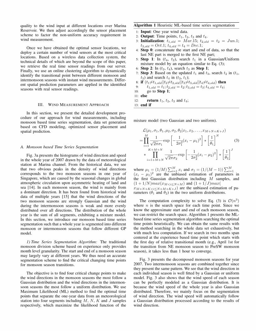
(a) Land (W10) (b) Floating (W2) (c) Mobile (6)

Fig. 12: Three types of wind sensors.

provided in the data logger and the readings of all wind sensorsare instantly synchronized in-field. A solar panel is equippedon each wind sensor to provide continuous power to the windanemometer and data logger.

Fig. 12 depicts the wind sensors that we construct in thisstudy. A land based sensor as depicted in Fig. 12a is fixedon the ground with an absolute reference direction. A floatingsensor (Fig. 12b) is anchored to the bottom of the water butfloats on the water surface. It has limited rotational freedom.We add a compass of high accuracy for each floating sensorto determine the instant reference direction which will be usedto calculate the absolute wind direction by offsetting the rawmeasurement. We also build a mobile wind sensor, as depictedin Fig. 12c. It can be easily moved and set up temporarilyat an arbitrary location. We use the mobile sensor to collectwind data for performance evaluation. Instead of solar panel,a portable battery is used to provide energy. All the othercomponents are the same as other permanent wind sensors.

B. Experiment Setup

We evaluate the performance of the proposed approach byreal measurements. With the deployed wireless wind sensornetwork, we have collected the wind data since July 2013.We study the accuracy of spatial prediction with reference ofUniGau and linear interpolation. The latter method is widelyused by current environmental analysis.

The performance gain of our proposed approach comesfrom two aspects: optimal sensor placement and accurate spa-tial prediction. Spatial prediction is based on sensor placementand they share the same system model. Since the advantagesof Gaussian-based sensor placement over random deploymenthave completely proved in previous works [5, 6] and it is costlyin terms of budget and time (more than 3 months) to reinstallsensors, we focus on evaluating the potential improvementof spatial prediction accuracy by comparing our approach(MIX) with UniGau and Interpolation. The prediction error ismeasured by the average Root-Mean-Squared Error (RMSE)between the estimated values of unobserved locations XV\Aand their actual values XV\A.

RMSE(XV\A|XA) =1

T

T∑t=1

√∑Ni∈V\A(X

ti −Xt

i )2

N(8)

Assume we have T sets of samples to conduct the evaluationand N locations are included in V\A. The result is the average

0 500 1000 15000

50

100

150

200

250

300

350

Time (minute)

Win

d di

rect

ion

(deg

ree)

Original sensor readingsMoving average

(a) Direction

0 500 1000 15000

1

2

3

4

5

6

7

8

9

Time (minute)

Win

d sp

eed

(m/s

)

Original sensor readingsMoving average

(b) Speed

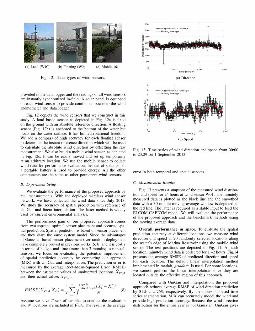
Fig. 13: Time series of wind direction and speed from 00:00to 23:29 on 1 September 2013

error in both temporal and spatial aspects.

C. Measurement Results

Fig. 13 presents a snapshot of the measured wind distribu-tion and speed for 24 hours at wind sensor W01. The minutelymeasured data is plotted as the black line and the smootheddata with a 30 minute moving average window is depicted asthe red line. The latter is required as a stable input to feed theELCOM-CAEDYM model. We will evaluate the performanceof the proposed approach and the benchmark methods usingthe moving average data.

Overall performance in space. To evaluate the spatialprediction accuracy at different locations, we measure winddirection and speed at 20 randomly selected locations alongthe water’s edge of Marina Reservoir using the mobile windsensor. The test positions are depicted in Fig. 11. At eachlocation, minutely wind data is collected for 1∼2 hours. Fig.14presents the average RMSE of predicted direction and speedfor each location. The default linear interpolation methodimplemented in matlab, griddata, is used. For some locations,we cannot perform the linear interpolation since they arelocated outside the effective region of this approach.

Compared with UniGau and interpolation, the proposedapproach reduces average RMSE of wind direction predictionby 81% and 26% respectively. By the monsoon based timeseries segmentation, MIX can accurately model the wind andprovide high prediction accuracy. Because the wind directiondistribution for the entire year is not Gaussian, UniGau gives

0 5 10 15 200

20

40

60

80

100

Test position

RM

SE

of d

irect

ion

(deg

ree)

MIXUniGauInterpolation

(a) Direction

0 5 10 15 200

0.2

0.4

0.6

0.8

1

Test position

RM

SE

of s

peed

(m

/s)

MIXUniGauInterpolation

(b) Speed

Fig. 14: Average prediction RMSE of wind direction and speedfor 20 test positions

large errors. The average RMSE of interpolation is relativelarge because it does not consider the effect of surroundingbuildings to wind field and thus cannot accurately capturethe spatial variation of wind distribution. For wind speedprediction, the performance of MIX and UniGau is comparablesince the wind speed of whole year is still Gaussian. Theyreduce the average RMSE of Interpolation by 26%. FromFig.14, we can also see that the average RMSE of locationsnear installed sensors or in open space is relatively small,because the wind patterns can be better captured by the statisticmodels and CFD modeling.

Overall performance in time. To further investigate theperformance of proposed approach for long term wind mea-surement, we use the measurement data of all 10 sensors forthree months. At one time, we choose one sensor and usethe measurement data from the rest 9 sensors to predict itswind direction and speed. We use its own measurement as thereference to calculate RMSE. We perform this evaluation in10 rounds for all 10 sensors. We do not have data from W09since it was missing a short time after installation. We areredeploying it to the opposite edge of the Kallang river whichis more secure and provides the same level of information.

Fig.15 presents the cumulative distribution of the absolutedifference between predicted observation and the measuredvalue for each sample. In this case, T and N in Eq. (8)

0 50 100 150 200 250 3000

0.1

0.2

0.3

0.4

0.5

0.6

0.7

0.8

0.9

1

Direction prediction error (degree)

CD

F

MIXUniGauInterpolation

(a) Direction

0 1 2 3 4 50

0.1

0.2

0.3

0.4

0.5

0.6

0.7

0.8

0.9

1

Speed prediction error (m/s)

CD

F

MIXUniGauInterpolation

(b) Speed

Fig. 15: Prediction error of wind direction and speed validatedby the installed wind sensors

are both equal to one. Similar to the results of the mobilesensor testing, MIX improves the prediction accuracy of winddirection by 87% for UniGau and 27% for Interpolation, andthe performances of MIX and UniGau for speed prediction arecomparable and 21% higher than that of Interpolation. MIXoffers an average spatial prediction accuracy of 24◦. The erroris larger than the mobile test since the data of one installedwind sensor is used as the reference for evaluation but notincluded in the calculation of spatial prediction.

Sensitivity of water quality. We take into account waterquality while solving the sensor placement problem so as toobtain an intended error distribution in space. Fig.16 presentsthe average RMSE at each test position in the experiment withthe mobile sensor corresponding to the sensitivity of waterquality at that location. The results show that the averageRMSE is relatively low at locations with high water qualitysensitivity. The linear regression between the water qualitysensitivities and the relative RMSEs of predicted direction fordifferent locations reveals such an inverse trend.

Online clustering algorithm. We use historical data toevaluate the efficiency of our online clustering algorithm.The experiments are done using the historical wind data ofMarina Channel meteorological station over the year 2008.The likelihood calculated by the online clustering algorithmis the average likelihood of all N samples in the sliding

5 10 15 200

1

2

3

4

5

6

7

8

RMSE of direction (degree)

Wat

er q

ualit

y se

nsiti

vity

Fig. 16: The RMSE of direction prediction corresponding tothe water quality sensitivity for each mobile test location. Thered line is the linear fitting curve of the scatter points.

Mar.1 Mar.11 Mar.21 Mar.31 Apr.10 Apr.20 Apr.30−5.7

−5.6

−5.5

−5.4

Like

lihoo

d ca

lcul

ated

onl

ine

−2.77

−2.76

−2.75

−2.74x 106

Like

lihoo

d ca

lcul

ated

offl

ine

Likelihood calculated onlineLikelihood calculated offline

Fig. 17: Likelihood calculated online and offline.

window. Only the last N samples before the time pointunder consideration are used in the calculation. We set thesliding window size N to 1440 samples corresponding to oneday and the likelihood threshold τ to 5.45. The likelihoodcalculated offline is obtained using the monsoon based timeseries segmentation algorithm introduced in Section III-A withthe whole year data. It is the sum likelihood of all samples.Fig.17 shows that the likelihoods calculated online and offlinepeak almost at the same time point for the transition from NEmonsoon season to PreSW intermonsoon season. The onlinetemporal clustering algorithm can find the critical change pointof time series with a small error of 3.6 days in this case.

V. LESSONS LEARNT

The wind we measure in this study exhibits distinct non-Gaussian process from previously studied phenomena. Besides,no full prior-knowledge is possessed to model the spatialcorrelation in the field. To work with these challenges, wetherefore developed a unique sensor placement approach in-cluding monsoon based time series segmentation and the dataset generate using CFD modeling.

The proposed approach, on the other hand, demonstrates acomplete procedure which extends the state-of-the-art sensorplacement and spatial prediction methodology to solve a wider

range of applications. There are many other phenomena whichexhibit similar non-Gaussian process captured by a mixturemodel over time, e.g., city traffic flow [16], soil pollutant [17],etc. Generalizing the time series segmentation approach in suchapplications will significantly improve the accuracy of sensorplacement and spatial prediction over clustered time periods.

Incorporating computational simulation, e.g., CFD in thiswork, to build a data set and study the field data correlationprovides us a new thought to gain prior-knowledge when intru-sive way of learning such knowledge is not preferred. We donot need to run the time-consuming computational simulationsonline, but just conduct enough simulations to cover most casesand capture the statistical features of the target phenomena.In many applications in which it is impractical to pre-deployenough sensors due to various constraints, computational sim-ulation procedure can provide coarse yet sufficient knowledgeto statistically capture the spatial correlations that we need.

VI. RELATED WORKS

The optimal sensor placement problem has been addressedin many previous works [18–20]. Among them, GP basedapproaches [8–10] have been used in many applicationsmonitoring spatial phenomena like temperature [5] and soilmoisture [6]. However, they cannot be directly applied towind distribution measurement due to the temporal and spatialvariations of wind.

The coverage problem of sensor networks has been exten-sively studied [21–23]. However, most of the existing theo-retical works are based on the deterministic disc model. Datafusion is considered in [24, 25]. The coverage and connectivityin duty-cycled sensor network are analyzed in [26–28].

CFD modeling is a widely used tool to capture the fluidpatterns in many applications, such as environmental engi-neering and aircraft design [13]. In [29], CFD has beensuccessfully applied for geospatial risk assessment of windchannels in urban area with high accuracy. CFD modelinghas also been used in sensor placement problem [30] andtemperature forecasting [31] in data center environment. CFDmodels are built to capture extra hot spot scenarios. A thermalforecasting model is proposed in [32] to model and predicttemperatures around servers in data center based on principlesfrom thermodynamics and fluid mechanics.

The time series segmentation algorithms [33, 34] searchfor critical change points by iteratively dividing data intosmall segments with the same statistical model (e.g., Gaussiandistribution). However, they cannot be applied for our mixturemodel of different statistic models, i.e., Gaussian and Uniform.Expectation Maximum algorithms [35] are utilized widely todivide a Gaussian mixture into individual Gaussian distribu-tions. However, they cannot be used in the application ofwind measurement either. First, the spatial correlation cannotbe calculated since the samples of all locations at a giventime point are not clustered in the same cluster. Second, thesamples in the same cluster are not continuous in time. As aconsequence, it is difficult to assign the online sensor readingsto a proper cluster and apply the relative spatial prediction.

VII. CONCLUSIONS

In this paper, we propose a novel sensor placement and spa-tial prediction approach for wind distribution measurements.It leverages the monsoon characteristics of wind to study itsstatistic properties. A data set is built using CFD modelingwhich captures the impact of surrounding buildings on winddistribution. Optimal sensor locations are selected throughsegmented wind statistical models and adjusted according tothe sensitivity of water quality to wind at different locations.We deployed 10 wind sensors around or on the water surface ofan urban reservoir. The observations of unobserved locationsare predicted by the readings of deployed sensors clusteredthrough an online algorithm. The in-field measurement resultsshow that the proposed approach can significantly improve theaccuracy of wind measurements.

We believe the proposed solution best exploits the under-lying nature of wind measurement in our study and achievesoptimal accuracy with a limited number of sensors. Such aprocedure nevertheless can be generalized to handle otherapplications in observing phenomenon of similar nature.

ACKNOWLEDGMENTS

This work is supported by the Singapore National Re-search Foundation under its Environmental & Water Tech-nologies Strategic Research Programmes and administeredby the Environment & Water Industry Programme Office(EWI), under project 1002-IRIS-09, Singapore MOE AcRFTier 2 MOE2012-T2-1-070, and the NTU Nanyang AssistantProfessorship (NAP) grant M4080738.020.

REFERENCES

[1] R. Alexander and J. Imberger, “Spatial distribution of motilephytoplankton in a stratified reservoir: the physical controls onpatch formation,” Journal of plankton research, 2009.

[2] Z. Xing, D. A. Fong, E. Y.-M. Lo, and S. G. Monismith, “Ther-mal structure and variability of a shallow tropical reservoir,”Limnology and Oceanography, 2014.

[3] B. Laval, J. Imberger, B. R. Hodges, and R. Stocker, “Modelingcirculation in lakes: Spatial and temporal variations,” Limnologyand Oceanography, 2003.

[4] Z. Xing, C. Liu, L. H. C. Chua, B. He, and J. Imberger,“Impacts of variable wind forcing in urban reservoirs,” in the7thInternational Symposium on Environmental Hydraulics, 2014.

[5] A. Krause, C. Guestrin, A. Gupta, and J. Kleinberg, “Near-optimal sensor placements: Maximizing information while min-imizing communication cost,” in ACM/IEEE IPSN, 2006.

[6] X. Wu, M. Liu, and Y. Wu, “In-situ soil moisture sensing:Optimal sensor placement and field estimation,” ACM Trans.Senor Networks, 2012.

[7] N. Cressie, Statistics for spatial data. John Wiley and Sons,Inc, 1993.

[8] A. Das and D. Kempe, “Sensor selection for minimizing worst-case prediction error,” in ACM/IEEE IPSN, 2008.

[9] C. Guestrin, A. Krause, and A. P. Singh, “Near-optimal sensorplacements in gaussian processes,” in ICML, 2005.

[10] M. A. Osborne, S. J. Roberts, A. Rogers, S. D. Ramchurn, andN. R. Jennings, “Towards real-time information processing ofsensor network data using computationally efficient multi-outputgaussian processes,” in ACM/IEEE IPSN, 2008.

[11] A. Krause, E. Horvitz, A. Kansal, and F. Zhao, “Towardcommunity sensing,” in ACM/IEEE IPSN, 2008.

[12] T. Burton, N. Jenkins, D. Sharpe, and E. Bossanyi, Wind energyhandbook. John Wiley & Sons, 2011.

[13] J. D. Anderson et al., Computational fluid dynamics: the basicswith applications. McGraw-Hill New York, 1995.

[14] K. E. Trenberth, D. P. Stepaniak, and J. M. Caron, “The globalmonsoon as seen through the divergent atmospheric circulation,”Journal of Climate, 2000.

[15] L. S. Chia, A. Rahman, and D. B. H. Tay, The biophysicalenvironment of Singapore. Singapore University Press, 1991.

[16] S. Sun, C. Zhang, and G. Yu, “A bayesian network approachto traffic flow forecasting,” IEEE Transactions on IntelligentTransportation Systems, 2006.

[17] Y.-P. Lin, B.-Y. Cheng, G.-S. Shyu, and T.-K. Chang, “Combin-ing a finite mixture distribution model with indicator kriging todelineate and map the spatial patterns of soil heavy metal pollu-tion in chunghua county, central taiwan,” Elsevier EnvironmentalPollution, 2010.

[18] S. S. Dhillon and K. Chakrabarty, “Sensor placement for effec-tive coverage and surveillance in distributed sensor networks,”in IEEE WCNC, 2003.

[19] F. Y. Lin and P.-L. Chiu, “A near-optimal sensor placementalgorithm to achieve complete coverage-discrimination in sensornetworks,” IEEE Communications Letters, 2005.

[20] S. Joshi and S. Boyd, “Sensor selection via convex optimiza-tion,” IEEE Transactions on Signal Processing, 2009.

[21] S. Kumar, T. H. Lai, and J. Balogh, “On k-coverage in a mostlysleeping sensor network,” in ACM MobiCom, 2004.

[22] T. Yan, Y. Gu, T. He, and J. A. Stankovic, “Design andoptimization of distributed sensing coverage in wireless sensornetworks,” ACM Transactions on Embedded Computing Sys-tems, 2008.

[23] J. Chen, J. Li, S. He, T. He, Y. Gu, and Y. Sun, “On energy-efficient trap coverage in wireless sensor networks,” ACM Trans-actions on Sensor Networks, 2013.

[24] G. Xing, C. Lu, R. Pless, and J. A. O’Sullivan, “Co-grid: anefficient coverage maintenance protocol for distributed sensornetworks,” in ACM/IEEE IPSN, 2004.

[25] G. Xing, R. Tan, B. Liu, J. Wang, X. Jia, and C.-W. Yi, “Datafusion improves the coverage of wireless sensor networks,” inACM MobiCom, 2009.

[26] X. Wang, G. Xing, Y. Zhang, C. Lu, R. Pless, and C. Gill,“Integrated coverage and connectivity configuration in wirelesssensor networks,” in ACM SenSys, 2003.

[27] Y. Gu, L. Cheng, J. Niu, T. He, and D. H. Du, “Achievingasymmetric sensing coverage for duty cycled wireless sensornetworks,” IEEE Transactions on Parallel and Distributed Sys-tems, 2013.

[28] T. Yan, T. He, and J. A. Stankovic, “Differentiated surveillancefor sensor networks,” in ACM SenSys, 2003.

[29] T. K. Lim, H. Miao, C. Chew, K. K. Lee, and D. K. Raju,“Environmental modeling for geospatial risk assessment of windchannels in singapore,” in GSDI, 2012.

[30] X. Wang, X. Wang, G. Xing, J. Chen, C.-X. Lin, and Y. Chen,“Towards optimal sensor placement for hot server detection indata centers,” in IEEE ICDCS, 2011.

[31] J. Chen, R. Tan, Y. Wang, G. Xing, X. Wang, X. Wang,B. Punch, and D. Colbry, “A high-fidelity temperature distribu-tion forecasting system for data centers,” in IEEE RTSS, 2012.

[32] L. Li, C.-J. M. Liang, J. Liu, S. Nath, A. Terzis, and C. Falout-sos, “Thermocast: a cyber-physical forecasting model for data-centers.” in ACM KDD, 2011.

[33] P. Bernaola-Galvan, R. Roman-Roldan, and J. L. Oliver, “Com-positional segmentation and long-range fractal correlations indna sequences,” Physical Review E, 1996.

[34] V. Guralnik and J. Srivastava, “Event detection from time seriesdata,” in ACM KDD, 1999.

[35] A. P. Dempster, N. M. Laird, and D. B. Rubin, “Maximumlikelihood from incomplete data via the EM algorithm,” Journalof the Royal Statistical Society. Series B (Methodological), 1977.