optimal searching - home page | mit csail · optimal searching best-first search review •...

1

Optimal searching

Best-first search review

• Advantages– Takes advantage of domain information to guide search– Greedy advance to the goal

• Disadvantages– Considers cost to the goal from the current state– Some path can continue to look good according to the

heuristic function3 2

1

x

1 1 1 xAt this point the path is morecostly than the alternate path

2

Branch & Bound

• Use current cost (past cost) to a node• Pick best (lowest) cost.• If f is our evaluation function for node n,

f(n)= g(n) [g= cost ‘gone so far’g ≥ 0

• B&B: sort queue in order of lowest f, & make sure not to pursue identical paths with higher costs than known costs

The A* Algorithm:combining past with future

• Now Consider the overall cost of the solution.

f(n) = g(n) + h(n) where g(n) is the path cost to node g= distance gone so far h= future estimated costthink of f(n) as an estimate of the cost of the best solution going

through the node n

3 3

2

x

3 4 5 x

3 2

1

x

1 1 1 x

3

UCS, BFS, Best-First, and A*

• f = g + h A* Search• h = 0 Uniform cost search• g = 1, h = 0 Breadth-First search• g = 0 Best-First search

Admissible Heuristics

• This is not quite enough, we also require h be admissible: – a heuristic h is admissible if h(n) < h*(n) for all nodes n, – where h* is the actual cost of the optimal path from n to the

goal

• Examples: – travel distance straight line distance must be shorter than

actual travel path – tiles out of place each move can reorder at most one tile

distance of each out of place tile from the correct place each move moves a tile at most one place toward correct place

4

Heuristic Functions

• Tic-tac-toe

xx

x

o xxxxx o

oo o

xxx

ooo

8 Puzzle

• Exhaustive Search : 3 20 = 3 * 10 9states

• Remove repeated state : 9! = 362,880• Use of heuristics

– h1 : # of tiles that are in the wrong position– h2 : sum of Manhattan distance

h1 = 3

h2 = 1+2+2=547658321

56748321

5

Heuristics : 8 Puzzle

47658321

45768321

47658321

56748321

47658321

Tic-tac-toe

• Most-Win Heuristics

x x

x

3 win 4 win 2 win

6

Road Map Problem

s

g

h(s)

n

h(n)

n’h(n’)

g(n’)

Effect of Heuristic Accuracy on Performance

• Well-designed heuristic have its branch close to 1• h2 dominates h1 iff

h2(n) ≥ h1(n), ∀ n• It is always better to use a heuristic function with

higher values, as long as it does not overestimate• Inventing heuristic functions

– Cost of an exact solution to a relaxed problem is a good heuristic for the original problem

– collection of admissible heuristicsh*(n) = max(h1(n), h2(n), …, hk(n))

7

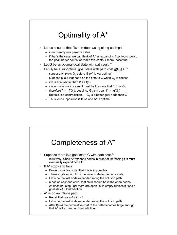
Optimality of A*• Let us assume that f is non-decreasing along each path

– if not, simply use parent’s value – if that’s the case, we can think of A* as expanding f contours toward

the goal; better heuristics make this contour more “eccentric”• Let G be an optimal goal state with path cost f*• Let G2 be a suboptimal goal state with path cost g(G2) > f*.

– suppose A* picks G2 before G (A* is not optimal) – suppose n is a leaf node on the path to G when G2 is chosen – if h is admissible, then f* >= f(n) – since n was not chosen, it must be the case that f(n) >= G2

– therefore f* >= f(G2), but since G2 is a goal, f* >= g(G2) – But this is a contradiction --- G2 is a better goal node than G – Thus, our supposition is false and A* is optimal.

Completeness of A*• Suppose there is a goal state G with path cost f*

– Intuitively: since A* expands nodes in order of increasing f, it must eventually expand node G

• If A* stops and fails– Prove by contradiction that this is impossible.– There exists a path from the initial state to the node state – Let n be the last node expanded along the solution path– n has at least one child, that child should be in the open nodes– A* does not stop until there are open list is empty (unless it finds a

goal state). Contradiction.• A* is on an infinite path

– Recall that cost(s1,s2) > δ– Let n be the last node expanded along the solution path– After f(n)/δ the cumulative cost of the path becomes large enough

that A* will expand n. Contradiction.

8

Properties of A*Properties of A*• Suppose C* is the cost of the optimal solution path

– A* expands all nodes with f(n) < C*– A* might expand some of nodes with f(n) = C* on the

“goal contour”– A* will expand no nodes with f(n) > C*, which are pruned!– Pruning: eliminating possibilities from consideration

without examination

• A* is optimally efficient for any given heuristic function– no other optimal algorithm is guaranteed to expand fewer

nodes than A*– an algorithm might miss the optimal solution if it does not

expand all nodes with f(n) < C*

• A* is complete

9

A* summary

• Completeness – provided finite branching factor and finite cost per operator

• Optimality– provided we use an admissible heuristic

• Time complexity – worst case is still O(bd) in some special cases we can do

better for a given heuristic

• Space complexity – worst case is still O(bd)

Finding heuristics: Relax Optimality (note: this is not required material)

• Goals:– Minimizing search cost– Satisficing solution, i.e. bounded error in the

solutionf(s) = (1-w) g(s) + w h(s)

– g can be thought of as the breadth first component– w = 1 => Best-First search– w = .5 => A* search– w = 0 => Uniform search

10

Iterative Deepening A*

• Goals– A storage efficient algorithm that we can use in practice– Still complete and optimal

• Modification of A*– use f-cost limit as depth bound

– increase threshold as minimum of f(.) of previous cycle• Each iteration expands all nodes inside the contour

for current f-cost• same order of node expansion

Games

• Why games?– Games provide an environment of pure competition with

objective goals between agents. – Game playing is considered an intelligent human activity.– The environment is deterministic and accessible.– The set of operators is small and defined.– Large state space– Fun!

11

Games• Consider Games

– Two player games– Perfect Information: not involving chance or hidden

information (not back-gammon, poker)– Zero-sum games: games where our gain is our opponents

loss– Examples: tic-tac-toe, checkers, chess, go

• Games of perfect information are really just search problems– initial state– operators to generate new states– goal test– utility function (win/lose/draw)

Game Trees

• Tic-tac-toe

xx

x

o xxxxx o

oo o

xxx

ooo

1 ply 1 move

12

Game Trees Examplewin

lose

draw

xxo

o

ox

xxo

o

ox

xxo

o

oxx

xxo

o

ox

x x

xxo

o

oxx

xxo

o

oxx

xxo

o

ox

x

xxo

o

ox

x

xxo

o

ox

x

xxo

o

ox

xo

oo oo

o

xxo

o

oxx

o x xxx

xxo

o

oxx

o

xxo

o

ox

xo

xxo

o

ox

xo x

xxo

o

ox

xo

What’s a good move?win

lose

draw

xxo

o

ox

xxo

o

ox

xxo

o

oxx

xxo

o

ox

x x

xxo

o

oxx

xxo

o

oxx

xxo

o

ox

x

xxo

o

ox

x

xxo

o

ox

x

xxo

o

ox

xo

oo oo

o

xxo

o

oxx

o x xxx

xxo

o

oxx

o

xxo

o

ox

xo

xxo

o

ox

xo x

xxo

o

ox

xo

13

Game Trees Examplewin

lose

draw

xxo

o

ox

xxo

o

ox

xxo

o

oxx

xxo

o

ox

x x

xxo

o

oxx

xxo

o

oxx

xxo

o

ox

x

xxo

o

ox

x

xxo

o

ox

x

xxo

o

ox

xo

oo oo

o

xxo

o

oxx

o x xxx

xxo

o

oxx

o

xxo

o

ox

xo

xxo

o

ox

xo x

xxo

o

ox

xo

Perfect decisions in 2-person games

Let’s name the two agents (players) MAX and MIN• MAX is searching for the highest utility state, so when

it is MAX’s move she will maximize the payoff• High utility for MAX is low utility for MIN, since it’s a

zero-sum game• When it is MIN’s move she will minimize the payoff• The winning strategy is to maximize over minimum

payoff moves.

14

Minimax Algorithm

For the MAX player1. Generate the game to terminal states2. Apply the utility function to the terminal

states3. Back-up values

• At MIN ply assign minimum payoff move• At MAX ply assign maximum payoff move

4. At root, MAX chooses the operator that led to the highest payoff

Minimax ExampleTwo-ply game

Max

Min

Max

A11 A12A13

A21A22 A23

A31

A32 A33

A1 A2 A3

15


Max

Min

Max

A11 A12A13

A21A22 A23

A31

A32 A33

A1 A2 A3

3 12 8 2 4 6 14 5 2


Max

Min

Max

A11 A12A13

A21A22 A23

A31

A32 A33

A1 A2 A3

3 12 8 2 4 6 14 5 2

3 2 2

16


Max

Min

Max

A11 A12A13

A21A22 A23

A31

A32 A33

A1 A2 A3

3 12 8 2 4 6 14 5 2

3 2 2

3

Minimax

• Perfect play for deterministic, perfect-information games

• Totally impractical since it generates the whole tree– Time complexity is O(bd)!– Space complexity is O(bd)

17

The Complexity of Minimax

• For a given game with branching factor b, searching to depth d require O(bd) computation and storage– chess has a branching factor of around 35

• A 1-move search tree for chess has 1225 leaves• Say a typical chess game has 100 moves then the

number of leaves in the tree is 35100 = 10154

• Assuming a modern computer can process 1000000 board positions a second it will take 10140 years to search the entire tree.

– go has a branching factor of 360 or more

Partial Search Tree

• In a real game, we can only look ahead a few ply!• The depth of search is determined by the time

allowed per move.• Suppose we can process 1000000 positions a

second and we’re allowed one minute per move, then we can search 5 ply.

35

1225

42875

1500625

52521875

18

Minimax Cutoff

• Does it work in practice?– Time complexity: O(bm)

• Chess:– b = 35– Suppose we limit our search to 1.5 million nodes

per move– m = 4– 4-ply chess player is a lousy player!– 4-ply = novice chess player– 8-ply = typical PC, human master– 12-ply = Deep Blue, Kasparov

The Evaluation Function

• If we do not reach the end of the game how do we evaluate the payoff of the leaf states?

• Use a static evaluation function. – A heuristic function that estimates the utility of board positions.– Desirable properties

• Must agree with the utility function• Must not take too long to evaluate• Must accurately reflect the chance of winning

• An ideal evaluation function can be applied directly to the board position.

• It is better to apply it as many levels down in the game tree astime permits.

• Example evaluation functions:– Tic-Tac-Toe: # ways to win– Chess: value of white pieces/value of black pieces

19

Minimax

o

xx

x

o xxxxx oo o

xxx

ooo

2 2 3 2 2 2 2 2

xo

1

xo

3

# ways to win heuristic

Minimax

o

xx

x

o xxxxx oo o

xxx

ooo

2 2 3 2 2 2 2 2

xo

1

xo

3

2 21

20

Minimax

o

xx

x

o xxxxx oo o

xxx

ooo

2 2 3 2 2 2 2 2

xo

1

xo

3

2 21

2

Revised Minimax Algorithm

For the MAX player1. Generate the game as deep as time permits2. Apply the evaluation function to the leaf states3. Back-up values

• At MIN ply assign minimum payoff move• At MAX ply assign maximum payoff move

4. At root, MAX chooses the operator that led to the highest payoff

21

Cutting Off Search

• Because the evaluation function is only an approximation it can misguide us.– Example: white appears to have the

advantage, but black captures the queen in the next move. Need to search one more ply

• Often, it makes sense to make depth dynamically decided

• quiescence search --- go until things seem stable– Example: in chess, don’t stop in positions

where capture moves are imminent

Nonquiescent

The Horizon Problem

• When a move by the opponent causes serious damage, but is ultimately unavoidable.– Example: the pawn on the 7th row will

be queened eventually.

• The problem: the player can push this event off beyond the search horizon

• No known solution to the horizon problem.

22

Alpha-beta Pruning• Efficiency hack on top of minimax: gets same result,

but fewer evaluations • Basic idea: keep track of your best move's value so

far while performing minimax search• For Max, that value is called alpha

– When Min is examining its moves, and it gets one back that is less than alpha (i.e., worse for Max), then its parent, Max, would not make that move because the move that gave alpha is better. So Min can abandon this node right now before examining any more moves from it

• Ditto for Min, but the best value so far is called beta (Min wants to make beta as small as possible)– When Max is expanding its moves, if any are greater than

beta (i.e., worse for Min) than it can stop early• Starts with worst possible alpha (negative

infinity) and beta (positive infinity)

Alpha-Beta Pruning ExampleTwo-ply game

Max

Min

Max

3 12 8

3

-∞

23


Max

Min

Max

3 12 8

3

≥ 3


Max

Min

Max

3 12 8

3

2

X X

≥ 3

≤ 2

When Min is examining its moves, and it gets oneback that is less than alpha (i.e., worse for Max),

then its parent, Max, would not make that movebecause the move that gave alpha is better.

So Min can abandon this node right now beforeexamining any more moves from it

24


Max

Min

Max

3 12 8

3

2

X X

≥ 3

≤ 2

14

≤ 14


Max

Min

Max

3 12 8

3

2

X X

≥ 3

≤ 2

14

≤ 14

5

25


Max

Min

Max

3 12 8

3

2

X X

≥ 3

≤ 2

14

≤ 14 5

5

X


Max

Min

Max

3 12 8

3

2

X X

≥ 3

≤ 2

14

≤ 14 5

5

X

2

X X

26


Max

Min

Max

3 12 8

3

2

X X

≥ 3

≤ 2

14

≤ 14 5 2

5

X

2

X X

X


Max

Min

Max

3 12 8

3

2

X X

≥ 3

≤ 2

14

≤ 14 5 2

5

X

2

X X

X

27


Max

Min

Max

3 12 8

3

2

X X

3

≤ 2

14

≤ 14 5 2

5

X

2

X X

X

Alpha-beta pruning

• Pruning does not affect final result• Alpha-beta pruning

– Good move ordering improves effectiveness of pruning

– Asymptotic time complexity• O((b/log b)d)

– With “perfect ordering,” time complexity• O(bd/2)• means we go from an effective branching factor of b to

sqrt(b) (e.g. 35 -> 6).

28

Complexity of Alpha-Beta Pruning

• Order the nodes so that best moves for that player are investigated first– tend to get alpha and beta to optimal values faster– so get more pruning

• If a decent heuristic for ordering moves can be found--– Time complexity approaches O(b^(d/2))

• If moves are randomly ordered, then around O(b^(3d/4)) • But these both assume randomly distributed utilities

– need empirical work with real games• Space complexity is O(bd)

– The same as other depth-first searches

From here on is optional material

29

α−β Procedure pseudo-codeminimax-α−β(board, depth, type, α, β)

If depth = 0 return Eval-Fn(board)else if type = max

cur-max = -infloop for b in succ(board)

b-val = minimax-α−β(b,depth-1,min, α, β)cur-max = max(b-val,cur-max)α = max(cur-max, α)if cur-max >= β finish loop

return cur-maxelse (type = min)

cur-min = infloop for b in succ(board)

b-val = minimax-α−β(b,depth-1,max, α, β)cur-min = min(b-val,cur-min)β = min(cur-min, β)if cur-min <= α finish loop

return cur-min

Games That Include an Element of Chance

• Many games mirror unpredictability by including a random element

• E.g. backgammon

30

Game tree for a backgammon

Decision Making in Game of Chance

• Chance nodes– Branches leading from each chance node denote

the possible dice rolls– Labeled with the roll and the chance that it will

occur• Replace MAX/MIN nodes in minimax with

expected MAX/MIN payoff– Expectimax value of C

– Expectimin value))((max)()( ),( sutilitydPCexpectimax idCS

isi ∈∑=

))((min)()( ),( sutilitydPCexpectimin idCSi

si ∈∑=

31

Position evaluation in games with chance nodes

• For minimax, any order-preserving transformation of the leaf values does not affect the choice of move

• With chance node, some order-preserving transformations of the leaf values do affect the choice of move

Position evaluation in games with chance nodes (cont’d)

⇒ The behavior of the algorithm is sensitive even to a linear transformation of the evaluation function.

32

Complexity of expectiminimax

• The expectiminimax considers all the possible dice-roll sequences– It takes O(bmnm)

where n is the number of distinct rolls– Whereas, minimax takes O(bm)

• Problems– The extra cost compared to minimax is very high– Alpha-beta pruning is more difficult to apply

State-of-the-Art for Chess Programs

• Chess basics– 8x8 board, 16 pieces per side, average branching

factor of about 35– Rating system based on competition

• 500 --- beginner/legal• 1200 --- good weekend warrior• 2000 --- world championship level• 2500+ --- grand master

– time limited moves– open and closing books available– important aspects: position, material

33

Chess Ratings

Sketch of Chess History

• First discussed by Shannon, Sci. American, 1950• Initially, two approaches

– human-like– brute force search

• 1966 MacHack ---1100 --- average tournament player• 1970’s

– discovery that 1 ply = 200 rating points– hash tables– quiescence search

• Chess 4.x reaches 2000 (expert level), 1979• Belle 2200, 1983

– special purpose hardware• 1986 --- Cray Blitz and Hitech 100,000 to 120,000 position/sec

using special purpose hardware

34

IBM checks in

• Deep thought:– 250 chips (2M pos/sec /// 6-7M pos/soc)– Evaluation hardware

• piece placement• pawn placement• passed pawn eval• file configurations• 120 parameters to tune

– Tuning done to master’s games• hill climbing and linear fits

– 1989 --- rating of 2480 === Kasparov beats

IBM Ups the Ante• Deep Blue is the next generation

– parallel version of deep thought– 200 M pos/sec 60B positions in the 3 minutes allotted for move– DB 1 = 32 Rs/6000’s with 6 chess proc/node– DB 2 = faster 32 nodes w 8 chess proc/node (256 proc)– message passing architecture– search as much as 20-30 levels deep using sing. extension

• In 1997, Kasparov beaten– Kasparov changed strategy in earlier games– As much a psychological as mental victory

• http://www.research.ibm.com/deepblue/home/html/b.html

35

Chess Programs Today

• Deep Blue dismantled --- leaves void in the world of chess programs

• Deep Junior• Deep Fritz

– A commercial product– Pentium III dual processing 933 MHz computers– Analyze 6 million moves per second– As strong as Deep Blue

4==11=00=Deep Fritz4==00=11=Vladimir KramnikFinal87654321

Man vs. Machine, Bahrain, October 2002

State-of-the-art for Checkers Programs

• Checker– Arthur Samuel (1952)

– official world champion – Chinook– Uses extensive move database

36

State-of-the-art for Backgammon Programs

• Use a temporal differencing algorithm to train a neural network• Strongest Programs: TD-GAMMON by Gary Tesauro of IBM,

Jellyfish• Achieve expert level play

State-of-the-art for Othello Programs

• Programs stronger than human players• Programs use learning techniques to fine-tune the evaluation

function, the opening book, and even the search algorithm• Strongest programs: Logistello, Hannibal

37

State-of-the-art for GO Programs

• Branching factor of GO about 360• Humans lead by a huge margin• Many, many programs

– From recent Go Ladder competition: Go4++, Many Faces of Go, Ego 1, NeuroGo II, Explorer, Indigo, Golois, Gnu Go, Gobble, gottaGo, Poka, Viking, GoLife I, The Turtle, Gogo, GL7

State-of-the-art for Poker Programs

• Poki (University of Alberta) is probably the strongest poker program• Not close to world-class level

optimal searching - home page | mit csail · optimal searching best-first search review •...

Documents