optimal search trees with 2-way comparisonsneal/chrobak15optimal.pdf · optimal search trees with...

Optimal Search Trees with 2-Way Comparisons

Marek Chrobak1, Mordecai Golin2, J. Ian Munro3, and Neal E. Young1(B)

1 University of California – Riverside, Riverside, CA, [email protected]

2 Hong Kong University of Science and Technology, Hong Kong, China3 University of Waterloo, Waterloo, Canada

Abstract. In 1971, Knuth gave an O(n2)-time algorithm for the clas-sic problem of finding an optimal binary search tree. Knuth’s algorithmworks only for search trees based on 3-way comparisons, but most mod-ern computers support only 2-way comparisons (<, ≤, =, ≥, and >).Until this paper, the problem of finding an optimal search tree using 2-way comparisons remained open — poly-time algorithms were knownonly for restricted variants. We solve the general case, giving (i) anO(n4)-time algorithm and (ii) an O(n log n)-time additive-3 approxima-tion algorithm. For finding optimal binary split trees, we (iii) obtain alinear speedup and (iv) prove some previous work incorrect.

1 Background and Statement of Results

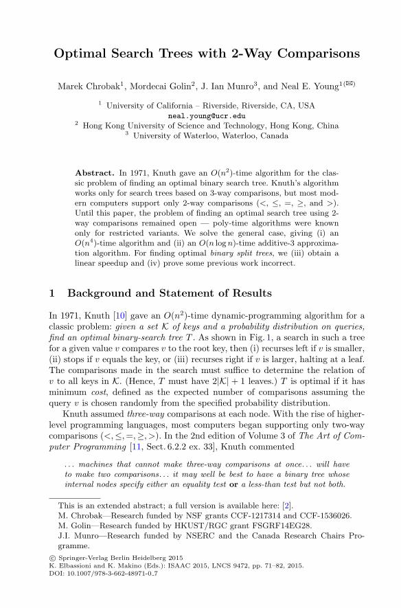
In 1971, Knuth [10] gave an O(n2)-time dynamic-programming algorithm for aclassic problem: given a set K of keys and a probability distribution on queries,find an optimal binary-search tree T . As shown in Fig. 1, a search in such a treefor a given value v compares v to the root key, then (i) recurses left if v is smaller,(ii) stops if v equals the key, or (iii) recurses right if v is larger, halting at a leaf.The comparisons made in the search must suffice to determine the relation ofv to all keys in K. (Hence, T must have 2|K| + 1 leaves.) T is optimal if it hasminimum cost, defined as the expected number of comparisons assuming thequery v is chosen randomly from the specified probability distribution.

Knuth assumed three-way comparisons at each node. With the rise of higher-level programming languages, most computers began supporting only two-waycomparisons (<,≤,=,≥, >). In the 2nd edition of Volume 3 of The Art of Com-puter Programming [11, Sect. 6.2.2 ex. 33], Knuth commented

. . . machines that cannot make three-way comparisons at once. . . will haveto make two comparisons. . . it may well be best to have a binary tree whoseinternal nodes specify either an equality test or a less-than test but not both.

This is an extended abstract; a full version is available here: [2].M. Chrobak—Research funded by NSF grants CCF-1217314 and CCF-1536026.M. Golin—Research funded by HKUST/RGC grant FSGRF14EG28.J.I. Munro—Research funded by NSERC and the Canada Research Chairs Pro-gramme.

c© Springer-Verlag Berlin Heidelberg 2015K. Elbassioni and K. Makino (Eds.): ISAAC 2015, LNCS 9472, pp. 71–82, 2015.DOI: 10.1007/978-3-662-48971-0 7

72 M. Chrobak et al.

v ? O

v ? Wv ? H< >

v=O=

< >

v=H

=H<v<Ov<H

< >v=W=

W<vO<v<W

v

Fig. 1. A binary search tree T using 3-way comparisons, for K = {H, O, W}.

v = H?v < O?

v < W?yes

y

no

ny

v=H v < H?y

v<H H<v<On

n

v = O? v = W?y

v=Wn

W<v

y

v=O O<v<Wn

vv < O?

v = O?yes

y

no

v=Hn

v=Wv=O

v(b)(a)

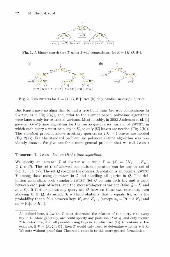
Fig. 2. Two 2wcsts for K = {H, O, W}; tree (b) only handles successful queries.

But Knuth gave no algorithm to find a tree built from two-way comparisons (a2wcst, as in Fig. 2(a)), and, prior to the current paper, poly-time algorithmswere known only for restricted variants. Most notably, in 2002 Anderson et al. [1]gave an O(n4)-time algorithm for the successful-queries variant of 2wcst, inwhich each query v must be a key in K, so only |K| leaves are needed (Fig. 2(b)).The standard problem allows arbitrary queries, so 2|K| + 1 leaves are needed(Fig. 2(a)). For the standard problem, no polynomial-time algorithm was pre-viously known. We give one for a more general problem that we call 2wcst:

Theorem 1. 2wcst has an O(n4)-time algorithm.

We specify an instance I of 2wcst as a tuple I = (K = {K1, . . . ,Kn},Q, C, α, β). The set C of allowed comparison operators can be any subset of{<,≤,=,≥, >}. The set Q specifies the queries. A solution is an optimal 2wcstT among those using operators in C and handling all queries in Q. This def-inition generalizes both standard 2wcst (let Q contain each key and a valuebetween each pair of keys), and the successful-queries variant (take Q = K andα ≡ 0). It further allows any query set Q between these two extremes, evenallowing K �⊆ Q. As usual, βi is the probability that v equals Ki; αi is theprobability that v falls between keys Ki and Ki+1 (except α0 = Pr[v < K1] andαn = Pr[v > Kn]).1

1 As defined here, a 2wcst T must determine the relation of the query v to everykey in K. More generally, one could specify any partition P of Q, and only requireT to determine, if at all possible using keys in K, which set S ∈ P contains v. Forexample, if P = {K, Q \ K}, then T would only need to determine whether v ∈ K.We note without proof that Theorem 1 extends to this more general formulation.

Optimal Search Trees with 2-Way Comparisons 73

To prove Theorem 1, we prove Spuler’s 1994 “maximum-likelihood” conjec-ture: in any optimal 2wcst tree, each equality comparison is to a key in Kof maximum likelihood, given the comparisons so far [14, Sect. 6.4 Conj. 1]. AsSpuler observed, the conjecture implies an O(n5)-time algorithm; we reduce thisto O(n4) using standard techniques and a new perturbation argument. Andersonet al. proved the conjecture for their special case [1, Cor. 3]. We were unable toextend their proof directly; our proof uses a different local-exchange argument.

We also give a fast additive-3 approximation algorithm:

Theorem 2. Given any instance I = (K,Q, C, α, β) of 2wcst, one can computea tree of cost at most the optimum plus 3, in O(n log n) time.

Comparable results were known for the successful-queries variant (Q = K) [1,16].We approximately reduce the general case to that case.

Binary split trees “split” each 3-way comparison in Knuth’s 3-way-comparisonmodel into two 2-way comparisons within the same node: an equality compari-son (which, by definition, must be to the maximum-likelihood key) and a “<”comparison (to any key) [3,6,8,12,13]. The fastest algorithms to find an opti-mal binary split tree take O(n5)-time: from 1984 for the successful-queries-onlyvariant (Q = K) [8]; from 1986 for the standard problem (Q contains queries inall possible relations to the keys in K) [6]. We obtain a linear speedup:

Theorem 3. Given any instance I = (K = {K1, . . . ,Kn}, α, β) of the standardbinary-split-tree problem, an optimal tree can be computed in O(n4) time.

The proof uses our new perturbation argument (Sect. 3.1) to reduce to the casewhen all βi’s are distinct, then applies a known algorithm [6]. The perturbationargument can also be used to simplify Anderson et al.’s algorithm [1].

Generalized binary split trees (gbsts) are binary split trees without themaximum-likelihood constraint. Huang and Wong [9] (1984) observe that relax-ing this constraint allows cheaper trees — the maximum-likelihood conjecturefails here — and propose an algorithm to find optimal gbsts. We prove it incor-rect!

Theorem 4. Lemma 4 of [9] is incorrect: there exists an instance — a querydistribution β — for which it does not hold, and on which their algorithm fails.

This flaw also invalidates two algorithms, proposed in Spuler’s thesis [15], thatare based on Huang and Wong’s algorithm. We know of no poly-time algorithmto find optimal gbsts. Of course, optimal 2wcsts are at least as good.

2wcstwithout equality tests. Finding an optimal alphabetical encoding has sev-eral poly-time algorithms: by Gilbert and Moore — O(n3) time, 1959 [5];by Hu and Tucker — O(n log n) time, 1971 [7]; and by Garsia and Wachs— O(n log n) time but simpler, 1979 [4]. The problem is equivalent to find-ing an optimal 3-way-comparison search tree when the probability of query-ing any key is zero (β ≡ 0) [11, Sect. 6.2.2]. It is also equivalent to findingan optimal 2wcst in the successful-queries variant with only “<” comparisons


allowed (C = {<},Q = K) [1, Sect. 5.2]. We generalize this observation to proveTheorem 5:

Theorem 5. Any 2wcst instance I = (K = {K1, . . . ,Kn},Q, C, α, β) where =is not in C (equality tests are not allowed), can be solved in O(n log n) time.

Definition 1. Fix any 2wcst instance I = (K,Q, C, α, β).For any node N in any 2wcst T for I, N ’s query subset, QN , contains

queries v ∈ Q such that the search for v reaches N . The weight ω(N) of N isthe probability that a random query v (from distribution (α, β)) is in QN . Theweight ω(T ′) of any subtree T ′ of T is ω(N) where N is the root of T ′.

Let 〈v < Ki〉 denote an internal node having key Ki and comparison operator< (define 〈v ≤ Ki〉 and 〈v = Ki〉 similarly). Let 〈Ki〉 denote the leaf N such thatQN = {Ki}. Abusing notation, ω(Ki) is a synonym for ω(〈Ki〉), that is, βi.

Say T is irreducible if, for every node N with parent N ′, QN �= QN ′ .

In the remainder of the paper, we assume that only comparisons in {<,≤,=}are allowed (i.e., C ⊆ {<,≤,=}). This is without loss of generality, as “v > Ki”and “v ≥ Ki” can be replaced, respectively, by “v ≤ Ki” and “v < Ki.”

2 Proof of Spuler’s Conjecture

Fix any irreducible, optimal 2wcst T for any instance I = (K,Q, C, α, β).

Theorem 6 (Spuler’s conjecture). The key Ka in any equality-comparisonnode N = 〈v = Ka〉 is a maximum-likelihood key: βa = maxi{βi : Ki ∈ QN}.The theorem will follow easily from Lemma 1:

Lemma 1. Let internal node 〈v = Ka〉 be the ancestor of internal node〈v = Kz〉. Then ω(Ka) ≥ ω(Kz). That is, βa ≥ βz.

Proof (Lemma 1). Throughout, “〈v ≺ Ki〉” denotes a node in T that does aninequality comparison (≤ or <, not =) to key Ki. Abusing notation, in thatcontext, “x ≺ Ki” (or “x �≺ Ki”) denotes that x passes (or fails) that comparison.

Assumption 1. (i) All nodes on the path from 〈v = Ka〉 to 〈v = Kz〉 doinequality comparisons. (ii) Along the path, some other node 〈v ≺ Ks〉 separateskey Ka from Kz: either Ka ≺ Ks but Kz �≺ Ks, or Kz ≺ Ks but Ka �≺ Ks.

It suffices to prove the lemma assuming (i) and (ii) above. (Indeed, if the lemmaholds given (i), then, by transitivity, the lemma holds in general. Given (i), if(ii) doesn’t hold, then exchanging the two nodes preserves correctness, changingthe cost by (ω(Ka)−ω(Kz))×d for d ≥ 1, so ω(Ka) ≥ ω(Kz) and we are done.)

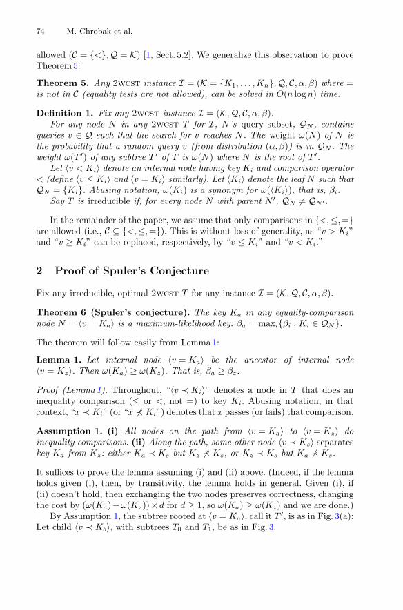
By Assumption 1, the subtree rooted at 〈v = Ka〉, call it T ′, is as in Fig. 3(a):Let child 〈v ≺ Kb〉, with subtrees T0 and T1, be as in Fig. 3.


v = Ka

v ≺ Kb

T0

Ka

(a)

T1

v = Ka

v ≺ Kb

T0Ka

T1

(b)

y n

yy n

yn

n

v = Ka

v ≺ Kb

T1Ka

T0

(c)

ny

yn

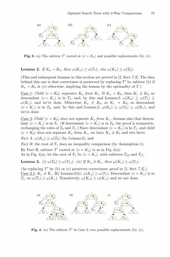
Fig. 3. (a) The subtree T ′ rooted at 〈v = Ka〉 and possible replacements (b), (c).

Lemma 2. If Ka ≺ Kb, then ω(Ka) ≥ ω(T1), else ω(Ka) ≥ ω(T0).

(This and subsequent lemmas in this section are proved in [2, Sect. 7.2]. The ideabehind this one is that correctness is preserved by replacing T ′ by subtree (b) ifKa ≺ Kb or (c) otherwise, implying the lemma by the optimality of T .)

Case 1: Child 〈v ≺ Kb〉 separates Ka from Kz. If Ka ≺ Kb, then Kz �≺ Kb, sodescendant 〈v = Kz〉 is in T1, and, by this and Lemma2, ω(Ka) ≥ ω(T1) ≥ω(Kz), and we’re done. Otherwise Ka �≺ Kb, so Kz ≺ Kb, so descendant〈v = Kz〉 is in T0, and, by this and Lemma2, ω(Ka) ≥ ω(T0) ≥ ω(Kz), andwe’re done.

Case 2: Child 〈v ≺ Kb〉 does not separate Ka from Kz. Assume also that descen-dant 〈v = Kz〉 is in T1. (If descendant 〈v = Kz〉 is in T0, the proof is symmetric,exchanging the roles of T0 and T1.) Since descendant 〈v = Kz〉 is in T1, and child〈v ≺ Kb〉 does not separate Ka from Kz, we have Ka �≺ Kb and two facts:Fact A: ω(Ka) ≥ ω(T0) (by Lemma 2), andFact B: the root of T1 does an inequality comparison (by Assumption 1).By Fact B, subtree T ′ rooted at 〈v = Ka〉 is as in Fig. 4(a):As in Fig. 4(a), let the root of T1 be 〈v ≺ Kc〉, with subtrees T10 and T11.

Lemma 3. (i) ω(T0) ≥ ω(T11). (ii) If Ka �≺ Kc, then ω(Ka) ≥ ω(T1).

(As replacing T ′ by (b) or (c) preserves correctness; proof in [2, Sect. 7.2].)Case 2.1: Ka �≺ Kc. By Lemma 3(ii), ω(Ka) ≥ ω(T1). Descendant 〈v = Kz〉 is inT1, so ω(T1) ≥ ω(Kz). Transitively, ω(Ka) ≥ ω(Kz), and we are done.

n

)b()a(

T1

v ≺ Kb

T0v ≺Kc

T10 T11

v = Ka

Ka

y

y

y

n

nv ≺Kb

T0

v ≺Kc

T10

v = Ka

T11Ka

y

y

y

n

n n y

y

n

n

(c)

v ≺Kb

T0

v ≺Kc

T10

T11

v = Ka

Ka

y

Fig. 4. (a) The subtree T ′ in Case 2, two possible replacements (b), (c).


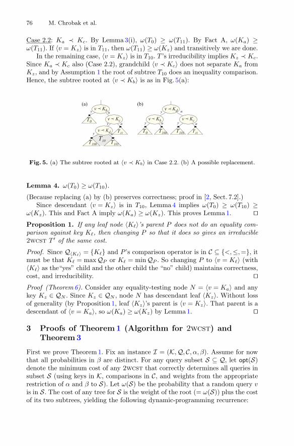
Case 2.2: Ka ≺ Kc. By Lemma 3(i), ω(T0) ≥ ω(T11). By Fact A, ω(Ka) ≥ω(T11). If 〈v = Kz〉 is in T11, then ω(T11) ≥ ω(Kz) and transitively we are done.

In the remaining case, 〈v = Kz〉 is in T10. T ’s irreducibility implies Kz ≺ Kc.Since Ka ≺ Kc also (Case 2.2), grandchild 〈v ≺ Kc〉 does not separate Ka fromKz, and by Assumption 1 the root of subtree T10 does an inequality comparison.Hence, the subtree rooted at 〈v ≺ Kb〉 is as in Fig. 5(a):

y

y

y

n

n

n

y

y yn

n

n

(a) (b)v ≺ Kb

T0 v ≺ Kc

T11

T10

v ≺ Kd

T100 T101

v ≺Kb

T0

v ≺Kc

T11

v ≺Kd

T100 T101

Fig. 5. (a) The subtree rooted at 〈v ≺ Kb〉 in Case 2.2. (b) A possible replacement.

Lemma 4. ω(T0) ≥ ω(T10).

(Because replacing (a) by (b) preserves correctness; proof in [2, Sect. 7.2].)Since descendant 〈v = Kz〉 is in T10, Lemma 4 implies ω(T0) ≥ ω(T10) ≥

ω(Kz). This and Fact A imply ω(Ka) ≥ ω(Kz). This proves Lemma 1. ��Proposition 1. If any leaf node 〈K�〉’s parent P does not do an equality com-parison against key K�, then changing P so that it does so gives an irreducible2wcst T ′ of the same cost.

Proof. Since Q〈K�〉 = {K�} and P ’s comparison operator is in C ⊆ {<,≤,=}, itmust be that K� = max QP or K� = min QP . So changing P to 〈v = K�〉 (with〈K�〉 as the“yes” child and the other child the “no” child) maintains correctness,cost, and irreducibility. ��Proof (Theorem6). Consider any equality-testing node N = 〈v = Ka〉 and anykey Kz ∈ QN . Since Kz ∈ QN , node N has descendant leaf 〈Kz〉. Without lossof generality (by Proposition 1, leaf 〈Kz〉’s parent is 〈v = Kz〉. That parent is adescendant of 〈v = Ka〉, so ω(Ka) ≥ ω(Kz) by Lemma 1. ��

3 Proofs of Theorem1 (Algorithm for 2wcst) andTheorem3

First we prove Theorem 1. Fix an instance I = (K,Q, C, α, β). Assume for nowthat all probabilities in β are distinct. For any query subset S ⊆ Q, let opt(S)denote the minimum cost of any 2wcst that correctly determines all queries insubset S (using keys in K, comparisons in C, and weights from the appropriaterestriction of α and β to S). Let ω(S) be the probability that a random query vis in S. The cost of any tree for S is the weight of the root (= ω(S)) plus the costof its two subtrees, yielding the following dynamic-programming recurrence:


Lemma 5. For any query set S ⊆ Q not handled by a single-node tree,

opt(S) = ω(S) + min

⎧⎨

⎩

mink

opt(S \ {k}) (if “=” is in C, else ∞) (i)

mink,≺

opt(S≺k ) + opt(S \ S≺

k ), (ii)

where k ranges over K, and ≺ ranges over the allowed inequality operators (ifany), and S≺

k = {v ∈ S : v ≺ k}.Using the recurrence naively to compute opt(Q) yields exponentially many querysubsets S, because of line (i). But, by Theorem 6, we can restrict k in line (i)to be the maximum-likelihood key in S. With this restriction, the only subsetsS that arise are intervals within Q, minus some most-likely keys. Formally, foreach of O(n2) key pairs {k1, k2} ⊆ K ∪ {−∞,∞} with k1 < k2, define four keyintervals

(k1, k2) = {v ∈ Q : k1 < v < k2}, [k1, k2] = {v ∈ Q : k1 ≤ v ≤ k2},(k1, k2] = {v ∈ Q : k1 < v ≤ k2}, [k1, k2) = {v ∈ Q : k1 ≤ v < k2}.

For each of these O(n2) key intervals I, and each integer h ≤ n, define top(I, h)to contain the h keys in I with the h largest βi’s. Define S(I, h) = I \ top(I, h).Applying the restricted recurrence to S(I, h) gives a simpler recurrence:

Lemma 6. If S(I, h) is not handled by a one-node tree, then opt(S(I, h)) equals

ω(S(I, h)) + min

⎧⎨

⎩

opt(S(I, h + 1)) (if equality is in C, else ∞) (i)mink,≺

opt(S(I≺k , h≺

k )) + opt(S(I \ I≺k , h − h≺

k )), (ii)

where key interval I≺k = {v ∈ I : v ≺ k}, and h≺

k = |top(I, h) ∩ I≺k |.

Now, to compute opt(Q), each query subset that arises is of the form S(I, h)where I is a key interval and 0 ≤ h ≤ n. With care, each of these O(n3)subproblems can be solved in O(n) time, giving an O(n4)-time algorithm. Inparticular, represent each key-interval I by its two endpoints. For each key-interval I and integer h ≤ n, precompute ω(S(I, h)), and top(I, h), and the h’thlargest key in I. Given these O(n3) values (computed in O(n3 log n) time), therecurrence for opt(S(I, h)) can be evaluated in O(n) time. In particular, for line(ii), one can enumerate all O(n) pairs (k, h≺

k ) in O(n) time total, and, for each,compute I≺

k and I \ I≺k in O(1) time. Each base case can be recognized and

handled (by a cost-0 leaf) in O(1) time, giving total time O(n4). This provesTheorem 1 when all probabilities in β are distinct; Sect. 3.1 finishes the proof.

3.1 Perturbation Argument; Proofs of Theorems 1 and 3

Here we show that, without loss of generality, in looking for an optimal searchtree, one can assume that the key probabilities (the βi’s) are all distinct. Givenany instance I = (K,Q, C, α, β), construct instance I ′ = (K,Q, C, α, β′), where


β′j = βj + jε and ε is a positive infinitesimal (or ε can be understood as a

sufficiently small positive rational). To compute (and compare) costs of treeswith respect to I ′, maintain the infinitesimal part of each value separately andextend linear arithmetic component-wise in the natural way:

1. Compute z × (x1 + x2 ε) as (zx1) + (zx2)ε, where z, x1, x2 are any rationals,2. compute (x1 + εx2) + (y1 + εy2) as (x1 + x2) + (y1 + y2)ε,3. and say x1 + εx2 < y1 + εy2 iff x1 < y1, or x1 = y1 ∧ x2 < y2.

Lemma 7. In the instance I ′, all key probabilities β′i are distinct. If a tree T is

optimal w.r.t. I ′, then it is also optimal with respect to I.Proof. Let A be a tree that is optimal w.r.t. I ′. Let B be any other tree, andlet the costs of A and B under I ′ be, respectively, a1 + a2ε and b1 + b2ε. Thentheir respective costs under I are a1 and b1. Since A has minimum cost underI ′, a1 + a2ε ≤ b1 + b2ε. That is, either a1 < b1, or a1 = b1 (and a2 ≤ b2). Hencea1 ≤ b1: that is, A costs no more than B w.r.t. I. Hence A is optimal w.r.t. I. ��

Doing arithmetic this way increases running time by a constant factor.2 Thiscompletes the proof of Theorem 1. The reduction can also be used to avoid thesignificant effort that Anderson et al. [1] devote to non-distinct key probabilities.

For computing optimal binary split trees for unrestricted queries, the fastestknown time is O(n5), due to [6]. But [6] also gives an O(n4)-time algorithmfor the case of distinct key probabilities. With the above reduction, the latteralgorithm gives O(n4) time for the general case, proving Theorem 3.

4 Proof of Theorem2 (Additive-3 ApproximationAlgorithm)

Fix any instance I = (K,Q, C, α, β). If C is {=} then the optimal tree can befound in O(n log n) time, so assume otherwise. In particular, < and/or ≤ arein C. Assume that < is in C (the other case is symmetric).

The entropy HI = −∑i βi log2 βi −

∑i αi log2 αi is a lower bound on opt(I).

For the case K = Q and C = {<}, Yeung’s O(n)-time algorithm [16] constructsa 2wcst that uses only <-comparisons whose cost is at most HI + 2 − β1 − βn.We reduce the general case to that one, adding roughly one extra comparison.

Construct I ′ = (K′ = K, Q′ = K, C′ = {<}, α′, β′) where each α′i = 0 and

each β′i = βi + αi (except β′

1 = α0 + β1 + α1). Use Yeung’s algorithm [16] toconstruct tree T ′ for I ′. Tree T ′ uses only the < operator, so any query v ∈ Qthat reaches a leaf 〈Ki〉 in T ′ must satisfy Ki ≤ v < Ki+1 (or v < K2 if i = 1).To distinguish Ki = v from Ki < v < Ki+1, we need only add one additionalcomparison at each leaf (except, if i = 1, we need two).3 By Yeung’s guarantee,T ′ costs at most HI′ + 2 − β′

1 − β′n. The modifications can be done so as to

increase the cost by at most 1 + α0 + α1, so the final tree costs at most HI′ + 3.By standard properties of entropy, HI′ ≤ HI ≤ opt(I), proving Theorem 2.2 For an algorithm that works with linear (or O(1)-degree polynomial) functions of β.3 If it is possible to distinguish v = Ki from Ki < v < Ki+1, then C must have at

least one operator other than <, so we can add either 〈v = Ki〉 or 〈v ≤ Ki〉.


(a)A220A1

20D122

B010

C05

D010

E010

P220N1

20Q120

N010

P010

Q010

R010

T220S1

20U120

S010

T010

U010

V010

X220W1

20Y120

W010

X010

Y010

Z010

A320

V320

B420

(b)A220A1

20B420

B010

C05

D010

E010

P220N1

20Q120

N010

P010

Q010

R010

T220S1

20U120

S010

T010

U010

V010

X220W1

20Y120

W010

X010

Y010

Z010

A320

V320

D122

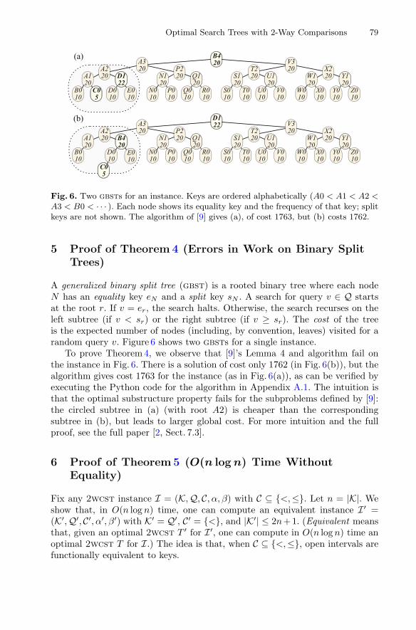
Fig. 6. Two gbsts for an instance. Keys are ordered alphabetically (A0 < A1 < A2 <A3 < B0 < · · · ). Each node shows its equality key and the frequency of that key; splitkeys are not shown. The algorithm of [9] gives (a), of cost 1763, but (b) costs 1762.

5 Proof of Theorem4 (Errors in Work on Binary SplitTrees)

A generalized binary split tree (gbst) is a rooted binary tree where each nodeN has an equality key eN and a split key sN . A search for query v ∈ Q startsat the root r. If v = er, the search halts. Otherwise, the search recurses on theleft subtree (if v < sr) or the right subtree (if v ≥ sr). The cost of the treeis the expected number of nodes (including, by convention, leaves) visited for arandom query v. Figure 6 shows two gbsts for a single instance.

To prove Theorem 4, we observe that [9]’s Lemma 4 and algorithm fail onthe instance in Fig. 6. There is a solution of cost only 1762 (in Fig. 6(b)), but thealgorithm gives cost 1763 for the instance (as in Fig. 6(a)), as can be verified byexecuting the Python code for the algorithm in Appendix A.1. The intuition isthat the optimal substructure property fails for the subproblems defined by [9]:the circled subtree in (a) (with root A2) is cheaper than the correspondingsubtree in (b), but leads to larger global cost. For more intuition and the fullproof, see the full paper [2, Sect. 7.3].

6 Proof of Theorem5 (O(n logn) Time WithoutEquality)

Fix any 2wcst instance I = (K,Q, C, α, β) with C ⊆ {<,≤}. Let n = |K|. Weshow that, in O(n log n) time, one can compute an equivalent instance I ′ =(K′,Q′, C′, α′, β′) with K′ = Q′, C′ = {<}, and |K′| ≤ 2n+1. (Equivalent meansthat, given an optimal 2wcst T ′ for I ′, one can compute in O(n log n) time anoptimal 2wcst T for I.) The idea is that, when C ⊆ {<,≤}, open intervals arefunctionally equivalent to keys.


Assume without loss of generality that C = {<,≤}. (Otherwise no correcttree exists unless K = Q, and we are done.) Assume without loss of generalitythat no two elements in Q are equivalent (in that they relate to all keys in Kin the same way; otherwise, remove all but one query from each equivalenceclass). Hence, at most one query lies between any two consecutive keys, and|Q| ≤ 2|K| + 1.

Let instance I ′ = (K′,Q, C′, α′, β′) be obtained by taking the key set K′ =Q to be the key set, but restricting comparisons to C′ = {<} (and adjustingthe probability distribution appropriately — take α′ ≡= 0, take βi to be theprobability associated with the ith query — the appropriate αj or βj).

Given any irreducible 2wcst T for I, one can construct a tree T ′ for I ′ ofthe same cost as follows. Replace each node 〈v ≤ k〉 with a node 〈v < q〉, whereq is the least query value larger than k (there must be one, since 〈v ≤ k〉 is in Tand T is irreducible). Likewise, replace each node 〈v < k〉 with a node 〈v < q〉,where q is the least query value greater than or equal to k (there must be one,since 〈v < k〉 is in T and T is irreducible). T ′ is correct because T is.

Conversely, given any irreducible 2wcst T ′ for I ′, one can construct anequivalent 2wcst T for I as follows. Replace each node N ′ = 〈v < q〉 as follows.If q ∈ K, replace N ′ by 〈v < k〉. Otherwise, replace N ′ by 〈v ≤ k〉, where key kis the largest key less than q. (There must be such a key k. Node 〈v < q〉 is inT ′ but T ′ is irreducible, so there is a query, and hence a key k, smaller than q.)Since T ′ correctly classifies each query in Q, so does T .

To finish, we note that the instance I ′ can be computed from I in O(n log n)time (by sorting the keys, under reasonable assumptions about Q), and thesecond mapping (from T ′ to T ) can be computed in O(n log n) time. Since I ′

has K′ = Q′ and C = {<}, it is known [10] to be equivalent to an instance ofalphabetic encoding, which can be solved in O(n log n) time [4,7].

A Appendix

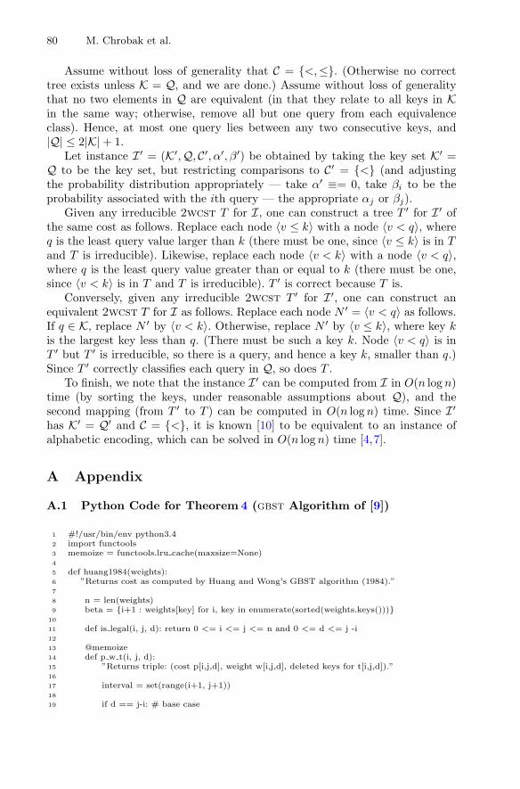
A.1 Python Code for Theorem4 (gbst Algorithm of [9])

1 #!/usr/bin/env python3.42 import functools3 memoize = functools.lru cache(maxsize=None)4

5 def huang1984(weights):6 ”Returns cost as computed by Huang and Wong's GBST algorithm (1984).”7

8 n = len(weights)9 beta = {i+1 : weights[key] for i, key in enumerate(sorted(weights.keys()))}

10

11 def is legal(i, j, d): return 0 <= i <= j <= n and 0 <= d <= j -i12

13 @memoize14 def p w t(i, j, d):15 ”Returns triple: (cost p[i,j,d], weight w[i,j,d], deleted keys for t[i,j,d]).”16

17 interval = set(range(i+1, j+1))18

19 if d == j-i: # base case


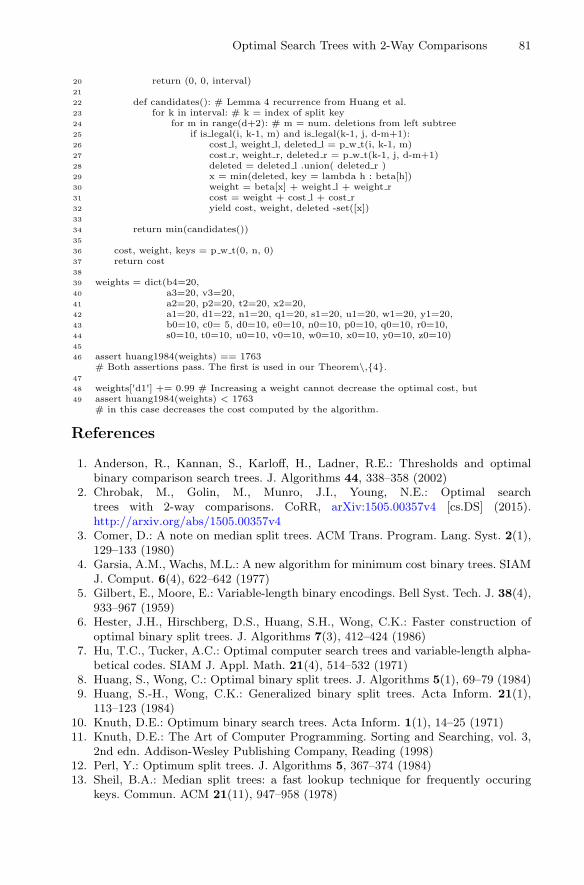
20 return (0, 0, interval)21

22 def candidates(): # Lemma 4 recurrence from Huang et al.23 for k in interval: # k = index of split key24 for m in range(d+2): # m = num. deletions from left subtree25 if is legal(i, k-1, m) and is legal(k-1, j, d-m+1):26 cost l, weight l, deleted l = p w t(i, k-1, m)27 cost r, weight r, deleted r = p w t(k-1, j, d-m+1)28 deleted = deleted l .union( deleted r )29 x = min(deleted, key = lambda h : beta[h])30 weight = beta[x] + weight l + weight r31 cost = weight + cost l + cost r32 yield cost, weight, deleted -set([x])33

34 return min(candidates())35

36 cost, weight, keys = p w t(0, n, 0)37 return cost38

39 weights = dict(b4=20,40 a3=20, v3=20,41 a2=20, p2=20, t2=20, x2=20,42 a1=20, d1=22, n1=20, q1=20, s1=20, u1=20, w1=20, y1=20,43 b0=10, c0= 5, d0=10, e0=10, n0=10, p0=10, q0=10, r0=10,44 s0=10, t0=10, u0=10, v0=10, w0=10, x0=10, y0=10, z0=10)45

46 assert huang1984(weights) == 1763# Both assertions pass. The first is used in our Theorem\,{4}.

47

48 weights['d1'] += 0.99 # Increasing a weight cannot decrease the optimal cost, but49 assert huang1984(weights) < 1763

# in this case decreases the cost computed by the algorithm.

References

1. Anderson, R., Kannan, S., Karloff, H., Ladner, R.E.: Thresholds and optimalbinary comparison search trees. J. Algorithms 44, 338–358 (2002)

2. Chrobak, M., Golin, M., Munro, J.I., Young, N.E.: Optimal searchtrees with 2-way comparisons. CoRR, arXiv:1505.00357v4 [cs.DS] (2015).http://arxiv.org/abs/1505.00357v4

3. Comer, D.: A note on median split trees. ACM Trans. Program. Lang. Syst. 2(1),129–133 (1980)

4. Garsia, A.M., Wachs, M.L.: A new algorithm for minimum cost binary trees. SIAMJ. Comput. 6(4), 622–642 (1977)

5. Gilbert, E., Moore, E.: Variable-length binary encodings. Bell Syst. Tech. J. 38(4),933–967 (1959)

6. Hester, J.H., Hirschberg, D.S., Huang, S.H., Wong, C.K.: Faster construction ofoptimal binary split trees. J. Algorithms 7(3), 412–424 (1986)

7. Hu, T.C., Tucker, A.C.: Optimal computer search trees and variable-length alpha-betical codes. SIAM J. Appl. Math. 21(4), 514–532 (1971)

8. Huang, S., Wong, C.: Optimal binary split trees. J. Algorithms 5(1), 69–79 (1984)9. Huang, S.-H., Wong, C.K.: Generalized binary split trees. Acta Inform. 21(1),

113–123 (1984)10. Knuth, D.E.: Optimum binary search trees. Acta Inform. 1(1), 14–25 (1971)11. Knuth, D.E.: The Art of Computer Programming. Sorting and Searching, vol. 3,

2nd edn. Addison-Wesley Publishing Company, Reading (1998)12. Perl, Y.: Optimum split trees. J. Algorithms 5, 367–374 (1984)13. Sheil, B.A.: Median split trees: a fast lookup technique for frequently occuring

keys. Commun. ACM 21(11), 947–958 (1978)

http://arxiv.org/abs/1505.0035

http://arxiv.org/abs/1505.0035


14. Spuler, D.: Optimal search trees using two-way key comparisons. Acta Inform. 740,729–740 (1994)

15. Spuler, D.A.: Optimal search trees using two-way key comparisons. Ph.D. thesis,James Cook University (1994)

16. Yeung, R.: Alphabetic codes revisited. IEEE Trans. Inf. Theory 37(3), 564–572(1991)

optimal search trees with 2-way comparisonsneal/chrobak15optimal.pdf · optimal search trees with...

Documents