optimal realizations of floating-pointimplemented digital

Optimal Realizations of Floating-Point Implemented DigitalControllers with Finite Word Length Considerations

Jun Wu �, Sheng Chen � �, James F. Whidborne � and Jian Chu �

� National Key Laboratory of Industrial Control TechnologyInstitute of Advanced Process ControlZhejiang University, Hangzhou, 310027, P. R. China

� School of Electronics and Computer ScienceUniversity of Southampton, HighfieldSouthampton SO17 1BJ, U.K.

� Department of Aerospace SciencesSchool of Engineering, Cranfield UniversityBedfordshire MK43 0AL, U.K.

Abstract

The closed-loop stability issue of finite word length (FWL) realizations is investigated for digital con-

trollers implemented in floating-point arithmetic. Unlike the existing methods which only address the

effect of the mantissa bits in floating-point implementation to the sensitivity of closed-loop stability,

the sensitivity of closed-loop stability is analyzed with respect to both the mantissa and exponent bits

of floating-point implementation. A computationally tractable FWL closed-loop stability measure is

then defined, and the method of computing the value of this measure is given. The optimal controller

realization problem is posed as searching for a floating-point realization that maximizes the proposed

FWL closed-loop stability measure, and a numerical optimization technique is adopted to solve for the

resulting optimization problem. Simulation results show that the proposed design procedure yields com-

putationally efficient controller realizations with enhanced FWL closed-loop stability performance.

Index Terms — digital controller, finite word length, floating-point, closed-loop stability, optimization.

1 Introduction

The classical digital controller design methodology often assumes that the controller is implemented

exactly, even though in reality a control law can only be realized in finite precision. It may seem that

the uncertainty resulting from finite-precision implementation of the digital controller is so small, com-

0Contact author. Tel/Fax: +44 (0)23 8059 6660/4508; Email: [email protected]

1

pared to the uncertainty within the plant, such that this controller “uncertainty” can simply be ignored.

Increasingly, however, researchers have realized that this is not necessarily the case. Due to the finite

word length (FWL) effect, a casual controller implementation may degrade the designed closed-loop

performance or even destabilize the designed stable closed-loop system, if the controller implementa-

tion structure is not carefully chosen. The effects of finite-precision implementation have become more

critical with the growing popularity of robust controller design methods which focus only on dealing

with large plant uncertainty (Keel & Bhattacharryya, 1997; Istepanian & Whidborne, 2001). Generally

speaking, there are two types of FWL errors in the digital controller. The first one is perturbation of

controller parameters implemented with FWL and the second one is the rounding errors that occur in

arithmetic operations of signals. Typically, effects of these two types of errors are investigated separately

for the reason of mathematical tractability. The first type of FWL errors directly concerns with the critical

issue of closed-loop stability, and many studies have investigated some closed-loop stability robustness

measures, especially for fixed-point implementation (Fialho & Georgiou, 1994, 2001; Madievski et al.,

1995; Li, 1998; Chen et al., 1999; Whidborne et al., 2000, 2001; Wu et al., 2001a, 2001b). The second

type of FWL errors can also lead to instability through bounded limit cycles or floating point unbounded

responses and how to erase its effect on stability is the focus of the work of many researchers in control

or digital filter system designs (Liu & Kaneko, 1969; Kaneko, 1973; Miller et al., 1988, 1989; Bauer &

Wang, 1993; Bauer, 1995). Even when it does not arouse unstable behaviour, the second type of FWL

errors can still degrade the system performance and the effect of this is usually measured and studied with

the so-called roundoff noise gain (Moroney et al., 1980; Williamson & Kadiman, 1989; Li & Gevers,

1990; Li et al., 2002; Liu et al., 1992).

Most works for FWL controller design adopt an indirect strategy, which relies on the following prop-

erty. A control law can be implemented with different realizations, and these different realizations are

all equivalent if they are implemented in infinite precision. However, different controller realizations

possess different degrees of robustness to FWL errors. The control law is assumed to be given by some

controller design methods, which may not take into account FWL considerations, and the FWL design

is to select optimal realizations for the given control law by optimizing some FWL criteria. An alterna-

tive but better approach is to explicitly incorporate the FWL issues into controller design process. For

example, in the work of Liu et al. (1992), an FWL-LQG performance index was used to describe the

LQG performance under FWL environment, and a fixed-order controller realization design method was

presented to minimize this FWL-LQG cost function. This direct strategy should be a preferred approach,

since it does not make specific assumptions on the controller. However, how to extend the idea of Liu et

2

al. (1992) to various controller design methods is still an open problem. But this difficulty does not exist

in the indirect strategy where controller synthesis and controller realization are two separate steps. Var-

ious existing controller design methods can be used to attain a transfer function or an initial realization

of the controller, which can then be optimized to satisfy FWL implementation requirements.

In real-time applications where computational efficiency is critical, a digital controller implemented

with fixed-point arithmetic has some advantages over floating-point format. However, the detrimental

FWL effects are markedly increased in fixed-point implementation due to a reduced precision. It is

therefore not surprising that previous works have focused on finding optimal controller realizations using

fixed-point arithmetic by optimizing some FWL measures (Chen et al., 1999; Fialho & Georgiou, 1994,

2001; Gevers & Li, 1993; Li & Gevers, 1990; Li 1998; Li et al., 2002; Liu et al., 1992; Madievski

et al., 1995; Whidborne et al., 2000, 2001; Wu et al., 2001a, 2001b). In all the previous works using

fixed-point arithmetic, various measures, which can be shown to link to the bits required in implementing

the fractional part of fixed-point representation, are optimized to produce optimal realizations. However,

the dynamic range of fixed-point representation is determined by its integer part. Overflow occurs when

there are not enough bits for the integer part. Optimizing these measures, while minimizing the bits

required for the fractional part, may actually increase the bits required for the integer part. Arguably, a

better approach would be to consider some measure which has a direct link to the total bit length required.

With decreasing in price and increasing in availability, the use of floating-point processors in con-

troller implementations has increased dramatically. Floating-point representation has quite different

characteristics from fixed-point representation. The dynamic range of floating-point representation is

determined by its exponent part. Overflow or underflow occurs when the bits for the exponent part are

not sufficient. The effects of finite-precision floating-point implementation have been well studied in

digital filter designs (Rao, 1996; Kalliojarvi & Astola, 1996; Ralev & Bauer, 1999). However, there has

been relatively little work studying explicitly floating point digital controller implementations. Some

exceptions include Rink & Chong (1979), Molchanov & Bauer (1995), Whidborne & Gu (2002). In the

work by Istepanian et al. (2000), a block-floating-point arithmetic was used, in which control coeffi-

cients were forced to have a common exponent and the problem was converted into a fixed-point one.

The work by Whidborne & Gu (2002) represents a case of true floating-point implementation. In this

work, a weighted closed-loop eigenvalue sensitivity index was defined for floating-point digital controller

realizations. This index, however, only considers the mantissa part of floating-point arithmetic, under an

assumption that the exponent bits are unlimited.

3

This paper adopts an indirect approach to consider the FWL parameter errors of floating-point imple-

mented controllers. The generic contribution of this paper is to derive a new FWL closed-loop stability

measure that explicitly considers both the mantissa and exponent parts of floating-point arithmetic. The

remainder of this paper is organized as follows. Section 2 briefly summarizes the floating-point rep-

resentation and highlights the multiplicative nature of perturbations resulting from FWL floating-point

arithmetic. Section 3 analyses the FWL effect of floating-point arithmetic on closed-loop stability and

addresses how to measure such an effect on floating-point implemented digital controllers. Section 4 de-

fines a computationally tractable FWL closed-loop stability measure for floating-point controller realiza-

tions and provides the method of computing its value. In section 5, the optimal floating-point controller

realization problem is formulated, and a numerical optimization technique is adopted to solve for the

resulting optimization problem. Two examples are given in section 6 to demonstrate the effectiveness of

the proposed design method. Section 7 presents a brief discussion on the direct approach of Liu et al.

(1992) and points out that the studies on optimizing FWL realizations for a fixed control law, such as

this work, are helpful to explore the possible way of extending the idea of Liu et al. (1992). The paper

concludes at section 8.

2 Floating-Point Representation

Let the floor function �� denote the largest integer less than or equal to real number �. It is well known

that any real number � � � can be represented uniquely by

� � �� (1)

where � � �� is for the sign of �, � � �� is the mantissa of �, � � �� is the

exponent of � with denoting the set of integers. When � is stored in a digital computer of finite � bits

in a floating-point format, the bits consist of three parts: one bit for �, �� bits for � and �� bits for �.

Obviously,

� � � � �� (2)

As the finite �� bits can only support a limited exponent range, we define � and � to represent the lower

and upper limits of the exponent range, respectively, and denote the exponent range that is supported by

�� bits as

�� (3)

In fact, the exponent range �� depends on not only �� but also the set of real numbers which is to be

represented. As an example, consider the set of three numbers �� . At

4

least 2 bits are required to describe their exponents, with �� representing ��, �� for �, �� representing

� and �� for 2. Thus, � � ��, � � � and �� are determined by the three numbers

represented in this example of exponent bits �� . Obviously

�� (4)

Overflow and underflow can occur in float-point arithmetic of FWL. Overflow occurs when a floating-

point scheme with �� is used to represent a real number whose exponent is greater than �, while

underflow occurs when a floating-point scheme with �� is used to represent a real number whose

exponent is smaller than �. It should be emphasized that in many practical problems, the problem ob-

jective function is highly sensitive to small parameter perturbation and, therefore, small numbers should

not simply be “underflowed” to zero. For a demonstration, we refer to the so-called fragility issue (Keel

& Bhattacharryya, 1997). In floating-point arithmetic with FWL, underflow should generally be treated

as seriously as overflow, and avoided if possible.

Since �� and �� are finite, the set of numbers that is represented by a particular floating-point scheme

is not dense on the real line. Thus the set of possible floating-point numbers is given by

��

��

��

��

��

��

� � �� (5)

When no underflow or overflow occurs, that is, the exponent of � is within �� , the floating-point

quantization operator � �� can be defined as

��

��

�� for � ��

�� for � � �(6)

In the above definition, magnitude rounding is used as the mantissa quantization format. Define the

quantization error � as

�� (7)

Then

� ��

��

�� (8)

From the definition of the exponent �, we have

�� (9)

5

Combining (8) and (9) leads to

� �� (10)

Thus, when � is implemented in floating-point format of �� mantissa bits, assuming no underflow or

overflow, it can be seen from (7) and (10) that � is perturbed to

�� Æ�� Æ� �� (11)

Clearly, the perturbation resulting from finite-precision floating-point arithmetic is multiplicative, unlike

the perturbation resulting from finite-precision fixed-point arithmetic, which is additive.

3 Problem Statement

Consider the discrete-time closed-loop control system, consisting of a linear time invariant plant ��

and a digital controller ��. The plant model �� is assumed to be strictly proper with a state-space de-

scription �� , where�� ,�� and�� . Let ��

be a state-space description of the controller ��, with �� , �� , �� and

�� . A linear system with a given transfer function matrix has an infinite number of state-

space descriptions. In fact, if ��

��

��

�� is a state-space description of ��, all the state-space

descriptions of �� form a realization set

��

��

��

(12)

where the transformation matrix � � �� is an arbitrary non-singular matrix. Denote

� � ��

��

��

�� (13)

The stability of the closed-loop control system depends on the eigenvalues of the closed-loop transition

matrix

��

��

��

��

��

� �

��

��

� ��

��

��

� ��

�

�� (14)

where � denotes the zero matrix of appropriate dimension and �� the � � � identity matrix. All the

different realizations � in �� have exactly the same set of closed-loop poles if they are implemented

with infinite precision. Since the closed-loop system has been designed to be stable, all the eigenvalues

��, � � �� , are within the unit disk. Define

��

�� (15)

6

and

��

�� (16)

The controller � is implemented with a floating-point processor of �� exponent bits, �� mantissa bits

and one sign bit.

Firstly, in order to avoid underflow and/or overflow, both the exponent of �� and the exponent

of �� should be within �� supported by the �� exponent bits. We define an exponent measure for

the floating-point controller realization � as

��

��

��

�� (17)

The rationale of this exponent measure becomes clear in the following (obvious) proposition.

Proposition 1 � can be represented in the floating-point format of �� exponent bits without underflow

or overflow, if ��

��

�� .

Let �� be the smallest exponent bit length that, when used to implement �, can avoid underflow

and overflow. It can be computed as

�� (18)

The measure �� provides an estimate of �� as

��

�� (19)

It is clear that ��

� .

Secondly, when there is no underflow or overflow, according to (11), � is perturbed to � �� Æ

due to the effect of finite �� where

� Æ�� Æ �� (20)

represents the Hadamard product of � and � �Æ ��. Each element of is bounded by ��,

that is,

�� (21)

With the perturbation , �� is moved to ��Æ��. If an eigenvalue of��Æ�

is outside the open unit disk, the closed-loop system, designed to be stable, becomes unstable with the

finite-precision floating-point implemented �.

7

It is therefore critical to know when the FWL error will cause closed-loop instability. This means

that we would like to know the largest open “hypercube” in the perturbation space, within which the

closed-loop system remains stable. Based on this consideration, a mantissa measure for the floating-

point realization � can be defined as

�� Æ� is unstable� � (22)

From the above definition, the following proposition is obvious.

Proposition 2 �� Æ� is stable if �� .

Let �� be the mantissa bit length such that ��

� ,�� Æ� is stable for the floating-

point implemented � with �� mantissa bits and�� Æ� is unstable for the floating-point imple-

mented� with �� mantissa bits. Except through simulation, ��

� is generally unknown. It should

be pointed out that due to the complex nonlinear relationship between �� and closed-loop stability, there

may exist some odd cases of smaller mantissa bit length �� which regain closed-loop

stability. For example, consider the stable closed-loop system containing the plant

��

��

and the controller �� . When �� , the closed-loop system with the FWL implemented

� is stable, but it becomes unstable with �� where the implemented value of � is ��. However,

the closed-loop regains stability with �� where the implemented value of � is ��. The system

becomes unstable again for �� where the implemented value of � is ��. Figure 1 shows the root

locus plot of this 3-order system which gives the closed-loop pole positions for all values of � . From

Figure 1, it can be seen that the system is unstable when the implemented value of � is greater than

�� or less than ��. For this system, �� is 4 rather than 2. The mantissa measure �� provides

an estimate of �� as

��

�� (23)

It can be seen that ��

� .

Define the minimum total bit length required in floating point implementation as

��

� � �� (24)

Clearly, a floating-point implemented � with a bit length � � �� can guarantee no underflow, no

overflow and closed-loop stability. Combining the measures �� and �� results in the following

8

true FWL closed-loop stability measure for the floating-point realization �

�� (25)

An estimate of �� is given by �� as

��

�� (26)

It is clear that �� . The following proposition summarizes the usefulness of �� as a

measure for the FWL characteristics of�.

Proposition 3 A floating-point implemented� with a bit length � can guarantee no underflow, no over-

flow and closed-loop stability, if

��

�� (27)

Since the closed-loop stability measure �� is a function of the controller realization � and ��

decreases with the increase of ��, an optimal realization can in theory be found by maximizing

��, leading to the following optimal controller realization problem

��

�� (28)

However, the difficulty with this approach is that computing the value of �� is an unsolved open

problem. Thus, the true FWL closed-loop stability measure �� and the optimal realization problem

(28) have limited practical significance. In the next section, we will seek an alternative measure that not

only can quantify FWL characteristics of � but also is computationally tractable.

4 A Tractable FWL Closed-Loop Stability Measure

When the FWL error is small, from a first-order approximation, ��

� �� Æ��

��

��

�Æ ��

��

Æ �� (29)

For the derivative matrix ��

��Æ��

�, define

��

��

��

�� Æ ��

�� (30)

Then

� �� Æ��

��

��

��

� (31)

9

This leads to the following mantissa measure for the floating-point realization �

��

��

��

��

��

� (32)

For those FWL errors that make (31) hold, if �� , then � �� Æ�� which

means that the closed-loop remains stable under the FWL error . In other words, the closed-loop can

tolerate those FWL perturbations whose norms �� are less than ��. The larger �� is,

the larger FWL errors the closed-loop system can tolerate. Similar to (23), from the mantissa measure

��, an estimate of �� is given as

��

�� (33)

The assumption of small is usually valid in floating-point implementation. Generally speaking,

there is no rigorous relationship between �� and ��, but �� is connected with a lower bound

of �� in some manners: there are “stable perturbation hypercubes” larger than � � ��

�� while there is no “stable perturbation hypercube” larger than � � �� (Wu et

al., 2000, 2001a). Hence, in most cases, it is reasonable to take that �� and ��

�� .

More importantly, unlike the measure ��, the value of �� can be computed explicitly. It is easy

to see that

��

�

��

��

��Æ� � (34)

Let � be a right eigenvector of�� corresponding to the eigenvalue �. Define

�� (35)

and

��

� (36)

where the superscript � denotes the conjugate transpose operator and �� is called the reciprocal left

eigenvector related to �. The following lemma is due to Li (1998).

Lemma 1 Let�� given in (14) be diagonalizable. Then

� ��

��

��

��

�� (37)

where the superscript � denotes the conjugate operation and � the transpose operator.

10

Comments: The necessary and sufficient condition for �� being diagonalizable is that it has � � �

linearly independent eigenvectors. This includes two cases. Firstly,�� has �� distinct eigenvalues.

In this case, we can differentiate eigenvalues simply by their values. Secondly, the eigenvalues of��

are not all distinct but there are �� linearly independent eigenvectors. In this case, we can differentiate

eigenvalues by their corresponding eigenvectors.

The following proposition shows that, given a�, the value of �� can easily be calculated.

Proposition 4 Let�� be diagonalizable. Then

��

� ��

��

��

�

�Æ�

��

� (38)

Proof: Noting � �� leads to

��

��

�

��

��

� � ��

��

�

��

��

��

� ��

��

�

� ��Re

� ��

� ��

�� (39)

Combining (32), (34), (39) and Lemma 1 results in this proposition.

Replacing �� with �� in (25) leads to a computationally tractable FWL closed-loop stability

measure

�� (40)

From the above measure, an estimate of �� is given as

��

�� (41)

Note that the computationally tractable mantissa measure (32) is related to the eigenvalue module

sensitivities with respect to (w.r.t.) the controller perturbation. This is similar to the case of controller

realizations implemented in fixed-point arithmetic, where an existing FWL precision measure is defined

as (Wu et al., 2001a)

��

��

��

��

� (42)

The idea underpinning �� in (32), namely the sensitivity w.r.t. controller perturbation, is the same

as the sensitivity w.r.t. controller parameters that underpins �� in (42). In fact, it is well-known that

with an FWL fixed-point implementation, � is perturbed to �� and

� ��

��

��

�Æ ��

��

Æ �� (43)

11

Obviously, in the fixed-point case, we have

��

�

��

��

�� (44)

and the fixed-point FWL measure �� can be written as

��

��

��

��

� (45)

On the other hand, from (32) and (34), it can be seen that

��

�� Æ��

� (46)

which is clearly linked to the eigenvalue module sensitivities w.r.t. the controller parameters. The

Hadamard product in (46) merely reflects the multiplicative characteristic of floating-point perturbations.

It is also useful to compare the proposed measure with the previous results for floating-point format,

especially the most recent one given by Whidborne & Gu (2002). For a complex-valued matrix � �

�� , define the Frobenius norm

��

��

��

��

��

��

� (47)

Under an assumption that the exponent bits are unlimited, the computationally tractable weighted closed-

loop eigenvalue sensitivity index addressed in (Whidborne & Gu, 2002) is given by

��

��

�� (48)

where �� are non-negative weighting scalars and �� are single-eigenvalue sensitivities defined by

��

��

��

�� (49)

The thinking behind the above definition is as follows. From a first-order approximation, it can easily be

shown that

� �� Æ��

��

�� (50)

Therefore, for those multiplicative perturbations bounded by �� , a small �� will limit the

resulting change of the corresponding eigenvalue within a small range.

The first obvious observation is that �� considers both the mantissa and exponent of floating-

point arithmetic and is therefore able to handle all the aspects of underflow, overflow and closed-loop

12

stability, while �� only considers the mantissa part of floating-point arithmetic and is thus “incom-

plete”. Secondly, it can be seen that �� deals with the sensitivity of � while �� (��) consid-

ers the the sensitivity of � ��. It is well-known that the stability of a discrete-time linear time-invariant

system depends only on the moduli of its eigenvalues. As �� includes the unnecessary eigenvalue

arguments in consideration, it is generally conservative in comparison with ��. Thirdly, �� uses�� Æ��

while �� uses ��

��

in checking the change of an eigenvalue. It is easy to see

that

� �� Æ��

�� Æ�

��

��

��

�� (51)

Obviously,�� Æ�

��

gives a more accurate limit than ��

��

does on the change of the

corresponding eigenvalue module due to the multiplicative perturbations. This again implies that ��

is less conservative than �� in estimating the robustness of closed-loop stability with respect to con-

troller perturbations. The fourth observation is that �� provides an estimate of ��, �� in (41),

while �� cannot provide information on bit length to the designer. One reason is that the measure

�� consists of two components, with �� addressing the stability margin and eigenvalue sensi-

tivity linked to the mantissa bits, and �� considering the exponent bits, while �� only focuses

on the eigenvalue sensitivity partially linked to the mantissa part. The other reason is that, over all the

closed-loop eigenvalues, �� considers the “worst” one while �� considers a “weighted average”.

Finally, it is worth emphasizing that the generic idea of considering both the exponent, which defines

the dynamic range, and mantissa, which defines the accuracy or precision, of the floating-point arithmetic

is a sensible one and should be extended to other situations where different representation schemes, such

as fixed-point format, are used.

5 Optimization Procedure

As different realizations � have different values of the FWL closed-loop stability measure ��, it is

of practical importance to find an “optimal” realization �� that maximizes ��. The controller im-

plemented with this optimal realization �� needs a minimum bit length and has a maximum tolerance

to the FWL error. This optimal controller realization problem is formally defined as

��

�� (52)

13

Assume that a controller has been designed using some standard controller design method. This con-

troller, denoted as

��

��

� ��

��

�

�� (53)

is used as the initial controller realization in the above optimal controller realization problem. Let�� be a

right eigenvector of�� corresponding to the eigenvalue �, and �� be the reciprocal left eigenvector

related to ��. The definition of �� in (12) means that

��

��

� ��

��

��

� �

�(54)

where �� . It can then be shown that

��

��

� ��

��

��

� �

�(55)

which implies that

� �

��

� ��

��

��

� ��

�� (56)

Hence

��

��

��

� �

��

� ��

��

� ��

��

��

��

� ��

��

��

� ��

� �

��

� ��

�(57)

with � ��

��

��

�� . Define the following cost function:

��

��

��

� ��

� �

��

� ��

��Æ��

��

� ��

��

��

�� (58)

In the above definition of the cost function ��,

��

��

is simply �� which estimates the cost of exponent bits, while

��

��

� ��

� �

��

� ��

��Æ��

��

� ��

is the inverse of �� which estimates the cost of mantissa bits. Hence �� can be used to measure

the cost of total bits.

With the introduction of this cost function, the optimal controller realization problem (52) can then

be posed as the following optimization problem:

��

��

�� (59)

14

As the optimization problem (59) is highly nonlinear, global optimization algorithms, such as the genetic

algorithm (Man et al., 1998) and adaptive simulated annealing (Chen & Luk, 1999), can be adopted to

provide a (sub)optimal similarity transformation ��. Global optimization methods are however com-

putationally demanding. Local optimization algorithms, such as Rosenbrock and Simplex algorithms

(Beveridge & Schechter, 1970), are computationally simpler but run more risks of only attaining a lo-

cal solution. Our experience with the optimization problem (59) suggests that, unlike optimizing the

mantissa measure �� alone, the exponent measure �� in the criterion �� helps to bound the

solution set and the cost function �� appears to behave better. It is also helpful to use some good

initial controller realization, such as the open-loop balanced realization (Laub et al., 1987), as the initial

guess for the optimization routine. With ��, the optimal realization �� can readily be computed.

6 Numerical Examples

Two examples are used to illustrate the proposed design procedure for obtaining optimal FWL floating-

point controller realizations and to compare it with the method given in (Whidborne & Gu, 2002). In the

simulation, the bit length for implementing the state variables was sufficiently long such that the second

type of FWL errors can be neglected.

Example 1. This example, taken from (Gevers & Li, 1993), has been studied by Whidborne & Gu

(2002). The discrete-time plant is given by

��

��

��

!""# �

��

��

The initial realization of the digital controller is given by

��

��

��

��

!"""# �

��

��

� � � �

Based on the proposed FWL closed-loop stability measure, the optimization problem (59) was formed

and solved for using the MATLAB routine fminsearch.m, which is a local optimization search algorithm,

15

to obtain an optimal transformation matrix

��

��

��

!"""#

and the corresponding optimal realization of the digital controller �� given by

��

��

��

��

!"""# �

��

��

��

An “optimal” controller realization problem was given in (Whidborne & Gu, 2002) based on the

weighted closed-loop eigenvalue sensitivity index (48). We will use the index “s”, rather then “opt”, to

denote the solution of this “optimal” controller realization problem. For this example, the transformation

matrix solution obtained using the MATLAB routine fminsearch.m given in (Whidborne & Gu, 2002) is

��

��

!""#

with the corresponding controller realization �� given by

��

��

��

��

!"""# �

��

��

� � � �

It is obvious that the true minimum exponent bit length �� for a realization � can directly be

obtained by examining the elements of �. The true minimum mantissa bit length �� however can

only be obtained through simulation. That is, starting from a very large ��, reduce �� by one bit and

check the closed-loop stability. The process is repeated until there appears closed-loop instability at

�� . Then �� . Table 1 summarizes the various measures, the corresponding

estimated minimum bit lengths and the true minimum bit lengths for the three controller realizations��,

�� and ��, respectively. It can be seen that the floating-point implementation of �� needs at least 26

bits (20 mantissa bits and 5 exponent bits) while the implementation of �� needs at least 13 bits (8

16

mantissa bits and 4 exponent bits). The reduction in the bit length required is 13 (12-bit reduction for the

mantissa part and 1-bit reduction for the exponent part). Comparing �� with ��, it can be seen that

�� needs one bit less in the exponent part and one bit less in the mantissa part.

Notice that any realization � � �� implemented in infinite precision will achieve the exact per-

formance of the infinite-precision implemented ��, which is the designed controller performance. For

this reason, the infinite-precision implemented �� is referred to as the ideal controller realization �� .

Figure 2 compares the unit impulse response of the plant output �� for the ideal controller �� with

those of the 8-mantissa-bit plus 5-exponent-bit implemented �� and 8-mantissa-bit plus 4-exponent-bit

implemented ��. The 8-mantissa-bit implemented �� quickly becomes unstable and is not shown

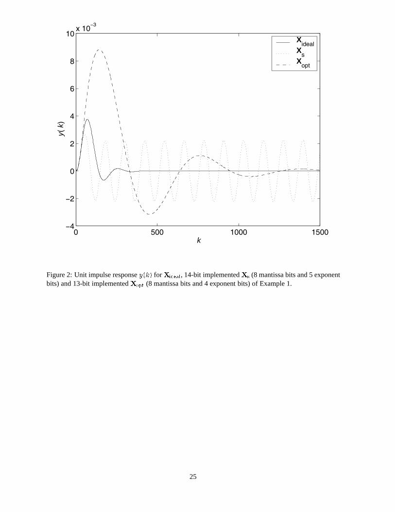
here. From Figure 2, it can be seen that the closed-loop system with the 13-bit implemented �� is

stable while the system with the 14-bit implemented �� is unstable. Figure 3 compares the unit impulse

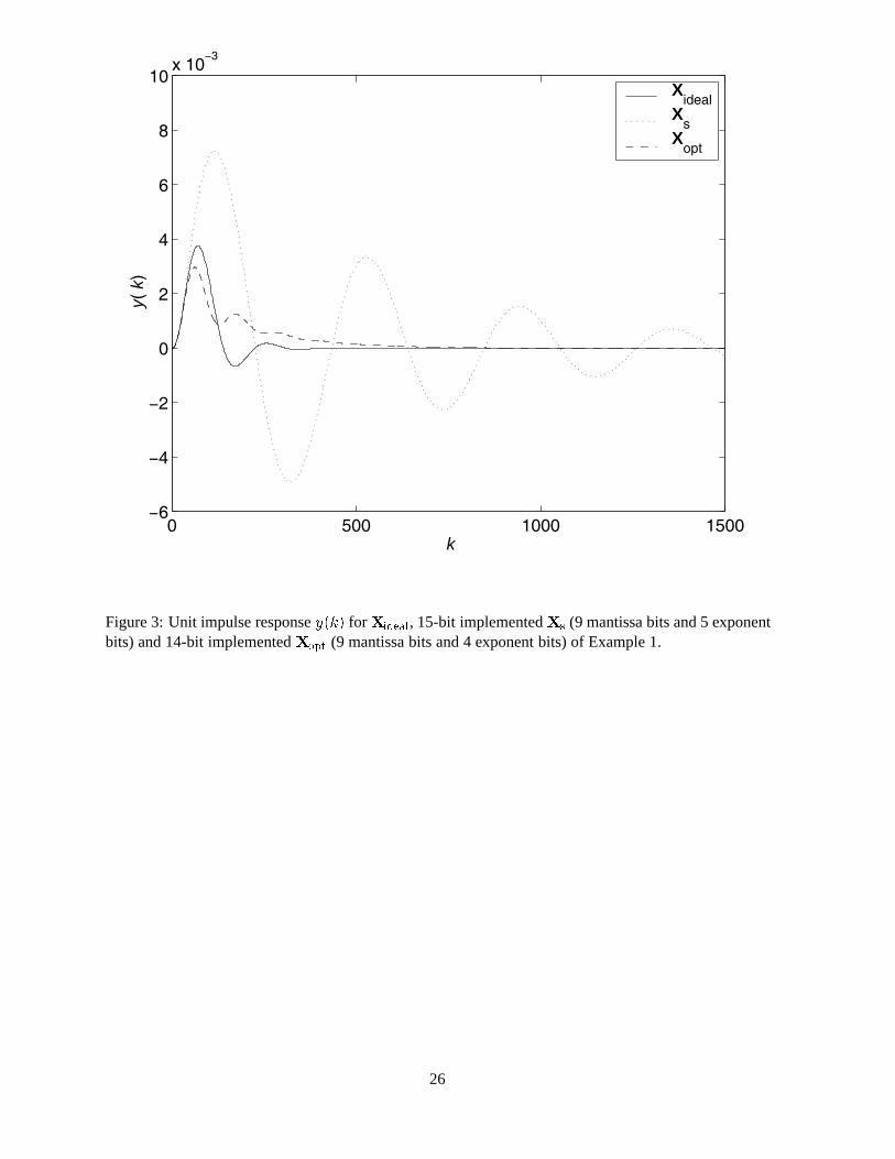
response of �� for �� with those of the 9-mantissa-bit plus 5-exponent-bit implemented �� and

the 9-mantissa-bit plus 4-exponent-bit implemented ��. Again the 9-mantissa-bit implemented �� is

unstable and is not shown. It can be seen that the response with the 14-bit implemented �� is clearly

closer to the ideal performance than that of the 15-bit implemented ��.

Example 2. This example is taken from a continuous-time �� robust control example studied in (Keel

& Bhattacharryya, 1997; Whidborne et al., 2001). The continuous-time plant model and �� controller

are sampled with a sampling period of 4 ms to obtain the discrete-time plant

��

��

� �

��

��

and the initial realization of the digital controller

��

� ��

� � ��

!# �

��

��

� � ��

The MATLAB routine fminsearch.m was used to solve for the optimization problem based on the FWL

closed-loop stability measure presented in this paper to obtain an optimal transformation matrix

��

��

��

!"#

17

and the corresponding optimal realization of the digital controller �� with

��

��

!"# �

��

��

��

Based on the method of the weighted closed-loop eigenvalue sensitivity index (Whidborne & Gu, 2002),

the MATLAB routine fminsearch.m found a transformation matrix solution

��

� ��

!#

with the corresponding controller realization �� given by

��

��

��

!"# �

��

��

� � ��

Table 2 summarizes the various measures, the corresponding estimated minimum bit lengths and the

true minimum bit lengths for ��, �� and ��. Obviously, the implementation of �� needs at least 30

bits (25 mantissa bits and 4 exponent bits) while the implementation of �� requires at least 12 bits (7

mantissa bits and 4 exponent bits). It can be seen that the optimization results in a reduction of 18 bits for

the mantissa part. It is interesting to note that the realization ��, while reducing 16 bits in the required

�� , actually increases the required ��

� by one bit, compared with��. This is not surprising, since the

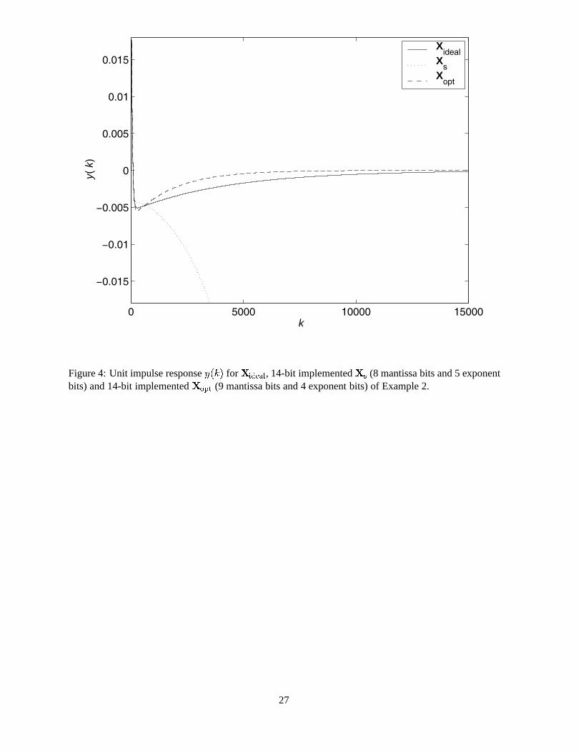
measure �� completely neglects the exponent part. Figure 4 compares the unit impulse response of

the plant output �� for the ideal controller �� with those of the 14-bit implemented �� (8 mantissa

bits and 5 exponent bits) and the 14-bit implemented �� (9 mantissa bits and 4 exponent bits). It can

be seen that the closed-loop system with the 14-bit implemented�� is stable while the system with the

14-bit implemented �� is unstable. Figure 5 compares the unit impulse response of �� for�� with

those of the 15-bit implemented �� (9 mantissa bits and 5 exponent bits) and the 15-bit implemented

�� (10 mantissa bits and 4 exponent bits). The performance of the 15-bit implemented�� is clearly

closer to the ideal performance than that of the 15-bit implemented ��.

18

7 Brief Discussion on the Direct Approach

A limitation of the indirect strategy, one may argue, is that it relies on a fixed control law or transfer

function. The direct approach removes this assumption and appears to be a better approach in dealing

with the FWL issues. Apart from the excellent work by Liu et al. (1992), we are only aware of another

case of successfully adopting a direct strategy (Yang et al., 2000), where the standard �� control design

was extended to include FWL controller parameter perturbations, and a Riccati inequality approach

was developed to directly obtains optimal controller realizations satisfying both the �� robustness and

FWL closed-loop stability requirements. Except for �� and LQG, it seems to be very difficult to

extend various controller design methods to this direct strategy. The indirect approach, however, is

very flexible. Controller synthesis is generally a highly complicated task, involving many trade-offs for

various conflicting requirements. Even when a direct method can be found, the indirect approach is still

useful, as it can be used to further optimize a controller realization obtained with the direct approach.

To see where the difficulties are for the direct approach, let us discuss how to extend the work of Liu

et al. (1992) to the generic setting. First define the controller realization set

�� is a controller realization stabilizing �� (60)

Assume that a performance index can be formulated to reflect the needs of all the performance require-

ments, including FWL implementation considerations. Extending the idea of Liu et al. (1992) to this

generic setting, the optimization problem1 for FWL controller realization design can be defined as

��

��

��

�� (61)

The cost function

��

��

�(62)

depends on �� and �, where � �� represents the average value, �� is the output of ��, �� is the

output of ��, � and � are given matrices. It is easy to see that the problem (61) can be broken into

two parts and solved for with the two coupling optimization problems:

!��

��

��

�� (63)

� � ��

!�� (64)

1There appeared �� (the fractional wordlength storing state variable) in the original problem of Liu et al. (1992). We omit�� here as it has no relevance to our discussion.

19

Providing that the optimization problem (63) can be solved exactly, for example, some close-form so-

lution of the problem (63) can be obtained, the optimization problem (64) can be tackled and hopefully

solved successfully. Apart from few performance cost functions, how to solve the generic optimization

problem (61) is still an open problem. It is also clear that the first part (63) of the optimization problem

(61) has the same form as our optimization problem (59). Thus, the studies on optimal realizations for a

fixed control law, like the one in this paper, may provide useful insights to help solving the more generic

optimal realization problem (61).

8 Conclusions

The closed-loop stability issue of finite-precision realizations has been investigated for digital controller

implemented in floating-point arithmetic. A new computationally tractable FWL closed-loop stability

measure has been derived for floating-point controller realizations. Unlike the existing methods, which

only consider the mantissa part of floating-point scheme, the proposed measure takes into account both

the exponent and mantissa parts of floating-point format. It has been shown that this new measure

yields a more accurate estimate for the FWL closed-loop stability. Based on this FWL closed-loop

stability measure, the optimal controller realization problem has been formulated, which can then be

solved for using numerical optimization algorithms. Two numerical examples have demonstrated that

the proposed design procedure yields computationally efficient controller realizations suitable for FWL

float-point implementation in real-time applications. The idea of considering both the dynamic range and

precision of FWL floating-point arithmetic is generic and can be used to deal with the similar problems

in FWL fixed-point arithmetic and FWL block-floating-point arithmetic. In fact, the implementation of

a digital controller should include not only the selection of realizations but also the choice of number

representation formats. Further research is currently being conducted to develop the design procedure

for choosing an optimal controller realization as well as an appropriate representation scheme for a given

control law to achieve the best performance and computational efficiency.

Acknowledgements

J. Wu and S. Chen wish to thank the support of the United Kingdom Royal Society under a KC Wong

fellowship (RL/ART/CN/XFI/KCW/11949). J. Wu wishes to thank the support of the National Natural

Science Foundation of China under Grants 60174026 and 60374002.

20

References

Bauer, P.H. (1995). Absolute response error bounds for floating point digital filters in state space repre-

sentation. IEEE Trans. Circuits Systems II 42(9), 610–613.

Bauer, P.H., & Wang, J. (1993). Limit cycle bounds for floating point implementations of second-order

recursive digital filters. IEEE Trans. Circuits Systems II 40(8), 493–501.

Beveridge, G.S.G., & Schechter, R.S. (1970). Optimization: Theory and Practice. McGraw-Hill.

Chen, S., & Luk, B.L. (1999). Adaptive simulated annealing for optimization in signal processing

applications. Signal Processing 79(1), 117–128.

Chen, S., Wu, J., Istepanian, R.S.H., & Chu, J. (1999). Optimizing stability bounds of finite-precision

PID controller structures. IEEE Trans. Automatic Control 44(11), 2149–2153.

Fialho, I.J., & Georgiou, T.T. (1994). On stability and performance of sampled-data systems subject to

wordlength constraint. IEEE Trans. Automatic Control 39(12), 2476–2481.

Fialho, I.J., & Georgiou, T.T. (2001). Computational algorithms for sparse optimal digital controller

realizations. In R.S.H. Istepanian and J.F. Whidborne, eds., Digital Controller Implementation and

Fragility: A Modern Perspective, London: Springer Verlag. 105–121.

Gevers, M., & Li, G. (1993). Parameterizations in Control, Estimation and Filtering Problems: Accu-

racy Aspects. London: Springer Verlag.

Istepanian, R.S.H., & Whidborne, J.F., eds. (2001). Digital Controller Implementation and Fragility:

A Modern Perspective. London: Springer Verlag.

Istepanian, R.S.H., Whidborne, J.F., & Bauer, P. (2000). Stability analysis of block floating point digital

controllers. In Proc. UKACC Int. Conf. Control 2000 (Cambridge, UK), CD-ROM, 6 pages.

Kalliojarvi, K., & Astola, J. (1996). Roundoff errors in block-floating-point systems. IEEE Trans.

Signal Processing 44(4), 783–790.

Kaneko T. (1973). Limit-cycle oscillations in floating digital filters. IEEE Trans. Audio Electroacous-

tics 21(2), 100–106.

Keel, L.H., & Bhattacharryya, S.P. (1997). Robust, fragile, or optimal? IEEE Trans. Automatic Control

42(8), 1098–1105.

21

Laub, A.J., Heath, M.T., Paige, C.C., & Ward, R.C. (1987). Computation of system balancing transfor-

mations and other applications of simultaneous diagonalization reduction algorithms. IEEE Trans.

Automatic Control 32(2), 115–122.

Li, G. (1998). On the structure of digital controllers with finite word length consideration. IEEE Trans.

Automatic Control 43(5), 689–693.

Li, G., & Gevers, M. (1990). Optimal finite precision implementation of a state-estimate feedback

controller. IEEE Trans. Circuits and Systems CAS-38(12), 1487–1499.

Li, G., Wu, J., Chen, S., & Zhao, K.Y. (2002). Optimum structures of digital controllers in sampled-data

systems: a roundoff noise analysis. IEE Proc. Control Theory and Applications 149(3), 247–255.

Liu, B., & Kaneko, T. (1969). Error analysis of digital filters realized with floating point arithmetic.

Proc. IEEE 57, 1735–1747.

Liu, K., Skelton, R., & Grigoriadis, K. (1992). Optimal controllers for finite wordlength implementa-

tion. IEEE Trans. Automatic Control 37(9), 1294–1304.

Madievski, A.G., Anderson, B.D.O., & Gevers, M. (1995). Optimum realizations of sampled-data

controllers for FWL sensitivity minimization. Automatica 31(3), 367–379.

Man, K.F., Tang, K.S. & Kwong, S. (1998). Genetic Algorithms: Concepts and Design. London:

Springer-Verlag.

Miller, R.K., Mousa, M.S., & Michel, A.N. (1988). Quantization and overflow effects in digital imple-

mentations of linear dynamic controllers. IEEE Trans. Automatic Control 33(7), 698–704.

Miller, R.K., Michel, A.N. & Farrell, J.A. (1989). Quantizer effects on steady-state error specifications

of digital feedback control systems. IEEE Trans. Automatic Control 34(6), 651–654.

Molchanov, A.P., & Bauer, P.H. (1995). Robust stability of digital feedback control systems with

floating point arithmetic. In Proc. 34th IEEE Int. Conf. Decision and Control (New Orleans,

USA), 4251–4258.

Moroney, P., Willsky, A.S., & Houpt, P.K. (1980). The digital implementation of control compensators:

the coefficient wordlength issue. IEEE Trans. Automatic Control AC-25(4), 621–630.

Ralev, K.R., & Bauer, P.H. (1999). Realization of block floating-point digital filters and application to

block implementations. IEEE Trans. Signal Processing 47(4), 1076–1086.

22

Rao, B.D. (1996). Roundoff noise in floating point digital filters. Control and Dynamic Systems 75,

79–103.

Rink, R.E., & Chong, H.Y. (1979). Performance of state regulator systems with floating point compu-

tation. IEEE Trans. Automatic Control 24, 411–421.

Whidborne, J.F., Wu, J., & Istepanian, R.S.H. (2000). Finite word length stability issues in an "�

framework. Int. J. Control 73(2), 166–176.

Whidborne, J.F., Istepanian, R.S.H., & Wu, J. (2001). Reduction of controller fragility by pole sensi-

tivity minimization. IEEE Trans. Automatic Control 46(2), 320–325.

Whidborne, J.F., & Gu, D.-W. (2002). Optimal finite-precision controller and filter implementations

using floating-point arithmetic. In Proc. 15th IFAC World Congress (Barcelona, Spain), CD-ROM

Paper 990.

Williamson, D., & Kadiman, K. (1989). Optimal finite wordlength linear quadratic regulation. IEEE

Trans. Automatic Control 34(12), 1218–1228.

Wu, J., Chen, S., Li, G., Istepanian, R.S.H., & Chu, J. (2000). Shift and delta operator realizations for

digital controllers with finite-word-length considerations. IEE Proc. Control Theory and Applica-

tions 147(6), 664–672.

Wu, J., Chen, S., Li, G., Istepanian, R.S.H., & Chu, J. (2001a). An improved closed-loop stability

related measure for finite-precision digital controller realizations. IEEE Trans. Automatic Control

46(7), 1162–1166.

Wu, J., Chen, S., Li, G., & Chu, J. (2001b). Finite word length implementation for digital reduced

order observer based controllers. Developments in Chemical Enginerring and Mineral Processing

9(1/2), 41–48.

Yang, G.-H., Wang, J.L., & Lin, C. (2000). �� control for linear systems with additive controller gain

variations. Int. J. Control 73(16), 1500–1506.

23

Realization ��

��

� ��

�� 2.6644e-9 30 8.5182e-8 23 3.1971e+1 5 26 20 5�� 4.7588e-6 19 8.7907e-5 13 1.8473e+1 5 15 9 5�� 9.5931e-6 18 1.5229e-4 12 1.5875e+1 4 13 8 4

Table 1: Various measures, corresponding estimated minimum bit lengths and true minimum bit lengthsfor three controller realizations ��,�� and �� of Example 1.

Realization ��

��

� ��

�� 2.6767e-11 37 2.8122e-10 31 1.0506e+1 4 30 25 4�� 3.1047e-6 20 7.6679e-5 13 2.4697e+1 5 15 9 5�� 5.8446e-6 19 8.2771e-5 13 1.4162e+1 4 12 7 4

Table 2: Various measures, corresponding estimated minimum bit lengths and true minimum bit lengthsfor three controller realizations ��,�� and �� of Example 2.

−4 −3.5 −3 −2.5 −2 −1.5 −1 −0.5 0 0.5 1

−1

−0.5

0

0.5

1 K=0.686

K=0.513

Figure 1: Root locus plot of a 3-order system.

24

0 500 1000 1500−4

−2

0

2

4

6

8

10x 10

−3

k

y(

k)

Xideal

Xs

Xopt

Figure 2: Unit impulse response �� for�� , 14-bit implemented�� (8 mantissa bits and 5 exponentbits) and 13-bit implemented �� (8 mantissa bits and 4 exponent bits) of Example 1.

25

0 500 1000 1500−6

−4

−2

0

2

4

6

8

10x 10

−3

k

y(

k)

Xideal

Xs

Xopt


26

0 5000 10000 15000

−0.015

−0.01

−0.005

0

0.005

0.01

0.015

k

y(

k)

Xideal

Xs

Xopt


27

0 5000 10000 15000

−5

0

5

10

15

x 10−3

k

y(

k)

Xideal

Xs

Xopt


28

optimal realizations of floating-pointimplemented digital

Documents