optimal pricing strategies in a continuum limit order book pricing strategies in a continuum limit...

Optimal Pricing Strategies in a Continuum Limit

Order Book

Alberto Bressan and Giancarlo Facchi

Department of Mathematics, Penn State University University Park, Pa. 16802, U.S.A.

e-mails: [email protected], [email protected]

October 24, 2012

Abstract

The paper is concerned with a continuum model of the limit order book, viewed as anoncooperative game for n players. An external buyer asks for a random amount X > 0of a given asset. This amount will be bought at the lowest available price, as long as theprice does not exceed a given upper bound P . One or more sellers offer various quantitiesof the asset at different prices, competing to fulfill the incoming order, whose size is notknown a priori.The first part of the paper deals with solutions to the measure-valued optimal pricingproblem for a single player, proving an existence result and deriving necessary and sufficientconditions for optimality. The second part is devoted to Nash equilibria. For a general classof random variables X and an arbitrary number of players, the existence and uniqueness ofthe corresponding Nash equilibrium is proved, explicitly determining the pricing strategy ofeach player. For a different class of random variables, it is shown that no Nash equilibriumcan exist.

The paper also describes the asymptotic limit as the total number of players approachesinfinity, and provides formulas for the price impact produced by an incoming order.

Keywords: measure-valued optimization, optimality conditions, optimal pricing strategy,bidding game, Nash equilibrium, limit order book, price impact.

1 Introduction

This paper is concerned with a continuum model of the limit order book in a stock market,viewed as a noncooperative game for n players. Our main goal is to study the existence anduniqueness of a Nash equilibrium, determining the optimal bidding strategies of the variousagents who submit limit orders.

We consider a one-sided limit order book. In our basic setting, we assume that an externalbuyer asks for a random amount of X > 0 of shares of a certain asset. This external agent

1

will buy the amount X at the lowest available price, as long as this price does not exceed agiven upper bound P . One or more sellers offer various quantities of this asset at differentprices, competing to fulfill the incoming order, whose size is not known a priori.

Having observed the prices asked by his competitors, each seller must determine an optimalstrategy, maximizing his expected payoff. Of course, when other sellers are present, asking ahigher price for a stock reduces the probability of selling it.

In our model we assume that the i-th player owns an amount κi of stock. He can put all of iton sale at a given price, or offer different portions at different prices. In general, his strategywill thus be described by a measure µi on IR+, where µi([0, p]) denotes the total amount ofshares put on sale by the i-th player at a price ≤ p.

In practice, it is clear that prices can take only a discrete set of values. However, by studyinga continuum model where strategies are described by Radon measures one obtains clear-cutresults on existence or non-existence of Nash equilibria, and clean, explicit solution formulas.In general, it turns out that the Nash equilibrium consists of measures which are absolutelycontinuous w.r.t. Lebesgue measure.

Several recent papers ([9], [12], [5]) deal with the modeling of the limit order book from thepoint of view of the agents who submit the limit orders. These models are intrinsically discretein the price variable: limit orders can be submitted at prices p1, . . . , pN and to each pricethere corresponds a queue of limit orders, which are to be executed according to a first-in-first-out schedule. The shape of the limit order book is determined by the prices at which thevarious agents decide to submit their limit orders.

On the other hand, in [8], [10], [1] the prices are continuous and the shape of the limit orderbook is described by a density. An important achievement of these models is that, when theshape of the limit order book is given, this determines a corresponding price impact function.The price impact function describes how the execution of a market order affects the underlyingasset prices, i.e. it describes how the bid and ask prices change after the execution of a marketorder. Clearly, this is a quantity of key importance in the modeling of financial markets and anunderstanding of the price impact function allows us to gain insight in the mechanism of priceformation. In [8] the limit order book has a block shape and this gives rise to a linear priceimpact. In [10] and [1] the limit order book density has a general shape which is described bya measure. These papers, given the order book shape as input, mainly consider the problemof optimal execution of trades by means of market orders.

In our model, prices are allowed to vary in a continuum of values but the shape of the limit orderbook is not given a priori. Indeed, we prove that this shape can be endogenously determinedas the unique Nash equilibrium, resulting from the optimal pricing strategies implemented bythe selling agents.

The paper is organized as follows. In Section 2 we consider the optimization problem fora single agent, who observes the limit orders submitted by his competitors and wishes tooptimally price the sale of his own assets. We also introduce a fundamental distinction betweentwo classes of random variables: Type A and Type B. These two types yield completelydifferent results when Nash equilibria are studied.

Under general assumptions, the existence of an optimal pricing strategy is proved in Section 3.Necessary conditions for optimality are derived in Sections 4 and 5. For random variables of

2

Type B, these imply that the optimal strategy always consists in putting all the assets for saleat the same price. In Section 6 we prove some sufficient conditions for optimality.

Sections 7 and 8 are devoted to the study of Nash equilibria. We consider n players, puttingon sale quantities κ1, . . . , κn of the same asset. We say that an n-tuple of pricing strategies(µ1, . . . , µn) provides a Nash equilibrium if each µi provides an optimal strategy for the i-thagent, in reply to the bidding strategies of all the other agents. When the random buyingorder X is a random variable of type A, we prove that this noncooperative game admits aunique Nash equilibrium, which is explicitly determined. On the other hand, if the randomvariable X is of type B, we show that no Nash equilibrium can exist.

In Section 9 we consider an asymptotic limit, where the total number of sellers approachesinfinity, while the amount of asset put on sale by each agent approaches zero. In this case, thelimit order book approaches a well defined shape, determined by the probability distributionof the random variable X. From this model, one can deduce the price impact of an incomingbuying order of size X. Some explicit examples are provided in Section 10.

In addition to the classical paper [7], for an introduction to non-cooperative games and Nashequilibria we refer to [3, 6, 13, 14].

2 The optimization problem for a single player

A general optimization problem for one agent can be formulated as follows. Let X be anon-negative random variable, with distribution function

Prob.X ≤ s = 1− ψ(s) . (2.1)

Throughout the following we shall assume

(A1) The map s 7→ ψ(s) is continuously differentiable and satisfies

ψ(0) = 1 , ψ(+∞) = 0, ψ′(s) < 0 for all s > 0 . (2.2)

We shall consider two main classes of random variables, depending on the decay properties ofthe function ψ.

Definition 1. We say that a probability distribution is

of type A if (lnψ(s))′′ ≥ 0 for all s > 0 . (2.3)

of type B if (lnψ(s))′′ < 0 for all s > 0 . (2.4)

For example, the probability distributions determined by

ψ1(s) = e−λs λ > 0 , (2.5)

ψ2(s) =1

(1 + s)αα > 0 , (2.6)

3

are of type A, whileψ3(s) = e−s

2(2.7)

yields a probability distribution of type B. Roughly speaking, a probability distribution is oftype A if its tail decays not faster than a negative exponential. Of course, one can considermore general probability distributions, where (lnψ)′′ changes sign. For such random variables,the analysis will likely be more difficult.

Let Φ0 : [0, P ] 7→ IR+ be a non-negative, nondecreasing function. For every p, we think ofΦ0(p) as the total amount of stock offered for sale at a price ≤ p by the other agents.

Consider an additional seller entering the market, owning an amount κ of stock.

Definition 2. A pricing strategy for the new player is a nondecreasing map φ : [0, κ] 7→[p0, P ].

Using the Lagrangian variable β ∈ [0, κ] to label a particular share in possession of the newagent, by φ(β) we thus denote the price at which this particular share is put on sale. Thetotal amount of shares that the new agent offers for sale at price ≤ p is thus computed by

µ1([0, p]) = meas(β ∈ [0, κ] ; φ(β) ≤ p

). (2.8)

This is the push-forward of the Lebesgue measure on [0, κ] w.r.t. the map φ.

Next, assume that the incoming order has size X. The total amount of stock sold by the newagent is

β(X) = supβ ∈ [0, κ] ; β + Φ0(φ(β)) ≤ X

, (2.9)

yielding the payoff ∫ β(X)

0(φ(β)− p0) dβ .

Here p0 > 0 is the value that the new player attaches to a unit amount of stock. For example,it could be the mean bid-ask price.

The optimization problem for the new seller can thus be formulated as

Maximize: J(φ).= E

[ ∫ β(X)

0(φ(β)− p0) dβ

](2.10)

among all pricing strategies φ : [0, κ] 7→ [0, P ]. Here E[·] denotes the expectation w.r.t. theprobability distribution of the random variable X.

Observe that, by (2.1) and (2.9), we have the equivalent representation

J(φ) =

∫ κ

0(φ(β)− p0)ψ

(β + Φ0(φ(β))

)dβ . (2.11)

Remark 1. If Φ0 has a jump at a point ξ, this means that a positive amount of stock isoffered for sale by the other agents at the price ξ. Two main cases can arise.

4

CASE 1: Φ0 is left continuous, i.e. Φ0(ξ) = Φ0(ξ−). This means that the new agent hasselling priority. If he also puts on sale a positive amount of stock at the same price ξ, his stockwill be the first to be sold.

CASE 2: Φ0 is right continuous, i.e. Φ0(ξ) = Φ0(ξ+). This means that the new agent doesnot have selling priority. If he also puts on sale a positive amount of stock at the same priceξ, his stock will be the last to be sold.

Notice that in Case 1 the function Φ0 is lower semicontinuous. This property will play a keyrole in the proof of existence of an optimal strategy.

3 Existence of an optimal strategy

Our first result shows the existence of an optimal strategy for the new agent, assuming thathe has selling priority.

Theorem 3.1 (existence). Let X be a random variable satisfying the assumptions (A1). LetΦ0 : [0, P ] 7→ IR+ be a left-continuous, nondecreasing function, and let κ > 0.

Then there exists an optimal pricing strategy φ∗ : [0, κ] 7→ [p0, P ] for the new agent, maximizingthe expected payoff (2.10).

Proof. Let (φν)ν≥1 be a maximizing sequence of pricing strategies. Since all functions φν arenon-decreasing, using Helly’s compactness theorem (see for example [11], p. 372), by extractinga subsequence and relabeling we can achieve the pointwise convergence

φν(β) → φ∗(β) for all β ∈ [0, κ] . (3.1)

We claim that the strategy φ∗ is optimal.

Indeed, since Φ0 is lower semicontinuous and ψ is strictly decreasing, the composite maps 7→ ψ(Φ0(s)) is upper semicontinuous. Therefore, for every β ∈ [0, κ] we have

lim supν→∞

ψ(

Φ0(φν(β)))≤ ψ

(Φ0(φ∗(β))

).

In turn, this yields

supφJ(φ) = lim

ν→∞J(φν) = lim

ν→∞

∫ κ

0(φν(β)− p0)ψ

(β + Φ0(φν(β))

)dβ

≤∫ κ

0lim supν→∞

(φν(β)− p0)ψ

(β + Φ0(φν(β))

)dβ

≤∫ κ

0(φ∗(β)− p0)ψ

(β + Φ0(φ∗(β))

)dβ = J(φ∗) .

5

Example 1. If the new player does not have priority, an optimal strategy may fail to exist.For example, assume that the other sellers offer a total amount of stock κ0, all at the sameprice P . This situation is described by the right continuous function

Φ0(p) =

0 if p < P ,

κ0 if p = P .(3.2)

Assume that the new player has an amount κ of stock to put on sale. For each ν ≥ 1, considerthe pricing strategy φν(β) ≡ P − ν−1. Then (φν)ν≥1 is a maximizing sequence. Writinga ∧ b .= mina, b, a+

.= maxa, 0, the expected payoffs are

J(φν) = (P − ν−1 − p0) · E[X ∧ κ] .

However, the expected payoff (P − p0) ·E[X ∧κ] could be achieved only if the new agent putsall his stock for sale at the maximum price P and has selling priority over the other agents(that would correspond to Φ0 being left continuous). However, if Φ0 is the function in (3.2),the new agent does not have priority. With the strategy φ∗(β) ≡ P he only achieves

J(φ∗) = (P − p0) · E[(X − κ0)+ ∧ κ

].

4 Necessary conditions

In this section we seek necessary conditions for the optimality of a pricing strategy φ for thenew agent. For this purpose given a non-negative, nondecreasing function Φ0 : [0, P ] 7→ IR+

as in (2.9), we introduce the functions

Gβ(p).= − ψ

(β + Φ0(p)

)·[(p− p0)ψ′

(β + Φ0(p)

)]−1. (4.1)

For 0 ≤ a < b ≤ κ we shall also consider the integrated function

G[a,b](p).= −

∫ b

aψ(β + Φ0(p)

)dβ ·

[(p− p0)

∫ b

aψ′(β + Φ0(p)

)dβ

]−1

. (4.2)

Remark 2. If the random variable X is of type A, then for every p the map β 7→ Gβ(p) isnon-decreasing. On the other hand, if X is of type B, then the maps β 7→ Gβ(p) are strictlydecreasing.

In this section we do not make any assumption on the left or right continuity of Φ0. It willthus be convenient to define the left continuous function

Φ[0(p)

.= Φ0(p−) . (4.3)

In other words, Φ[0 is the unique left continuous function that coincides with Φ0 everywhere

with the possible exception of countably many points of jump. Call J [(φ) the expected payoffachieved by a pricing strategy φ : [0, κ] 7→ [0, P ] when Φ0 is replaced by Φ[

0.

6

Lemma 4.1. In the above setting, for every Φ0 : [0, P ] 7→ IR+ and κ > 0 one has

supφJ(φ) = max

φJ [(φ) . (4.4)

Proof. By Theorem 3.1, the maximum expected payoff on the right hand side of (4.4) isattained. Namely, there exists a pricing strategy φ∗ such that

J [(φ∗) = maxφ

J [(φ).

Consider the strategies

φn(β) = φ∗(β)− 1

n. (4.5)

The corresponding payoffs satisfy

J(φn) =

∫ κ

0

(φ∗(β)− 1

n− p0

)ψ

(β + Φ0

(φ∗(β)− 1

n

))dβ

≥∫ κ

0(φ∗(β)− p0)ψ

(β + Φ0

(φ∗(β)− 1

n

))dβ − κ

n

≥∫ κ

0(φ∗(β)− p0)ψ

(β + Φ[

0 (φ∗(β)))dβ − κ

n= J [(φ∗)− κ

n.

(4.6)

Therefore

supφJ(φ) ≥ sup

nJ(φn) ≥ sup

n

J [(φ∗)− κ

n

= J [(φ∗) = sup

φJ [(φ).

The converse inequality is clear. Indeed, Φ[0(p) ≤ Φ0(p) for every p. Hence J [(φ) ≥ J(φ) for

every admissible strategy φ : [0, κ] 7→ [0, P ].

Given a nondecreasing map φ : [0, κ] 7→ [0, P ] one can isolate countably many disjoint intervalsSj

.= [aj , bj ] ⊆ [0, κ] such that φ is constant on each Sj and strictly increasing elsewhere.

Namely, defining

S.=⋃j

Sj , (4.7)

one hasβ1 /∈ S , β1 < β2 =⇒ φ(β1) < φ(β2) . (4.8)

In connection with the measure µ1 introduced at (2.8), we observe that the atomic part of µ1 is

the measure µa1 concentrated on the points φ(aj) = φ(bj). Indeed, µa1

(φ(aj)

)= bj −aj > 0.

Theorem 4.2 (necessary conditions for optimality). Let the random variable X satisfythe assumptions (A1) and let Φ0 : [0, P ] 7→ IR+ be a nondecreasing map. If φ : [0, κ] 7→ [p0, P ]is an optimal pricing strategy, then the following holds.

(i) For almost every β ∈ [0, κ] \ S, setting x.= φ(β) one has (see fig. 1)

lim supε→0−

Φ0(x+ ε)− Φ0(x)

ε≤ Gβ(x) ≤ lim inf

ε→0+

Φ0(x+ ε)− Φ0(x)

ε. (4.9)

7

(ii) If β ∈ [ai, bi] ⊂ S, with φ(β′) = x < P for all β′ ∈ [ai, bi], then

Gai(x) ≥ lim supε→0−

Φ0(x+ ε)− Φ0(x)

ε,

Gbi(x) ≤ lim infε→0+

Φ0(x+ ε)− Φ0(x)

ε,

(4.10)

lim supε→0−

Φ0(x+ ε)− Φ0(x)

ε≤ G[ai,bi](x) ≤ lim inf

ε→0+

Φ0(x+ ε)− Φ0(x)

ε. (4.11)

φ(β0)+εφ(β0)

Φ0(p)

λL

x0x0

p

Figure 1: Deriving the necessary conditions for optimality. The solid line has slope λ and touches thegraph of Φ0 at the point φ(β0) + ε.

Proof. 1. Assume that the second inequality in (4.9) does not hold at some β0 ∈ [0, κ] \ S.Setting x0

.= φ(β0), this clearly implies

L.= lim inf

ε→0+

Φ0(x0 + ε)− Φ0(x0)

ε< ∞ . (4.12)

Hence the nondecreasing function Φ0 is right continuous at the point x0 = φ(β0). By continuitywe can thus find λ and δ > 0 such that

L < λ < Gβ(p) for all β ∈ [β0, β0 + δ], p ∈ [x0, x0 + δ] , (4.13)

ψ(ζ)+(p−p0)ψ′(ζ)λ > 0 for all p ∈ [x0, x0+δ] , ζ ∈ [β0+Φ0(x0) , β0+Φ0(x0)+δλ] .(4.14)

2. We claim that there exists ε ∈ ]0, δ] such that the following conditions hold (see Fig. 1).

Φ0(p) ≥ Φ0(x0 + ε) + λ (p− x0 − ε) for all p ∈ [x0, x0 + ε], (4.15)

β1.= supβ ; φ(β) < x0 + ε < β0 + δ . (4.16)

Indeed, by definition of lim-inf there exists ε2 ∈ ]0, δ] such that

Φ0(x0 + ε2) < Φ0(x0) + λε2 . (4.17)

8

Consider the modified function

Φ[0(p)

.=

Φ0(p) if p /∈ ]x0 , x0 + ε2] ,

Φ0(p−) if p ∈ ]x0 , x0 + ε2] .

By lower semicontinuity, the function

η 7→ Φ[0(x0 + η)− λη (4.18)

attains a strictly negative minimum on the interval [0, ε2]. If

ε ∈ argminη∈[0,ε2]

Φ[

0(x0 + η)− λη

(4.19)

is a point where this minimum is attained, then (4.15) holds.

3. Let φε+ be the perturbed strategy defined by

φε+(β).=

φ(β) if β /∈ [β0, β1] ,

x0 + ε if β ∈ [β0, β1] .(4.20)

Since ψ′ < 0, using (4.15) and then (4.13)-(4.14), one obtains

J [(φε+)− J(φ)

=

∫ β1

β0

[(x0 + ε− p0) · ψ

(β + Φ[

0(x0 + ε))− (φ(β)− p0) · ψ

(β + Φ0(φ(β))

)]dβ

≥∫ β1

β0

[(x0 + ε− p0) · ψ

(β + Φ[

0(φ(β)) + λ(x0 + ε− φ(β)))

−(φ(β)− p0) · ψ(β + Φ0(φ(β))

)]dβ

=

∫ β1

β0

∫ x0+ε

φ(β)

d

dp

[(p− p0)ψ

(β + Φ[

0(φ(β)) + λ(p− φ(β)))]

dp dβ

=

∫ β1

β0

∫ x0+ε

φ(β)

[ψ(β + Φ[

0(φ(β)) + λ(p− φ(β)))

+(p− p0)ψ′(β + Φ[

0(φ(β)) + λ(p− φ(β)))λ

]dp dβ

≥ δ0 > 0 ,(4.21)

for some positive constant δ0. Using Lemma 4.1 we conclude

J(φ) = supϕJ(ϕ) = sup

ϕJ [(ϕ) ≥ J [(φε+) ≥ J(φ) + δ ,

reaching a contradiction.

9

The first inequality in (4.9) can be proved by an entirely similar argument.

4. The two statements (4.10)-(4.11) will be deduced as consequences of the more generalnecessary conditions

G[ξ,bi](x) ≤ lim infε→0+

Φ0(x+ ε)− Φ0(x)

ε, for all ξ ∈ [ai, bi],

G[ai,ξ](x) ≥ lim supε→0−

Φ0(x+ ε)− Φ0(x)

ε, for all ξ ∈ [ai, bi].

(4.22)

Indeed, the two inequalities in (4.10) are obtained by observing that

limξ→bi−

G[ξ,bi](x) = Gbi(x), limξ→ai+

G[ai,ξ](x) = Gai(x).

Moreover, (4.11) follows from the two inequalities in (4.22), choosing ξ = bi and ξ = ai,respectively.

5. It now remains to prove (4.22). Assume that the first inequality in (4.22) fails at β0 ∈ [ai, bi],and call x0 = φ(β0). Then by continuity we can find λ and δ > 0 such that

lim infε→0+

Φ0(x0 + ε)− Φ0(x0)

ε< λ < G[ξ,bi](p) for all p ∈ [x, x+ δ],

which implies that there exists c0 > 0 such that∫ bi

ξψ(σ) dσ + λ(p− p0)

∫ bi

ξψ′(σ) dσ ≥ c0 > 0, for all p ∈ [x0, x0 + δ]. (4.23)

Choose ε ∈ ]0, δ] such that the following conditions hold.

Φ0(p) ≥ Φ0(x+ ε) + λ · (p− x− ε) for all p ∈ [x0, x0 + ε], (4.24)

β1.= supβ ; φ(β) < x+ ε < bi + δ(ε) . (4.25)

where δ(ε) ↓ 0, as ε→ 0.

Let φξ,ε+ be the perturbed strategy defined by

φξ,ε+(β).=

x0 + ε if β ∈ φ−1([x0, x0 + ε]) ∩ [ξ,∞) ,φ(β) otherwise.

(4.26)

10

One obtains

J [(φξ,ε+)− J(φ)

=

∫ β1

ξ

[(x0 + ε− p0) · ψ

(β + Φ[

0(x0 + ε))− (φ(β)− p0) · ψ

(β + Φ0(φ(β))

)]dβ

≥∫ β1

ξ

∫ x0+ε

φ(β)

d

dp

[(p− p0)ψ

(β + Φ[

0(φ(β)) + λ(p− φ(β)))]

dp dβ

=

∫ x0+ε

x0

(∫ bi

ξ+

∫ φ−1(p)

bi

)[ψ(β + Φ[

0(φ(β)) + λ(p− φ(β)))

+

+(p− p0)ψ′(β + Φ[

0(φ(β)) + λ(p− φ(β)))λ

]dp dβ

≥ c0ε+ εδ(ε) = c0ε+ o(ε) > 0(4.27)

for ε > 0 sufficiently small. Notice that the last inequality follows from (4.23) and (4.25).Using Lemma 4.1 we reach a contradiction.

Corollary 4.3. Assume that Φ0(·) is piecewise C1, and let φ(·) be an optimal strategy. Thenfor almost every β ∈ [0, κ] \ S one has

d

dpΦ0(φ(β)) = Gβ(φ(β)). (4.28)

Indeed, for a.e. β ∈ [0, κ] \ S one has

lim supε→0−

Φ0(φ(β) + ε)− Φ0(φ(β))

ε= lim inf

ε→0+

Φ0(φ(β) + ε)− Φ0(φ(β))

ε=

d

dpΦ0(φ(β)).

Hence (4.28) follows from (4.9).

Example 2. Assume that the random variable X has exponential distribution, so that

ψ(s) = Prob.X < s = e−λs . (4.29)

Let Φ0 be continuous, piecewise C1. If φ : [0, κ] 7→ [0, P ] is an optimal pricing strategy, thenthe necessary conditions imply that the range of φ should by contained in the set

p ∈ ]p0, P [ ; Φ′0(p) =1

λ(p− p0)

∪ P .

5 Atomic optimal strategies

Our next goal is to prove that, if the random variable X is of type B, then any optimal pricingstrategy for the new agent must be a constant. Namely, all stock should be offered for sale atthe same price. A preliminary lemma will be needed.

11

Lemma 5.1. Let X be a random variable of type B. Assume that φ : [0, κ] 7→ [0, P ] isa pricing strategy taking exactly two values, say p1 and p2. Then one of the two constantstrategies φ1(β) ≡ p1 or φ2(β) ≡ p2 yields an expected payoff strictly larger than φ.

Proof.1. Fix p1 < p2 ∈ [p0, P ]. For θ ∈ [0, κ] consider the pricing strategy

φθ(β).=

p1 if β ∈ [0, θ],p2 if β ∈ ]θ, κ].

(5.1)

The corresponding payoff is

J(φθ) = p1

∫ θ

0ψ(β + Φ0(p1)) dβ + p2

∫ κ

θψ(β + Φ0(p2)) dβ . (5.2)

We claim that the maximum of J(φθ) can be attained only if θ = 0 or θ = κ.

2. Assume, on the contrary, that

0 < θ∗ < κ , J(φθ∗) = max

θ∈[0,κ]J(φθ). (5.3)

The optimality conditions yield

d

dθJ(φθ)

∣∣∣∣∣θ=θ∗

= 0 ,d2

dθ2J(φθ)

∣∣∣∣∣θ=θ∗

≤ 0 . (5.4)

In turn, these imply p1ψ(θ∗ + Φ0(p1)) = p2ψ(θ∗ + Φ0(p2)),

p1ψ′(θ∗ + Φ0(p1)) ≤ p2ψ

′(θ∗ + Φ0(p2)).(5.5)

We now recall that X is of type B, hence(ψ′

ψ

)′< 0. Therefore

s1 < s2 =⇒ ψ′(s1)

ψ(s1)>ψ′(s2)

ψ(s2). (5.6)

From (5.5) we obtainψ′(θ∗ + Φ0(p1))

ψ(θ∗ + Φ0(p1))≤ ψ′(θ∗ + Φ0(p2))

ψ(θ∗ + Φ0(p2)). (5.7)

Since p1 < p2, the first equality in (5.5) implies that ψ(θ∗ + Φ0(p1)) > ψ(θ∗ + Φ0(p2)), hence

s1.= θ∗ + Φ0(p1) < θ∗ + Φ0(p2)

.= s2 .

The inequality (8.11) is thus in contradiction with (5.6). This achieves the proof.

12

The same argument used in the proof of Lemma 5.1 yields

Corollary 5.2. Let ϕ : [0, κ] 7→ [0, P ] be a pricing strategy taking finitely many values p1 <p2 < . . . < pm. For a given k ∈ 1, . . . ,m− 1, consider the two strategies

ϕk−(β) =

ϕ(β) if ϕ(β) /∈ pk, pk+1 ,pk if ϕ(β) ∈ pk, pk+1 ,

ϕk+(β) =

ϕ(β) if ϕ(β) /∈ pk, pk+1 ,pk+1 if ϕ(β) ∈ pk, pk+1 ,

ThenJ(ϕ) ≤ max

J(ϕk−) , J(ϕk+)

. (5.8)

In other words, we can always replace a strategy taking m distinct values with a new strategytaking m− 1 values and achieving at least the same payoff.

Remark 3. Consider the continuous function

F (p1, p2, θ, q1, q2).= max

p1

∫ κ

0ψ(β + q1) dβ , p2

∫ κ

0ψ(β + q2) dβ

−p1

∫ θ

0ψ(β + q1) dβ − p2

∫ κ

θψ(β + q2) dβ .

Let κ0.= Φ0(P ). The proof of Lemma 5.1 shows that F > 0 on the set

Ω.=

(p1, p2, θ, q1, q2) ; 0 ≤ p1 < p2 ≤ P , 0 < θ < κ , 0 ≤ q1 ≤ q2 ≤ κ0

.

Given any ε > 0, consider the compact subset

Ωε.=

(p1, p2, θ, q1, q2) ; 0 ≤ p1 ≤ p2 − ε ≤ p2 ≤ P , ε < θ < κ− ε , 0 ≤ q1 ≤ q2 ≤ κ0

.

Since F is strictly positive on the compact set Ωε, it attains a strictly positive minimumδ(ε) > 0 on Ωε. In particular, this shows that given a positive ε, we can find δ(ε) > 0 suchthat the following holds. Assume that 0 ≤ p1 ≤ p2 − ε < p2 ≤ P and θ ∈ [ε, κ− ε]. Then thepricing strategy φθ in (5.1) satisfies

J(φθ) ≤ maxα∈[0,κ]

J(φα)− δ(ε). (5.9)

Theorem 5.3. Assume that the random variable X is of type B and satisfies the assumption(A1). Then, given any nondecreasing map Φ0, any optimal solution φ of the problem (2.10)must be constant.

Proof. Let φ be an optimal solution. Assuming that φ is not constant, we shall derive acontradiction.

13

1. Choose ε > 0 and points 0 < a < a+ 2ε ε, meas

(β ∈ [0, κ] ; φ(β) > b+ ε

)> ε .

(5.10)Let δ(ε) > 0 be the corresponding constant in (5.9), and choose an integer n large enough sothat

κ

n< min ε , δ(ε) . (5.11)

Introduce the points pj.= j/n and consider the approximate, piecewise constant strategy

φn(β) = pj if pj ≤ φ(β) < pj+1 .

This definition yields

J(φn) ≥ J(φ)− κ

n> J(φ)− δ(ε) . (5.12)

2. By construction, φn takes only finitely many values p0, . . . , pN . Since the random variableX is of type B, by repeatedly using Corollary 5.2 we can replace the strategy φn with astrategy φ[ taking only three distinct values, P1, P2, P3. More precisely, we can find threeprices P1, P2, P3 ∈ p1, . . . , pN, with

0 < P1 ≤ a < P2 < b− ε ≤ P3 ≤ P , (5.13)

such that the following holds. Defining the piecewise constant strategy

φ](β) =

P1 if φn(β) ≤ a ,P2 if a < φn(β) < b ,P3 if φn(β) ≥ b ,

(5.14)

one hasJ(φ[) ≥ J(φn) . (5.15)

3. If now P2 − P1 ≤ P3 − P2, we apply once again Corollary 5.2 and obtain a strategy φ] ofthe form

φ](β) =

Q1 if φ[(β) ∈ P1, P2 ,Q2 if φ[(β) = P3 .

withQ1 ∈ P1, P2 , Q2 = P3 , J(φ]) ≥ J(φ[) .

On the other hand, if now P2 − P1 > P3 − P2, we use Corollary 5.2 to obtain a strategy φ] ofthe form

φ](β) =

Q1 if φ[(β) = P1 ,

Q2 if φ[(β) ∈ P2, P3 .with

Q1 = P1 , Q2 ∈ P2, P3 , J(φ]) ≥ J(φ[) .

In both cases we obtain a strategy φ] taking exactly two values Q1, Q2, with Q2 − Q1 ≥ ε.Moreover

meas(β ∈ [0, κ] ; φ](β) = Q1

)≥ ε , meas

(β ∈ [0, κ] ; φ](β) = Q2

)≥ ε . (5.16)

14

4. Finally, consider the two constant strategies

φ∗1(β) = Q1 , φ∗2(β) = Q2 .

By (5.16) and (5.9), we conclude

maxJ(φ∗1) , J(φ∗2)

≥ J(φ]) + δ(ε) ≥ J(φn) + δ(ε) ≥ J(φ)− κ

n+ δ(ε) > J(φ).

This contradicts the optimality of φ, proving the theorem.

6 Sufficient conditions

We now consider a case where all strategies φ : [0, β] 7→ [p0, P ] which satisfy the necessaryconditions stated in Theorem 4.2 are in fact optimal.

We make the following assumption on the regularity of Φ0.

(A2) The map s 7→ Φ0(s) is continuous on the half-open interval [0, P [ . Moreover, its deriva-tive Φ′0(p) is piecewise continuous.

Theorem 6.1 (sufficient conditions). Let the assumptions (A1)-(A2) hold, and let X bea random variable of type A, so that (2.3) holds. Moreover, assume that one has

Gβ(p) ≥ Φ′0(p) for all p ∈ [p0, φ(β)],

Gβ(p) ≤ Φ′0(p) for all p ∈ [φ(β), P ].(6.1)

Then φ is optimal.

Proof. Assuming that the new agent has priority, by Theorem 3.1 an optimal strategy φ∗

exists.

Let now φ be any admissible strategy which satisfies the conditions (6.1). Consider the inter-polated strategy

φθ(β).= θφ(β) + (1− θ)φ∗(β). (6.2)

Since φ∗ is optimal, to prove that φ is also optimal it thus suffices to show that

d

dθJ(θφ+ (1− θ)φ∗(β)

)≥ 0 . (6.3)

We have

d

dθJ(φθ) =

∫ κ

0(φ(β)−φ∗(β))(φθ(β)−p0)ψ′

(β + Φ0(φθ(β))

) [Φ′0(φθ(β))−Gβ(φθ(β))

]dβ ≥ 0.

Indeed, the inequality follows from the fact that ψ′(s) < 0 for every s, andφ(β) ≤ φ∗(β) =⇒ φθ(β) ≥ φ(β) =⇒ Φ′0(φθ(β)) ≥ Gβ(φθ(β)),

φ(β) ≥ φ∗(β) =⇒ φθ(β) ≤ φ(β) =⇒ Φ′0(φθ(β)) ≤ Gβ(φθ(β)).

Hence the integrand is nonnegative for every β.

15

Corollary 6.2. Assume that there exists a subinterval [x1, x2] ⊂ [p0, P ] such that

Φ′0(x)− 1

λ(x− p0)

< 0 if x < x1 ,= 0 if x ∈ [x1, x2] ,> 0 if x > x2 .

Then a pricing strategy φ : [0, κ] 7→ [0, P ] is optimal if and only if it takes values inside theinterval [x1, x2].

Indeed, in this particular case the function

Gβ(p) =1

λ(p− p0)for all p ∈ [x1, x2], β ∈ [0, κ]

does not depend on β and the result follows directly from Theorem 6.1.

7 Nash Equilibria

We now assume that n traders compete, selling different amounts of the same asset. Fori = 1, . . . , n, let κi be the amount of stock put on sale by the i-th agent and let φi : [0, κi] 7→ IR+

be his pricing strategy. We wish to study Nash non-cooperative equilibria, where the strategyof each player is an optimal reply to the strategies adopted by all the other players. In thefollowing, we assume that all traders have the same payoff function, and they all assign thesame probability distribution to the random size X of the incoming order.

Definition 3. Let φ∗i : [0, κi] 7→ [0, P ] be the pricing strategy of the i-th player. Define theright continuous, non-decreasing functions

Φi(p).=∑j 6=i

meas(β ∈ [0, κj ] ; φj(β) ≤ p

), i = 1, . . . , n . (7.1)

Then the n-tuple of strategies (φ∗1, . . . , φ∗n) is a Nash equilibrium solution to the bidding

game if each φ∗i provides an optimal pricing strategy for the problem

maximize: Ji(φ).=

∫ κi

0(φ(β)− p0)ψ

(β + Φi(φ(β))

)dβ . (7.2)

Remark 4. The above definition does not mention the possible priority of one seller overanother. Indeed, priority is irrelevant, because in any Nash equilibrium it is not possible thattwo sellers offer positive amounts of asset at the same price p∗. If this happens, the agent thatdoes not have priority could offer his amount at price p∗− ε with ε > 0 sufficiently small, andachieve a strictly larger expected payoff.This motivates our choice (7.1) of right-continuous functions Φi.

If the random variable X is of type A, in this section we shall prove that a Nash equilibriumsolution always exists, and explicitly determine the strategies of the various players. On theother hand, if X is of type B, we prove that no Nash equilibrium solution can exist.

16

As a preliminary example, given a random variable X of type A we construct the Nashequilibrium in the special case when all players have the exact same amount of shares to offerfor sale.

Lemma 7.1 (Nash equilibrium for identical players). Assume that X is of type A andsatisfies the assumptions (A1). Consider n players, each one putting on sale the same amountκ = κ1 = · · · = κn of asset. Then the pricing strategies

φ∗1(β) = φ∗2(β) = · · · = φ∗n(β) = φ(β), (7.3)

with

φ(β).= p0 + [P − p0]

(ψ(nβ)

ψ(nκ)

) 1−nn

, β ∈ [0, κ], (7.4)

provide a Nash equilibrium solution to the bidding game (7.2).

Proof. 1. Since ψ′ < 0, the pricing strategies in (7.3)-(7.4) are strictly increasing. Moreover,for i = 1, . . . , n, the functions Φ1 = · · · = Φn = Φ in (7.1) are all equal and satisfy

Φi(φ(β)) = Φ(φ(β)) = (n− 1)β, Φ′(φ(β)) =n− 1

φ′(β). (7.5)

By (7.4)-(7.5), a direct computation shows that

Φ(P ) = (n− 1)κ , Φ(p) = 0 for p ≤ pA.= p0 + [P − p0] (ψ(nκ))

n−1n , (7.6)

Φ(p) > 0, Φ′(p) =−ψ

(nn−1Φ(p)

)(p− p0)ψ′

(nn−1Φ(p)

) for pA < p < P . (7.7)

Here the ask price pA is the minimum price at which some of the asset is offered for sale.

2. In order to check the necessary condition (4.28), we compute

Gβ(p) = − ψ (β + Φ(p)))

(φ(β)− p0)ψ′ (β + Φ(p))). (7.8)

By (7.5) and (7.7), this yields

Gβ(φ(β)) = − ψ (nβ)

(φ(β)− p0)ψ′ (nβ)= Φ′(φ(β)), (7.9)

showing that (4.28) holds.

3. To prove that the n-tuple of pricing strategies in (7.3)-(7.4) provides a Nash equilibrium,we need to show that each strategy satisfies the sufficient conditions for optimality (6.1).

Fix any value β∗ ∈ [0, κ] and call p∗.= φ(β∗).

Consider any two prices p1, p2 ∈ [p0, P ], with p1 < p∗ < p2. As observed in Remark 2, sincethe random variable X is of type A, the map β 7→ Gβ(p) is nondecreasing. Hence

Gβ∗(p2) ≤ Gβ2(p2) = Φ′0(p2) , (7.10)

17

where β2 > β∗ is such that p2 = φ(β2).

Next, if p1 > φ(0), there exists β1 < β∗ such that φ(β1) = p1 and

Gβ∗(p1) ≥ Gβ1(p1) = Φ′0(p1) . (7.11)

On the other hand, if p1 ≤ φ(0), then Φ′0(p1) = 0 and clearly

Gβ∗(p1) > Φ′0(p1) . (7.12)

The three inequalities (7.10), (7.11), (7.12) show that the sufficient conditions (6.1) are satis-fied, and therefore (φ∗1, . . . , φ

∗n) provides a Nash equilibrium.

Remark 5. In this Nash equilibrium the expected payoff of each agent is

J(φ) =

∫ κ

0(φ(β)− p0) · ψ(nβ) dβ =

1

n(ψ(nκ))

n−1n · (P − p0) ·

∫ nκ

0ψ(s)

1n ds.

We now extend the previous result to an arbitrary number of players, putting on sale differentamounts of the asset.

Theorem 7.2 (existence of a Nash equilibrium). Let X be a random variable of typeA, satisfying the assumptions (A1). Given n ≥ 2 players, putting on sale the amountsκ1, . . . , κn > 0 of the same asset, the bidding game (7.2) has a Nash equilibrium.

Proof. 1. Without loss of generality, we can assume that

0 < κ1 ≤ κ2 ≤ · · · ≤ κn .

Defineh1

.= κ1 , hj

.= κj − κj−1 if 2 ≤ j ≤ n , (7.13)

and, by backward induction, pn.= P ,

pj.= p0 +

(ψ((n− j + 1)hj)

) n−jn−j+1 · [pj+1 − p0] if j = 1, . . . , n− 1.

(7.14)

18

We claim that a Nash equilibrium solution is provided by the following pricing strategies:

φ1(β).= p0 + [p2 − p0]

(ψ(nκ1)

ψ(nβ)

)n−1n

if β ∈ [0, κ1],

φ2(β).=

φ1(β) if β ∈ [0, κ1],

p0 + [p3 − p0]

(ψ((n− 1)h2)

ψ((n− 1)(β − κ1))

)n−2n−1

if β ∈ [κ1, κ2],

...

φj(β).=

φj−1(β) if β ∈ [0, κj−1],

p0 + [pj+1 − p0]

(ψ((n− j + 1)hj)

ψ((n− j + 1)(β − κj−1))

) n−jn−j+1

if β ∈ [κj−1, κj ],

...

φn(β).=

φn−1(β) if β ∈ [0, κj−1],

P if β ∈ [κn−1, κn].(7.15)

2. Starting from the explicit formulas (7.15), a direct computation shows that the correspond-ing functions Φi in (7.1) satisfy

0 ≤ Φn(p) ≤ Φn−1(p) ≤ · · · ≤ Φ1(p), for all p ∈ [p0, P [ . (7.16)

Moreover, for every j = 1, . . . , n one has (see Fig. 2)

Φj(p) =

Φn(p) for all p ∈ [p0, pj+1[ ,

n+ 1− `n− `

Φn(p) for all p ∈ [p`, p`+1[ , ` > j .

(7.17)

To determine all functions Φj , it thus suffices to compute Φn. This is a continuous, nonde-creasing, piecewise C1 function on [0, P [ , which satisfies

Φn(p) = 0 if p ≤ p1 ,

Φ′n(p) =−ψ

(n+1−jn−j Φn(p)

)(p− p0)ψ′

(n+1−jn−j Φn(p)

) if pj j ,

Φ′n(p) p < pj+1 .

(7.19)

In particular, by (7.18)-(7.19) it follows that the necessary conditions Φ′i(φi(β)) = Gβ(i(φi(β)),stated in Corollary 4.3, are satisfied.

3. In order to apply the sufficient condition for optimality stated in Theorem 6.1, given anyp∗ = φi(β

∗), we need to check thatΦ′i(p) ≤ Gβ

∗

i (p) if p < p∗ ,

Φ′i(p) ≥ Gβ∗

i (p) if p > p∗ ,

(7.20)

19

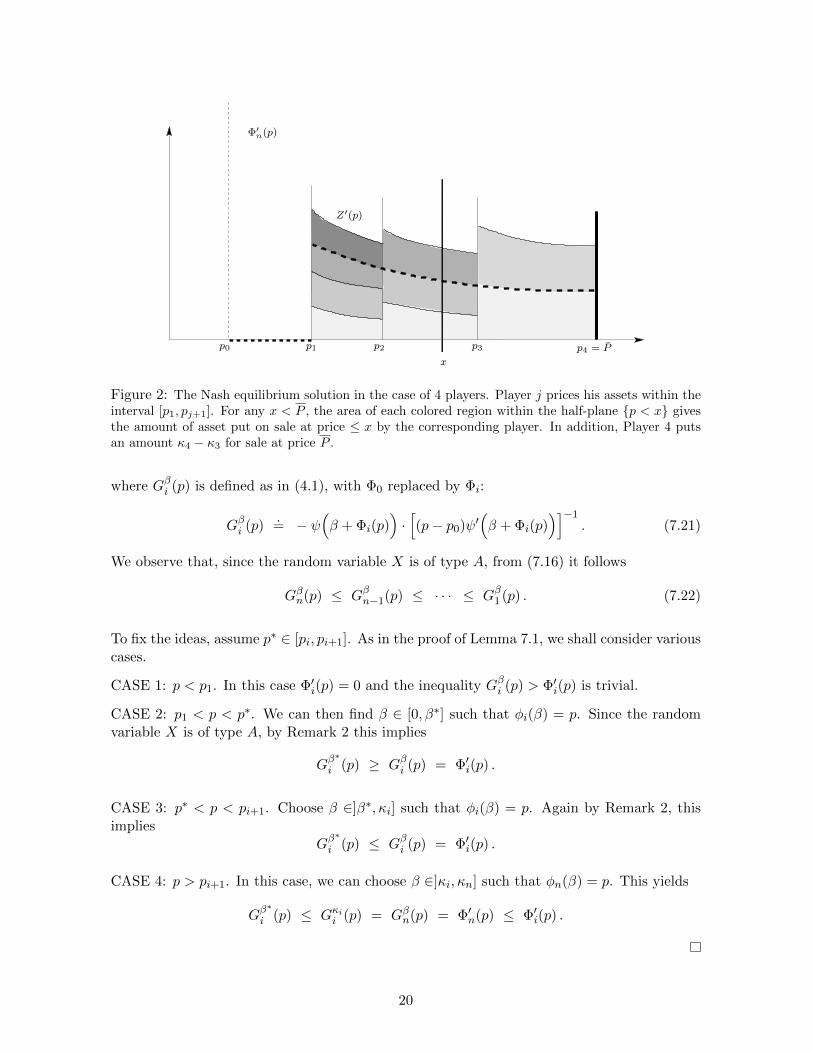
p0 p1 p2 p3 p4 = P

x

Z′(p)

Φ′n(p)

Figure 2: The Nash equilibrium solution in the case of 4 players. Player j prices his assets within theinterval [p1, pj+1]. For any x < P , the area of each colored region within the half-plane p < x givesthe amount of asset put on sale at price ≤ x by the corresponding player. In addition, Player 4 putsan amount κ4 − κ3 for sale at price P .

where Gβi (p) is defined as in (4.1), with Φ0 replaced by Φi:

Gβi (p).= − ψ

(β + Φi(p)

)·[(p− p0)ψ′

(β + Φi(p)

)]−1. (7.21)

We observe that, since the random variable X is of type A, from (7.16) it follows

Gβn(p) ≤ Gβn−1(p) ≤ · · · ≤ Gβ1 (p) . (7.22)

To fix the ideas, assume p∗ ∈ [pi, pi+1]. As in the proof of Lemma 7.1, we shall consider variouscases.

CASE 1: p < p1. In this case Φ′i(p) = 0 and the inequality Gβi (p) > Φ′i(p) is trivial.

CASE 2: p1 < p < p∗. We can then find β ∈ [0, β∗] such that φi(β) = p. Since the randomvariable X is of type A, by Remark 2 this implies

Gβ∗

i (p) ≥ Gβi (p) = Φ′i(p) .

CASE 3: p∗ pi+1. In this case, we can choose β ∈]κi, κn] such that φn(β) = p. This yields

Gβ∗

i (p) ≤ Gκii (p) = Gβn(p) = Φ′n(p) ≤ Φ′i(p) .

20

Theorem 7.3 (nonexistence of a Nash equilibrium). Let X be a random variable of typeB, satisfying the assumptions (A1). Then, for any number n ≥ 2 of players offering amountsκ1, . . . , κn > 0 of the same asset for sale, a Nash equilibrium cannot exist (regardless of theselling priorities established among the players).

Proof. 1. Assume, on the contrary, that a Nash equilibrium (φ∗1, . . . , φ∗n) exists. By Theorem

5.3, each pricing strategy φ∗i must be constant, say

φ∗i (β) ≡ pi, i = 1, . . . , n.

We claim thati 6= j =⇒ pi 6= pj .

Otherwise, since one of the two players does not have the priority over the other, he couldincrease his expected payoff by pricing all his asset at pi − ε, for some ε small enough.

2. Letε

.= min

i 6=j|pi − pj |.

Choose k ∈ 1, . . . , n such that pk < P . Then the k-th player can unilaterally increase hispayoff by using the strategy

φ∗k(β) = pk +ε

2.

This contradiction shows that no Nash equilibrium can exist.

8 Uniqueness of the Nash equilibrium

In this section we prove that, if the random variable X is of type A, then the Nash equilibriumconstructed in Theorem 7.2 is unique.

In the following, given an n-tuple of pricing strategies φ : [0, κi] 7→ [0, P ], we denote by

Fi(p).= sup

β ∈ [0, κi] ; φi(β) ≤ p

(8.1)

the amount of asset put on sale at price ≤ p by the i-th player. Moreover, we define

F (p) =n∑i=1

Fi(p).

Observe that, with these definitions, the functions Φi in (7.1) are expressed by

Φi(p) =∑j 6=i

Fj(p) = F (p)− Fi(p) .

Lemma 8.1. Let the n-tuple (φ1, . . . , φn) be a Nash equilibrium. Then the following holds.

(i) There exists a Lipschitz constant C such that

F (p2)− F (p1) ≤ C(p2 − p1) for all p0 < p1 < p2 < P . (8.2)

21

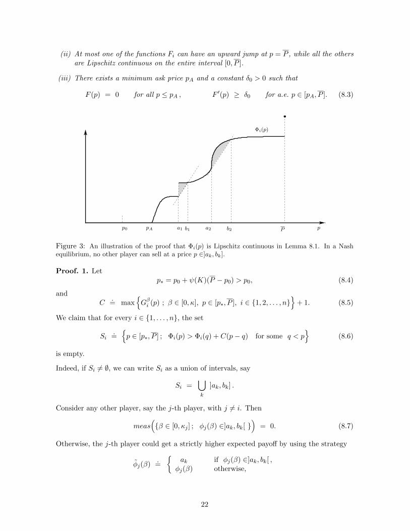
(ii) At most one of the functions Fi can have an upward jump at p = P , while all the othersare Lipschitz continuous on the entire interval [0, P ].

(iii) There exists a minimum ask price pA and a constant δ0 > 0 such that

F (p) = 0 for all p ≤ pA , F ′(p) ≥ δ0 for a.e. p ∈ [pA, P ]. (8.3)

p0 pA a1 b1 a2 b2 P p

Φi(p)

Figure 3: An illustration of the proof that Φi(p) is Lipschitz continuous in Lemma 8.1. In a Nashequilibrium, no other player can sell at a price p ∈]ak, bk].

Proof. 1. Letp∗ = p0 + ψ(K)(P − p0) > p0, (8.4)

andC

.= max

Gβi (p) ; β ∈ [0, κ], p ∈ [p∗, P ], i ∈ 1, 2, . . . , n

+ 1. (8.5)

We claim that for every i ∈ 1, . . . , n, the set

Si.=p ∈ [p∗, P ] ; Φi(p) > Φi(q) + C(p− q) for some q < p

(8.6)

is empty.

Indeed, if Si 6= ∅, we can write Si as a union of intervals, say

Si =⋃k

]ak, bk] .

Consider any other player, say the j-th player, with j 6= i. Then

meas(β ∈ [0, κj ] ; φj(β) ∈]ak, bk[

)= 0. (8.7)

Otherwise, the j-th player could get a strictly higher expected payoff by using the strategy

φj(β).=

ak if φj(β) ∈]ak, bk[ ,

φj(β) otherwise,

22

as the following computation shows:

J(φj)− J(φj) =

∫β ; φj(β)∈[ak,bk]

(ak − p0) · ψ(β + Φj(ak))− (φj(β)− p0) · ψ(β + Φj(φj(β))

≥∫β ; φj(β)∈[ak,bk]

∫ ak

φj(β)

d

dp

((p− p0)ψ (β + Φj(ak)− C(ak − p))

)dp dβ

≥ −∫β ; φj(β)∈[ak,bk]

∫ φj(β)

ak

(p− p0)ψ′ (β + Φj(ak)− C(ak − p)) ·

·

C − ψ(β + Φj(ak)− C(ak − p)

)(p− p0)ψ′

(β + Φj(ak)− C(ak − p)

) dp dβ

≥ −∫β ; φj(β)∈[ak,bk]

∫ φj(β)

ak

(p− p0)ψ′ (β + Φj(ak)− C(ak − p)) ·

· (C −Gβj (ak)) dp dβ > 0

The first inequality follows from (8.6) and the Fundamental Theorem of Calculus, the thirdinequality follows from the fact that X is of Type A, and the strict inequality follows fromthe definition (8.5).

However, if (8.7) holds for every j 6= i, then the strategy φi for the i-th player is not optimal.Indeed, he could achieve a strictly higher payoff by setting

φi(β).=

bk − ε if φi(β) ∈ [ak, bk[ ,φi(β) otherwise,

for some ε > 0 sufficiently small. This proves that Φj is Lipschitz on the interval [p∗, P ] forevery j ∈ 1, . . . , n. Since

F =1

n− 1

n∑j=1

Φj ,

we conclude that F is Lipschitz continuous on [p∗, P [.

Let p be a point such that F ′(p) > 0. Then at least one agent is putting some shares on saleat the price p. From the necessary conditions (4.28) on the best reply of any of the n players,if F ′ > 0, then it satisfies the inequality

F ′(p) ≥ Φ′j(p) =−ψ(F )

(p− p0)ψ′(F ), F (P ) ≤ K

.=

n∑i=1

κi p ∈ [p∗, P [.

Denote by Y (p) the solution to the terminal value problem

Y ′ =−ψ(Y )

(p− p0)ψ′(Y ), Y (P ) = K .

By direct computation we see that

ψ(Y (p)) =P − p0

p− p0ψ(K),

23

which implies that Y (p∗) = 0, where p∗ is given by (8.4). By comparison, we see thatY (p) ≥ F (p) and therefore

pA.= infp : F (p) > 0 ≥ p∗ > p0.

This proves the first assertion of the Lemma.

2. The second assertion is clear: if two players put a positive amount of asset for sale at thesame price P , the one that does not have priority can improve his expected payoff by sellingthe asset at price P − ε.

3. Toward a proof of (iii), we show that there exists δ0 > 0 small enough so that, for anyp∗ 0. By (i) it follows that F is differentiable at a.e. point p ∈ [0, P ].Assume F ′(p∗) ≤ δ0 and consider the non-empty set

S∗.=p < p∗ ; F (p) > F (p∗)− 2δ0(p∗ − p)

.

If F (p) = F (p∗) for all p ∈ S∗, recalling that F is Lipschitz continuous we conclude thatF (p) = F (p∗) = 0 for all p ≤ p∗, as claimed.

In the opposite case, there exist p′ < p∗ such that

F (p′) < F (p∗) , F (p) ≥ F (p∗)− 2δ0(p∗ − p) for all p ∈ [p′, p∗]. (8.9)

Clearly, at least one the the players is putting some assets for sale within the price interval[p′, p∗], say, the i-th player. This leads to a contradiction, because by (8.9)

Φi(p) ≥ Φi(p∗)− 2δ0(p∗ − p) ,

Hence the strategy

φi(β) =

p∗ if φi(β) ∈ [p′, p∗] ,

φi(β) otherwise ,

yields a strictly higher expected payoff:

J(φi)− J(φi) =

∫β ; φi(β)∈[p′,p∗]

∫ p∗

φi(β)(p− p0)ψ′ (β + Φi(p)) ·

(Φ′i(p)−G

βi (p)

)dp dβ

≥∫β ; φj(β)∈[p′,p∗]

∫ p∗

φj(β)(p− p0)ψ′ (β + Φi(p)) ·

(2δ0 −Gβi (p)

)dp dβ > 0 .

24

p0 pA p′ p∗ P p

Φi(p)

Figure 4: If Φ′i ≤ F ′ is small, then the i-th player can improve his expected payoff by asking thehigher price p∗ instead of a price p ∈ [p′, p∗].

Theorem 8.2. In the same setting of Theorem 7.2, the Nash equilibrium is unique.

Proof. 1. Let (φ1, . . . , φn) be a Nash equilibrium. By Lemma 8.1, the corresponding func-tions Fi are Lipschitz continuous on [0, P [ , and all except at most one of them are Lipschitzcontinuous on the closed interval [0, P ]. Moreover, there exists a minimum ask price pA suchthat (iii) in Lemma 8.1 holds.

2. By Rademacher’s theorem, every function Fi is differentiable a.e. on [0, P [ . For each p,consider the set of indices

I(p).= i ; F ′(p) > 0

and call N(p).= #I(p) the cardinality of this set. By Lemma 8.1 the function N(·) is well

defined and Lebesgue measurable. Moreover, N(p) ≥ 2 for a.e. p ∈ [pA, P ].

For p ∈ [pA, P [, i ∈ I(p), let βi ∈ [0, κi] be such that φi(βi) = p. Recalling (4.1), from thenecessary conditions (4.9) we deduce

Φ′i(p) = Gβii (p) =−ψ(F (p))

(p− p0)ψ′(F (p))i ∈ I(p) .

Observing that

Φ′i(p) =∑j 6=i

F ′j(p),

one obtainsΦ′i(p) =

N(p)− 1

N(p)F ′(p) , F ′i (p) =

F ′(p)

N(p)for i ∈ I(p) ,

Φ′i(p) = F ′(p), F ′i (p) = 0 for i /∈ I(p) .

The Lipschitz function F thus satisfies the ODE

F ′(p) =N(p)

N(p)− 1· −ψ(F (p))

(p− p0)ψ′(F (p))(8.10)

25

at a.e. point p ∈ [pA, P ].

pA p1 p′ p2 p pA p1 p′ p2 p

γ2(p)

γ1(p)

Φi(p)

γ2(p)

γ1(p)

Φi(p)

Figure 5: A graph of the function Φi. If player i sells something at price p2 but nothing at price p1,then his strategy is not optimal. Left: Case 1. Right: Case 2.

3. We claim that, for each i ∈ 1, . . . , n, the set of prices where the i-th player offers assetsfor sale is an interval [pA, pi+1]. Assume, on the contrary, that this is not the case. To derivea contradiction, call

Si.= p ∈ [p0, P ] ; F ′i > 0

andLi

.= p ∈ [p0, P ] ; p is a Lebesgue point of F ′i .

Letq ∈

([pA, P ] ∩ Li

)\ Si

and assume that[q, P ] ∩ Li ∩ Si 6= ∅. (8.11)

Letq∗

.= inf[q, P ] ∩ Li ∩ Si.

Then, for any δ1 > 0, the following two sets are non-empty:

A.= ([q∗ − δ1, q

∗] ∩ Li) \ Si 6= ∅, B.= [q∗, q∗ + δ1] ∩ Li ∩ Si 6= ∅.

Indeed, B is nonempty, by the definition of infimum. Moreover, if q∗ = q then q∗ ∈ A 6= ∅,otherwise A is nonempty by the definition of infimum.

From the necessary conditions (4.28) we deduce

Φ′i(p) = F ′(p) =N(p)

N(p)− 1· −ψ(F (p))

(p− p0)ψ′(F (p))≥ n

n− 1· −ψ(F (p))

(p− p0)ψ′(F (p))

for p /∈ Si, while

Φ′i(p) =−ψ(F (p))

(p− p0)ψ′(F (p))

for p ∈ Si.

26

Choose the intermediate slope

λ.=

(2n− 1

2n− 2

)−ψ(F (q∗))

(q∗ − p0)ψ′(F (q∗)). (8.12)

By continuity we can choose δ0 < δ1 small enough so that

λ− −ψ(F (p))

(p− p0)ψ′(F (p))> 0, for all p ∈ [q∗ − δ0, q

∗ + δ0].

Finally, let p1 ∈ A and p2 ∈ B be Lebesgue points of F ′i and consider the two lines

γ1(p) = Φi(p1) + λ(p− p1) , γ2(p) = Φi(p2) + λ(p− p2) .

We split the analysis into two cases (Fig. 5).

CASE 1: γ1 ≥ γ2. We then consider the intermediate point

p′.= min

p > p1 ; Φi(p) = γ1(p)

.

Observe that p′ > p1, because p1 ∈ Li \ Si and Φ′i(p1) > λ.

Then the new pricing strategy

φi(β) =

p1 if φi(β) ∈ [p1, p

′] ,φi(β) otherwise,

yields a strictly better expected payoff:

J(φi)− J(φi) =

∫β ; φi(β)∈[p1,p′]

(p1 − p0) · ψ(β + Φi(p1))− (φi(β)− p0) · ψ(β + Φi(φi(β))

≥∫β ; φi(β)∈[p1,p′]

∫ p1

φi(β)

d

dp

((p− p0)ψ (β + γ1(p))

)dp dβ

= −∫β ; φi(β)∈[p1,p′]

∫ φi(β)

p1

(p− p0)ψ′ (β + Φi(p)) ·

·

λ− ψ(β + γ1(p)

)(p− p0)ψ′

(β + γ1(p)

) dp dβ > 0.

CASE 2: γ1 < γ2. We then consider the intermediate point

p′.= maxp < p2 ; Φi(p) = γ2(p) .

An entirely similar argument now shows that the new pricing strategy

φi(β) =

p′ if φi(β) ∈ [p′, p2] ,

φi(β) otherwise,

27

yields a strictly better expected payoff.In both cases we showed that φi is not optimal, thus reaching a contradiction.

4. From the previous step it follows

p1 ≤ p2 ≤ · · · ≤ pn ≤ pn+1 ≤ P .

We claim that pn = pn+1 = P .

Indeed, if pn < pn+1, this means that the n-th player is the only seller in the interval [pn, pn+1].He could achieve a better expected payoff by taking all his assets originally on sale at a pricep ∈ [pn, pn+1] and offering them at the price pn+1 instead. This shows that pn = pn+1.

Finally we show that pn = P . Indeed, if this were not the case, we would have

F ′(p) = 0, for all p ∈ ]pn, P ] ,

contradicting the third statement in Lemma 8.1.

9 A large number of small agents

In this section we study the limiting case where the number of sellers approaches infinity, butthe total amount of asset offered for sale remains bounded.

Example 3. Consider the simple case of n players, each one selling the same amount K/n ofasset. By (7.7) in the proof of Lemma 7.1, the total amount Zn(p) = n

n−1Φ(p) of asset put onsale at price ≤ p is found by solving the ODE

n− 1

nZ ′n =

−ψ(Zn(p))

(p− p0)ψ′(Zn), Zn(P ) = K .

As n→∞, the limit distribution Z(p) = limn→∞ Zn(p) is clearly obtained by solving

Z ′ =−ψ(Z)

(p− p0)ψ′(Z), Z(P ) = K . (9.1)

We wish to show that the same limit holds, without assuming that all players put on saleexactly the same amount of asset. Consider a sequence of bidding games, satisfying:

(G1) The n-th game involves n distinct players, selling the amounts κn,1, . . . , κn,n of the sameasset.

(G2) The total amount of asset put on sale in the n-th game is Kn.=∑n

i=1 κn,i, withlimn→∞Kn = K.

(G3) The largest amount of asset put on sale by any player in the n-th game approacheszero: limn→∞

(sup1≤i≤n κn,i

)= 0.

28

The next result shows that, with the above assumptions, as n → ∞ the limit order bookapproaches a well defined shape. In the following, we call Zn(p) the amount of asset offeredfor sale at price < p, in the Nash equilibrium solution (7.15) for the n-th game. Moreover, welet Z(p) to be the solution to the Cauchy problem (9.1).

Observe that the right hand side of the ODE in (9.1) is well defined and uniformly positive aslong as Z ∈ [0,K]. Indeed,

Z ′(p) ≥ C0

p− p0

for some constant C0 > 0. By a comparison argument we conclude that there exists a valuepA > p0 such that the solution of (9.1) satisfies

Z(pA) = 0 , Z(p) > 0 for pA < p < P . (9.2)

We then extend the function Z to the entire interval [0, P ] by setting

Z(p).= 0 for p ∈ [0, pA] . (9.3)

Theorem 9.1. Let X be a random variable of type A, satisfying the assumptions (A1). Con-sider a sequence of games for n players, satisfying (G1)–(G3).

Then, for any ε > 0, the following holds.

limn→∞

Zn(p) = Z(p) uniformly for all p ∈ [0, P ] , (9.4)

limn→∞

Z ′n(p) = Z ′(p) uniformly for all p ∈ [0, pA − ε] ∪ [pA + ε , P − ε] , (9.5)

where Z is defined by (9.1), (9.3), and pA is determined by (9.2).

Proof. 1. For a given n ≥ 1, it is not restrictive to assume κn,1 ≤ κn,2 ≤ · · · ≤ κn,n. For1 < i ≤ n call hn,i

.= κn,i−κn,i−1. Moreover, set hn,1

.= κn,1. In the Nash equilibrium solution

for the n-th game, the total amount Zn(p) put on sale at price < p is characterized by theequations

Zn(P ) = Kn − hn,n , Zn(p) = 0 for p ∈ [0, pn,1] , (9.6)

Z ′n(p) =n− i+ 1

n− i· −ψ(Zn(p))

(p− p0)ψ′(Zn(p))for pn,i 0, ψ′ < 0, from (9.7) we deduce

−ψ(Zn(p))

(p− p0)ψ′(Zn(p))≤ Z ′n(p) ≤ −2ψ(Zn(p))

(p− p0)ψ′(Zn(p)), pn,1 < p < P, (9.9)

−ψ(Zn(p))

(p− p0)ψ′(Zn(p))≤ Z ′n(p) ≤ −(m+ 1)

m

ψ(Zn(p))

(p− p0)ψ′(Zn(p))for pn,n−m < p < P .

(9.10)

29

2. For any fixed m ≥ 1, we claim that

pn,n−m → P , Zn(pn,n−m) → K as n→∞. (9.11)

Indeed, by (9.9) it follows that all maps Zn(·) are increasing and uniformly Lipschitz contin-uous, say

Zn(P )− C(P − p) ≤ Zn(p) ≤ Zn(P ) for all p ∈[pA + P

2, P

], (9.12)

for some Lipschitz constant C. Since Zn(P ) = Kn − hn → K as n → ∞, we can find δ > 0such that

K

2≤ Zn(p) ≤ 2K for all p ∈ [P − δ, P ] (9.13)

and all n sufficiently large. By (9.8) one has∫ P

pn,n−m

Z ′n(p) dp ≤ (m+ 1) ·n−1∑

i=n−m

∫ pn,i+1

pn,i

Z ′n(p)

n− i+ 1dp = (m+ 1)

n∑i=n−m

hn,i−1

≤ (m+ 1) (κn,n−1 − κn−m−1) ≤ (m+ 1)κn,n → 0

(9.14)

as n → ∞. Together, (9.13) and (9.14) imply (9.11). Indeed, using (9.10), (9.13) and theassumption (A1), it follows that, if pn,n−m 0.

By (9.14) we thus have pn,n−m ≥ P − δ for all n sufficiently large. Therefore

K

2· (P − pn,n−m) ≤

∫ P

pn,n−m

Z ′n(p) dp → 0,

showing that pn,n−m → P as n→∞. In turn, this implies

|Zn(pn,n−m)−K| ≤ |Zn(pn,n−m)− Zn(P )|+ |Zn(P )−K|

≤ C(P − pn,n−m) + |K −Kn|+ κn,n → 0.

3. By the previous step, the function Zn satisfies the differential inequalities

−m+ 1

m

ψ(Zn(p))

(p− p0)ψ′(Zn(p))≤ Z ′n(p) ≤ −ψ(Zn(p))

(p− p0)ψ′(Zn(p)), pn,1 < p < pn,n−m, (9.15)

with terminal conditions at p = pn,n−m satisfying (9.11). We now compare (9.15) and (9.11)with (9.1). By standard results on the continuous dependence of solutions to a Cauchy prob-lem, for any ε > 0 we have the convergence (see Fig. 6)

Zn(p) → Z(p), Z ′n(p) → Z ′(p), (9.16)

30

Zn(p)

Z(p)

pA+εpA

p1,np0 PP−ε

K

Figure 6: On any subinterval [pA + ε, P − ε] we have the uniform convergence Zn(p) → Z(p). Sinceeach derivative Z ′n is uniformly positive on the region where Zn > 0, this implies the convergencepn → pA.

uniformly on the interval [pA + ε, P − ε].

By (9.9), on the region where Zn > 0 the derivative satisfies Z ′n(p) ≥ c0 for some constantc0 > 0 and all p > 0, n ≥ 2. Since in (9.16) we can choose ε > 0 arbitrarily small, we concludethat the value pn in (9.6) satisfy

limn→∞

pn,1 = pA (9.17)

Observing thatZn(p) = 0 for p ∈ [0, pn,1] ,Z(p) = 0 for p ∈ [0, pA] ,

and that all functions Z,Zn are uniformly Lipschitz continuous, from (9.16) and (9.17) wededuce the convergence (9.4)-(9.5).

10 Examples

In this section we consider in more detail the case when the probability distribution of size ofincoming market order is given by (2.5) or (2.6).

Example 4. Assume that the size of the incoming market order is exponentially distributed,with mean λ−1. Two competing agents put on sale the amounts κ1 < κ2 of shares. The Nashequilibrium (7.15) is given by

φ∗2(β) =

p0 + e−λκ1+λβ · [P − p0], β ∈ [0, κ1] ,

P β ∈ [κ1, κ2] ,

φ∗1(β) = p0 + e−λκ1+λβ · [P − p0], β ∈ [0, κ1] .

(10.1)

31

The cumulative limit order book is thus given by

F (p) =

0 p ∈ [p0, pA[,2

λln

(p− p0)

P − p0

p ∈ [pA, P [,

κ1 + κ2 p = P .

This corresponds to a limit order book density

F ′(p) =2

λ(p− p0)χ[pA,P ](p) + (κ2 − κ1) · δP ,

where δP denotes a unit Dirac mass located at p = P , and the ask price pA is given by

pA = p0 + (P − p0) · e−λκ1 .

The expected payoffs of the two agents in the Nash equilibrium configuration are given by

J1 =

∫ κ1

0(φ∗1(β)− p0) · e−2λβ dβ =

e−λκ1(1− e−λκ1)(P − p0)

λ

J2 = J1 + E[(X − κ1)+ ∧ κ2] =e−λκ1(1− e−λ(κ2+2κ1))(P − p0)

λ.

We observe that an increase in the total amount put on sale by the smaller player (hence byboth players) lowers the ask price, and also decreases the expected payoff of both competitors.

J1, J2 0, as κ1 →∞.

On the other hand, the larger player can increase his expected payoff by increasing the totalamount of shares he puts on sale:

J2 e−λκ1(P − p0)

λ, as κ2 →∞, κ1 fixed.

Finally, using the explicit expression of the limit order book resulting from the Nash equilib-rium, we can also derive an expression for the price impact function ρ(X), which representsthe increase in the ask price in response to a market order of size X. Indeed, ρ(X) is definedby the following implicit equation

Z(pA + ρ(X)) = Z(pA) +X . (10.2)

This yields

ρ(X) =

(e

λX2 − 1)(P − p0)e−λκ1 if X ≤ 2κ1 ,

P − pA if X > 2κ1 .

Example 5. Consider the asymptotic limit of a large number of small agents, putting on sale atotal amount of K shares. Assume that the size of the incoming market order is exponentiallydistributed, as in (2.5). In this case, the Cauchy problem (9.1) simplifies to

Z ′(p) =1

λ(p− p0), Z(P ) = K .

32

The expected payoff per unit amount of asset put on sale by any agent is given by

Ju = (P − p0)e−λK

The ask price is pA = p0 + (P − p0) · e−λK , while the price impact function is given by

ρ(X) =

(eλX − 1)(P − p0)e−λK if X ≤ K ,

P − pA if X > K .

Example 6. Assume that the random size X of the incoming buying order is distributedaccording to the power law distribution (2.6). Consider n players, each one putting on salethe same amount κ of shares, for a total amount of K = nκ.

The Nash equilibrium is thus given by (7.4):

φ∗1(β) = · · · = φ∗n(β) = φ(β).= p0 + [P − p0] ·

(1 + nβ

1 + nκ

)n−1n

α

,

and the corresponding ask price is

pnA = φ(0) = p0 + [P − p0] · (1 + nκ)1−nn

α .

The cumulative limit order book is thus given by

Zn(p) = (1 + nκ)(P − p0

)− 1α

nn−1 · (p− p0)

1α

nn−1 − 1, p ∈ [pnA, P ].

The corresponding order book density is then

Z ′n(p) =n

α(n− 1)· (1 + nκ)

(P − p0

)− 1α

nn−1 · (p− p0)

n(1−α)+αnα−α , p ∈ [pnA, P ].

From the above expressions we can easily compute the asymptotic limit as the number ofplayers goes to infinity, for K = nκ fixed. The ask price is pA = p0 + [P − p0] · (1 +K)−α andthe shape of the limit order book is given by

Z(p) = (1 +K)(P − p0

)− 1α · (p− p0)

1α − 1, p ∈ [pA, P ] ,

Z ′(p) =1

α· (1 +K)

(P − p0

)− 1α · (p− p0)

1−αα , p ∈ [pA, P ].

In this case, the price impact function is given by

ρ(X) =P − p0

(1 +K)α· [(1 +X)α − 1], X ≤ K.

33

References

[1] A. Alfonsi, A. Fruth and A. Schied, Optimal execution strategies in limit order bookswith general shape functions, Quantitative Finance 10 (2010), 143-157.

[2] M. Avellaneda and S. Stoikov, High-frequency trading in a limit order book, QuantitativeFinance 8 (2008), 217-224.

[3] A. Bressan, Noncooperative differential games. Milan J. of Mathematics, 79 (2011), 357-427.

[4] L. Cesari, Optimization Theory and Applications. Springer-Verlag, 1983.

[5] R. Cont, S. Stoikov, and R. Talreja, A stochastic model for order book dynamics, Oper-ations Research 58 (2010), 549-563.

[6] E. J. Dockner, S. Jorgensen, N. V. Long, and G. Sorger, Differential games in economicsand management science. Cambridge University Press, 2000.

[7] J. Nash, Non-cooperative games, Annals of Math. 2 (1951), 286-295.

[8] A. Obizhaeva, and J. Wang, Optimal trading strategy and supply/demand dynamics,Journal of Financial Markets, to appear.

[9] T. Preis, S. Golke, W. Paul, and J. J. Schneider, Multi-agent-based order book model offinancial markets. Europhysics Letters 75 (2006), 510-516.

[10] S. Predoiu, G. Shaikhet, and S. Shreve, Optimal execution in a general one-sided limit-order book. SIAM Journal on Financial Mathematics 2 (2010), 183-212.

[11] A. N. Kolmogorov and S. V. Fomin, Introductory Real Analysis. Dover Publications, NewYork, 1970.

[12] I. Rosu, A dynamic model of the limit order book. The Review of Financial Studies 22(2009), 4601-4641.

[13] N. Vorob’ev, Foundations of game theory. Noncooperative games. Birkhauser, Basel, 1994.

[14] J. Wang, The Theory of Games. Oxford University Press, 1988.

34

optimal pricing strategies in a continuum limit order book pricing strategies in a continuum limit...

Documents