Optimal Power Allocation in Server Farms

Anshul Gandhi∗ Mor Harchol-Balter∗Rajarshi Das† Charles Lefurgy††

March 2009CMU-CS-09-113

School of Computer ScienceCarnegie Mellon University

Pittsburgh, PA 15213

∗School of Computer Science, Carnegie Mellon University, Pittsburgh, PA, USA†IBM T.J. Watson Research Center, Hawthorne, NY, USA††IBM Research, Austin, TX, USA

Research supported by NSF SMA/PDOS Grant CCR-0615262 and a 2009 IBM Faculty Award.The views and conclusions contained in this document are those of the authors and should not be interpreted asrepresenting the official policies, either expressed or implied, of NSF or IBM.

Keywords: Power Management, Server Farm, Response Time, Power-to-Frequency, DataCenter

Abstract

Server farms today consume more than 1.5% of the total electricity in the U.S. at a cost of nearly$4.5 billion. Given the rising cost of energy, many industries are now looking for solutions on howto best make use of their available power. An important question which arises in this context ishow to distribute available power among servers in a server farm so as to get maximum perfor-mance. By giving more power to a server, one can get higher server frequency (speed). Henceit is commonly believed that for a given power budget, performance can be maximized by oper-ating servers at their highest power levels. However, it is also conceivable that one might preferto run servers at their lowest power levels, which allows more servers for a given power budget.To fully understand the effect of power allocation on performance in a server farm with a fixedpower budget, we introduce a queueing theoretic model, which also allows us to predict the opti-mal power allocation in a variety of scenarios. Results are verified via extensive experiments on anIBM BladeCenter. We find that the optimal power allocation varies for different scenarios. In par-ticular, it is not always optimal to run servers at their maximum power levels. There are scenarioswhere it might be optimal to run servers at their lowest power levels or at some intermediate powerlevels. Our analysis shows that the optimal power allocation is non-obvious, and, in fact, dependson many factors such as the power-to-frequency relationship in the processors, arrival rate of jobs,maximum server frequency, lowest attainable server frequency and server farm configuration. Fur-thermore, our theoretical model allows us to explore more general settings than we can implement,including arbitrarily large server farms and different power-to-frequency curves. Importantly, weshow that the optimal power allocation can significantly improve server farm performance, by afactor of typically 1.4 and as much as a factor of 5 in some cases.

1 IntroductionServers today consume ten times more power than they did ten years ago [3, 19]. Recent articlesestimate that a 300W high performance server requires more than $330 of energy cost per year [22].Given the large number of servers in use today, the worldwide expenditure on enterprise power andcooling of these servers is estimated to be in excess of $30 billion [19].

Power consumption is particularly pronounced in CPU intensive server farms composed oftens to thousands of servers, all sharing workload and power supply. We consider server farmswhere each incoming job can be routed to any server, i.e., it has no affinity for a particular server.

Server farms usually have a fixed peak power budget. This is because large power consumersoperating server farms are often partly billed by power suppliers based on their peak power require-ments. The peak power budget of a server farm also determines it’s cooling and power deliveryinfrastructure costs. Hence, companies are interested in maximizing the performance at a serverfarm given a fixed peak power budget [4, 8, 19, 24].

The power allocation problem we consider is: how to distribute available power among serversin a server farm so as to minimize mean response time. Every server running a given workload hasa minimum level of power consumption, b, needed to operate the processor at the lowest allowablefrequency and a maximum level of power consumption, c, needed to operate the processor at thehighest allowable frequency. By varying the power allocated to a server within the range of b to cWatts, one can proportionately vary the server frequency (See Fig. 2(a) and (b)). Hence, one mightexpect that running servers at their highest power levels of c Watts, which we refer to as PowMax,is the optimal power allocation scheme to minimize response time. Since we are constrained bya power budget, there are only a limited number of servers that we can operate at highest powerlevels. The rest of the servers remain turned off. Thus PowMax corresponds to having few fastservers. In sharp contrast is PowMin, which we define as operating servers at their lowest powerlevels of b Watts. Since we spend less power on each server, PowMin corresponds to having manyslow servers. Of course there might be scenarios where we neither operate our servers at the highestpower levels nor at the lowest power levels, but we operate them at some intermediate power levels.We refer to such power allocation schemes as PowMed.

Understanding power allocation in a server farm is intrinsically difficult for many reasons:First, there is no single allocation scheme which is optimal in all scenarios. For example, it iscommonly believed that PowMax is the optimal power allocation scheme [1, 7]. However, aswe show later, PowMin and PowMed can sometimes outperform PowMax by almost a factor of1.5. Second, it turns out that the optimal power allocation depends on a very long list of externalfactors, such as the outside arrival rate, whether an open or closed workload configuration is used,the power-to-frequency relationship (how power translates to server frequency) inherent in thetechnology, the minimum power consumption of a server (b Watts), the maximum power that aserver can use (c Watts), and many other factors. It is simply impossible to examine all theseissues via experiments.

To fully understand the effect of power allocation on mean response time in a server farmwith a fixed power budget, we introduce a queueing theoretic model, which allows us to predictthe optimal power allocation in a variety of scenarios. We then verify our results via extensiveexperiments on an IBM BladeCenter.

1

Low arrival rate High arrival rate0

5

10

15

20

25

30

35

40

45

50

Mean r

esponse tim

e (

sec)

→

PowMinPowMax

PowMax beats PowMinPowMax beats PowMin

Low arrival rate High arrival rate0

5

10

15

20

25

30

35

40

45

50

Me

an

re

sp

on

se

tim

e (

se

c)

→

PowMinPowMax

PowMin beats PowMax

PowMax beats PowMin

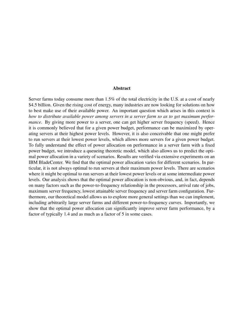
(a) PowMax is best. (b) PowMin is best (c) PowMed is bestat high arrival rates. at high arrival rates.

Figure 1: Subset of our results, showing that no single power allocation scheme is optimal.Fig.(a) depicts a scenario using DFS where PowMax is optimal. Fig.(b) depicts a scenario usingDVFS where PowMin is optimal at high arrival rates whereas PowMax is optimal at low arrivalrates. Fig.(c) depicts a scenario using DVFS+DFS where PowMed is optimal at high arrival rateswhereas PowMax is optimal at low arrival rates.

Prior work in power management has been motivated by the idea of managing power at theglobal data center level rather than at the more localized single-server level [24, 18]. While powermanagement in server farms deals with various issues such as reducing cooling costs, minimiz-ing idle power wastage and minimizing average power consumption, we are more interested inthe problem of allocating peak power among servers in a server farm to maximize performance.Notable prior work dealing with peak power allocation in a server farm includes Raghavendraet al. [19], Femal et al. [9] and Chase et al. [5] among others. Raghavendra et al. [19] presenta power management solution that coordinates different individual approaches to simultaneouslyaddress the issues listed above. Femal et al. [9] allocate peak power so as to maximize throughputin a data center while simultaneously attempting to satisfy certain operating constraints such asload-balancing the available power among the servers. Chase et al. [5] present an auction-basedarchitecture for improving the energy efficiency of data centers while achieving some quality-of-service specifications. We differ from the above work in that we specifically deal with minimizingmean response time for a given peak power budget and understanding all the factors that affect it.

Our contributionsAs we have stated, the optimal power allocation scheme depends on many factors. Perhaps themost important of these is the specific relationship between the power allocated to a server andit’s frequency (speed), henceforth referred to as the power-to-frequency relationship. There areseveral mechanisms within processors that control the power-to-frequency relationship. These canbe categorized into DFS (Dynamic Frequency Scaling), DVFS (Dynamic Voltage and FrequencyScaling) and DVFS+DFS. Section 2 discusses these mechanisms in more detail. The functionalform of the power-to-frequency relationship for a server depends on many factors such as the

2

workload used, maximum server power, maximum server frequency and the voltage and frequencyscaling mechanism used (DFS, DVFS or DVFS+DFS). Unfortunately, the functional form of theserver level power-to-frequency relationship is only recently beginning to be studied (See the 2008papers [19, 23]) and is still not well understood. Our first contribution is the investigation of howpower allocation affects server frequency in a single server using DFS, DVFS and DVFS+DFSfor various workloads. In particular, in Section 3 we derive a functional form for the power-to-frequency relationship based on our measured values (See Figs. 2(a) and (b)).

Our second contribution is the development of a queueing theoretic model which predictsthe mean response time for a server farm as a function of many factors including the power-to-frequency relationship, arrival rate, peak power budget etc. The queueing model also allows us todetermine the optimal power allocation for every possible configuration of the above factors (SeeSection 4).

Our third contribution is the experimental implementation of our schemes, PowMax, PowMin,and PowMed, on an IBM BladeCenter, and the measurement of their response time for variousworkloads and voltage and frequency scaling mechanisms (See Sections 5 and 6). Importantly, ourexperiments show that using the optimal power allocation scheme can significantly reduce meanresponse times, sometimes by as much as a factor of 5. To be more concrete, we show a subsetof our results in Fig. 1, which assumes a CPU bound workload in an open loop setting. Fig. 1(a)depicts one possible scenario using DFS where PowMax is optimal. By contrast, Fig. 1(b) depictsa scenario using DVFS where PowMin is optimal for high arrival rates. Lastly, Fig. 1(c) depicts ascenario using DVFS+DFS where PowMed is optimal for high arrival rates.

We experiment with different workloads. While Section 5 presents experimental results fora CPU bound workload, LINPACK, Section 6 repeats all the experiments under other workloads,including the STREAM memory bound workload, the WebBench web-workload, and others. In allcases, experimental results are in excellent agreement with our theoretical predictions. Section 7summarizes our work. Finally, Section 8 discusses future applications of our model to more com-plex situations such as workloads with varying arrival rates, servers with idle (low power) statesand power management at the subsystem level, such as the storage subsystem.

2 Experimental framework

2.1 Experimental setupOur experimental setup consists of a server farm with up to fourteen IBM BladeCenter HS21 bladeservers featuring two 3.0 GHz dual-core Intel Woodcrest Xeon processors and 1 GB memoryper blade, all residing in a single chassis. We installed and configured Apache as an applicationserver on each of the blade servers to process transactional requests. To generate HTTP requestsfor the Apache web servers, we employ an additional blade server on the same chassis as theworkload generator to reduce the effects of network latency. The workload generator uses the webserver performance benchmarking tool httperf [17] in the open server farm configuration andwbox [21] in the closed server farm configuration. We modified and extended httperf andwbox to allow for multiple servers and to specify the routing probability among the servers. We

3

measure and allocate power to the servers using IBM’s Amester software. Amester along withadditional scripts collects all relevant data for our experiments.

2.2 Voltage and frequency scaling mechanismsProcessors today are commonly equipped with mechanisms to reduce power consumption at theexpense of reduced server frequency. Common examples of these mechanisms are Intel’s Speed-Step Technology and AMD’s Cool ’n’ Quiet Technology. The power-to-frequency relationship insuch servers depends on the specific voltage and frequency scaling mechanism used. Most mech-anisms fall under the following three categories:

Dynamic Frequency Scaling (DFS) a.k.a. Clock Throttling or T-states is a technique tomanage power by running the processor at a less-than-maximum clock frequency. Under DFS,the Intel’s 3.0 GHz Woodcrest Xeon processors we use allow for 8 operating points which corre-spond to effective frequencies of 12.5%, 25%, 37.5%, 50%, 62.5%, 75%, 87.5% and 100% of themaximum server frequency.

Dynamic Voltage and Frequency Scaling (DVFS) a.k.a. P-states is a more efficient power-savings mechanism that reduces server frequency by reducing the processor voltage and frequency.Under DVFS, our processors allow for 4 operating points which correspond to effective frequencies66.6%, 77.7%, 88.9%, and 100% of the maximum server frequency.

DVFS+DFS attempts to leverage both DVFS and DFS by applying DFS on the lowest perfor-mance state available in DVFS. Under DVFS+DFS, our processors allow for 11 operating pointswhich correspond to effective frequencies of 8.3%, 16.5%, 25%, 33.3%, 41.6%, 50.0%, 58.3%,66.6%, 77.7%, 88.9%, and 100% of the maximum server frequency.

2.3 Power consumption within a single serverWhen allocating power to a server, there is a minimum level of power consumption (b) needed tooperate the processor at the lowest allowable frequency and a maximum level of power consump-tion (c) needed to operate the processor at the highest allowable frequency (Of course the specificvalues of b and c depend on the application that the server is running). Formally, we define thefollowing notation:

Baseline power: b Watts The minimum power consumed by a fully-utilized server over theallowable range of processor frequency.Speed at baseline: sb Hertz The speed (or frequency) of a fully utilized server running at b Watts.Maximum power: c Watts The maximum power consumed by a fully-utilized server over theallowable range of processor frequency.Speed at maximum power: sc Hertz The speed (or frequency) of a fully utilized server runningat c Watts.

4

3 Power-to-frequencyAn integral part of determining the optimal power allocation is to understand the power-to-frequencyrelationship. This relationship differs for DFS, DVFS and DVFS+DFS, and also differs based onthe workload in use. Unfortunately, the functional form of the power-to-frequency relationshipis not well studied in the literature. The servers we use support all three voltage and frequencyscaling mechanisms and therefore can be used to study the power-to-frequency relationships. Inthis section, we present our measurements depicted in Figs. 2(a) and (b) showing the functionalrelationship between power allocated to a server and it’s frequency for the LINPACK [11] work-load. We generalize the functional form of the power-to-frequency relationship to other workloadsin Section 6 (See Figs. 8 and 10). Throughout we assume a homogeneous server farm.

We use the tools developed in [15] to limit the maximum power allocated to each server. Limit-ing the maximum power allocated to a server is usually referred to as capping the power allocatedto a server. We use LINPACK jobs with no inter-arrival time between them to ensure that the serveris always occupied by the workload. By running jobs back-to-back, we ensure that the server isrunning at the specified power cap value. Hence, the power values we observe will be the peakpower values for the specified workload. Recall from Section 2 that the voltage and frequencyscaling mechanisms have certain discrete performance points (in terms of frequency) at which theserver can operate. At each of these performance points, the server consumes a certain amount ofpower for a given workload. By quickly dithering between available performance states, we canensure that the server never consumes more than the set power cap value. In this way, we alsoget the best performance from the server for the given power cap value. Note that when we saypower, we mean the system-level power which includes the power consumed by the processor andall other components within the server.

Fig. 2(a) illustrates the power-to-frequency curves obtained for LINPACK using DFS andDVFS. From the figure, we see that the power-to-frequency relationship for both DFS and DVFS isalmost linear. It may seem surprising that the power-to-frequency relationship for DVFS looks likea linear plot. This is opposite to what is widely suggested in the literature for the processor power-to-frequency relationship, which is cubic [10]. The reason why the server power-to-frequencyrelationship is linear can be explained by two interrelated factors. First, manufacturers usuallysettle on a limited number of allowed voltage levels (or performance states), which results in less-than-ideal relationship between power and frequency in practice. Second, DVFS is not applied onmany components at the system level. For example, power consumption in memory remains pro-portional to the number of references to memory per unit time, which is only linearly related to thefrequency of the processor. Thus, the power-to-frequency curve for both DFS and DVFS can beapproximated as a linear function. Using the terminology introduced in Section 2, we approximatethe speed (or frequency) of the server, s GHz, as a function of the power allocated to it, P Watts,as:

s = sb + α(P − b). (1)

where the coefficient α (units of GHz per Watt) is the slope of the power-to-frequency curve.Specifically, our experiments show that α = 0.008 GHz/W for DVFS and α = 0.03 GHz/W forDFS. Also, from our experiments, we found that b = 180W and c = 240W for both DVFS and

5

(a) DFS and DVFS (b) DVFS+DFS

Figure 2: Power-to-frequency curves for DFS, DVFS and DVFS+DFS for the CPU bound LIN-PACK workload. Fig.(a) illustrates our measurements for DFS and DVFS. In both these mech-anisms, we see that the server frequency is linearly related to the power allocated to the server.Fig.(b) illustrates our measurements for DVFS+DFS, where the power-to-frequency curve is betterapproximated by a cubic relationship.

DFS. However, sb = 2.5 GHz for DVFS and sb = 1.2 GHz for DFS. The maximum speed in bothcases is sc = 3 GHz, which is simply the maximum speed of the processor we use. Note that thespecific values of these parameters change depending on the workload in use. Section 6 discussesour measured parameter values for different workloads.

For DVFS+DFS, we expect the power-to-frequency relationship to be piecewise linear sinceit is a combination of DVFS and DFS. Experimentally, we see from Fig. 2(b) that the power-to-frequency relationship is in fact piecewise linear (3 GHz - 2.5 GHz and then 2.5 GHz - 1.2 GHz).

Though we could use a piecewise linear fit for DVFS+DFS, we choose to approximate it usinga cubic curve for the following reasons:

1. Using a cubic fit demonstrates how we can extend our results to non-linear power-to-frequencyrelationships.

2. As previously mentioned, several papers consider the power-to-frequency relationship to becubic, especially for the processor. By using a cubic model for DVFS+DFS, we wish toanalyze the optimal power allocation policy for those settings.

Approximating DVFS+DFS using a cubic fit gives the following relationship between the speed ofa server and the power allocated to it:

s = sb + α′ 3√P − b. (2)

Specifically, our experiments show that α′ = 0.39 GHz/ 3√

W . Also, from our experiments, wefound that b = 150W, c = 250W, sb = 1.2 GHz and sc = 3 GHz for DVFS+DFS.

6

4 Theoretical resultsThe optimal power allocation depends on a large number of factors including the power-to-frequencyrelationship just discussed in Fig. 2, the arrival rate, the minimum and maximum power consump-tion levels (b and c respectively), whether the server farm has an open loop configuration or aclosed loop configuration, etc.

In order to investigate the effects of all these factors on the optimal power allocation, we de-velop a queueing theoretic model which predicts the mean response time as a function of all theabove factors (See Section 4.1). We then produce theorems that determine the optimal power al-location for every possible configuration of the above factors, including open loop configuration(See Theorems 1 and 2 in Section 4.2) and closed loop configuration (See Theorems 3, 4 and 5 inSection 4.3).

4.1 Queueing model

Figure 3: Illustration of our k-server farm model

Fig. 3 illustrates our queueing model for a server farm with k servers. We assume that thereis a fixed power budget P , which can be split among the k servers, allocating Pi power to serveri where

∑ki=1Pi = P . The corresponding server speeds are denoted by si. We shall initially

assume that the workload is CPU bound. Later in Section 6 we relax this assumption to allowfor other workloads as well, such as memory bound workloads. Each server receives a fractionqi of the total workload coming in to the server farm. Corresponding to any vector of powerallocation (P1, . . . ,Pk), there exists an optimal workload allocation vector (q1, . . . , qk). We derivethe optimal workload allocation for each power allocation and use that vector, (q1, . . . , qk), bothin theory and in the actual experiments. The details of how we obtain the optimal (q1, . . . , qk) aredeferred to the appendix.

7

Our model assumes that the jobs at a server are scheduled using the Processor-Sharing (PS)scheduling discipline. Under PS, when there are n jobs at a server, they each receive 1/nth of theserver capacity. PS is identical to Round-Robin with quantums (as in Linux), when the quantumsize approaches zero. A job’s response time, T , is the time from when the job arrives until it hascompleted service, including waiting time. We aim to minimize mean response time, E[T ].

We will analyze our server farm model under both an open loop configuration (See Section 4.2)and a closed loop configuration (See Section 4.3). An open loop configuration is one in which jobsarrive from outside the system and leave the system after they complete service. We assume thatthe arrival process is Poisson with average rate λ jobs/sec. Sometimes it will be convenient to,instead, express λ in units of GHz. This conversion is easily achievable since an average job hassize E[S] gigacycles. In the theorems presented in the paper, λ is in the units of GHz. However,in the appendix, when convenient for queuing analysis, we switch to jobs/sec. Likewise, while itis common for us to express the speed of the server, s, in GHz, we sometimes switch to jobs/secin the appendix when convenient. A closed loop configuration is one in which there are always afixed number of users N (also referred to as the multi-programming level) who each submit onejob to the server. Once a user’s job is completed, he immediately creates another job, keeping thenumber of jobs constant at N .

In all of the theorems that follow, we find the optimal power allocation, (P∗1 ,P∗

2 , . . . ,P∗k), for a

k-server farm, which minimizes the mean response time, E[T ], given the fixed peak power budgetP =

∑ki=1P∗

i . While deriving the optimal power allocation is non-trivial, computing E[T ] for agiven allocation is easy. Hence we omit showing the mean response time in each case and referthe reader to the appendix. Due to lack of space, we defer all proofs to the appendix. However,we present the intuition behind the theorems in each case. Recall from Section 2 that each fullyutilized server has a minimum power consumption of b Watts and maximum power consumptionof c Watts. To illustrate our results clearly, we shall assume throughout this section (and theAppendix) that the power budget P is such that PowMax allows us to run n servers (each at powerc) and PowMin allows us to run m servers (each at power b). This is equivalent to saying:

P = m · b = n · c (3)

where m and n are less than or equal to k. Obviously, m ≥ n.

4.2 Theorems for open loop configurationsTheorem 1 derives the optimal power allocation in an open loop configuration for a linear power-to-frequency relationship, as is the case for DFS and DVFS. In such cases, the server frequencyvaries with the power allocated to it as si = sb + α(Pi − b). The theorem says that if the speed atbaseline, sb, is sufficiently low, then PowMax is optimal. By contrast, if sb is high, then PowMinis optimal for high arrival rates and PowMax is optimal for low arrival rates. If s∗i is the speed ofserver i when run at power P∗

i , then the stability condition requires that λ <∑k

i=0 s∗i .

Theorem 1 Given an open k-server farm configuration with a linear power-to-frequency relation-ship (given by Eq. (1)) and power budget P , the following power allocation minimizes E[T ]:

8

If sb

b≤ α: P∗

1,2,..,n = c, P∗n+1,n+2,..,k = 0

If sb

b> α:

{P∗

1,2,..,n = c, P∗n+1,n+2,..,k = 0 if λ ≤ λlow

P∗1,2,..,m = b, P∗

m+1,m+2,..,k = 0 if λ > λlow

where λlow = α · P .

Corollary 1 For DFS, PowMax is optimal. For DVFS, PowMax is optimal at low arrival rates andPowMin is optimal at high arrival rates.

Intuition For a linear power-to-frequency relationship, we have from Eq. (1) that the speed ofa server, si, varies with the power allocated to it, Pi, as si = sb + α(Pi − b). From this equation, itfollows that the frequency per Watt for a single server, si

Pi, can be written as:

si

Pi

=sb − αb

Pi

+ α.

Hence, maximizing the frequency per Watt depends on whether sb ≤ αb or sb > αb. If sb ≤ αb,maximizing si

Piis equivalent to maximizing Pi, which is achieved by PowMax. Alternatively, if

sb > αb, we want to minimize Pi, which is achieved by PowMin. However, the above argumentstill does not take into account the mean arrival rate, λ. If λ is sufficiently low, there are very fewjobs in the server farm, hence, few fast servers, or PowMax, is optimal. The corollary follows bysimply plugging in the values of sb, α and b for DFS and DVFS from Section 3.

Theorem 2 derives the optimal power allocation for non-linear power-to-frequency relation-ships, such as the cubic relationship in the case of DVFS+DFS. In such cases, the server frequencyvaries with the power allocated to it as si = sb + α′ 3

√Pi − b. The theorem says that if the arrival

rate is sufficiently low, then PowMax is optimal. However, if the arrival rate is high, PowMedis optimal. Although Theorem 2 specifies a cubic power-to-frequency relationship, we conjecturethat similar results hold for more general power-to-frequency curves where server frequency variesas the n-th root of the power allocated to the server.

Theorem 2 Given an open k-server farm configuration with a cubic power-to-frequency relation-ship (given by Eq. (2)) and power budget P , the following power allocation minimizes E[T ]:

P∗1,2,..,n = c, P∗

n+1,n+2,..,k = 0 if λ ≤ λ′low

P∗1,2,..,l = P

l, P∗

l+1,l+2,..,k = 0 if λ > λ′low

.

where λ′low = nlα′

l−n

(3√

c− b− 3

√Pl− b

)and l =

⌊P

b+(α′P3λ )

32

⌋.

Corollary 2 For DVFS+DFS, PowMax is optimal at low arrival rates and PowMed is optimal athigh arrival rates.

Intuition When the arrival rate is sufficiently low, there are very few jobs in the system, hence,PowMax is optimal. However, for higher arrival rates, we allocate to each server the amount ofpower that maximizes it’s frequency per Watt ratio. For the cubic power-to-frequency relationship,which has a downwards concave curve (See Fig. 2(b)), we find the optimal power allocation valuefor each server (derived via calculus) to be between the maximum c and the minimum b. Hence,PowMed is optimal.

9

4.3 Theorems for closed loop configurationsWe now move on to closed loop configurations, where the number of jobs in the system, N , isalways constant. We will rely on asymptotic operational laws (See [12]) which approximate theperformance of the system for very high N and very low N (see Appendix).

Theorem 3 says that for a closed server farm configuration with sufficiently low value of N ,PowMax is optimal.

Theorem 3 Given a closed k-server farm configuration with a linear or cubic power-to-frequencyrelationship (given by Eqs. (1) and (2)), the following power allocation, based on the asymptoticapproximations in [12], minimizes E[T ] for low N :

P∗1,2,..,n = c, P∗

n+1,n+2,..,k = 0

Corollary 3 For a closed-loop server farm configuration with low N , PowMax is optimal for DFS,DVFS and DVFS+DFS.

Intuition When N is sufficiently low, there are very few jobs in the system. Hence few fast serversare optimal since there aren’t enough jobs to utilize the servers, leaving servers idle. Thus PowMaxis optimal. This is similar to the case of low arrival rate that we considered for an open loop serverfarm configuration in Theorems 1 and 2.

When N is high, the optimal power allocation is non-trivial. From here on, we assume N islarge enough to keep all servers busy, so that asymptotic bounds apply (See [12]). In our experi-ments, we find that N > 10k suffices.

Theorem 4 says that for high N , if the speed at baseline, sb, is sufficiently low, then PowMaxis optimal. By contrast, if sb is high, then PowMin is optimal.

Theorem 4 Given a closed k-server farm configuration with a linear power-to-frequency relation-ship (given by Eq. (1)), the following power allocation, based on the asymptotic approximationsin [12], minimizes E[T ] for high N :

If sb

b< α: P∗

1,2,..,n = c, P∗n+1,n+2,..,k = 0

If sb

b≥ α: P∗

1,2,..,m = b, P∗m+1,m+2,..,k = 0

Corollary 4 For DFS, PowMax is optimal for high N . For DVFS, PowMin is optimal for high N .

Intuition For a closed queueing system with zero think time, the mean response time is in-versely proportional to the throughput of the system. Hence, to minimize the mean response time,we must maximize the throughput of the k-server farm with power budget P . When N is high,under a server farm configuration, all servers are busy. Hence the throughput is the sum of theserver speeds. It can be easily shown that the throughput of the system under PowMin, sb · m,exceeds the throughput of the system under PowMax, sc · n, when sb ≥ αb. Hence the result.

Theorem 5 deals with the case of high N for a non-linear power-to-frequency relationship. Thetheorem says that if the speed at baseline, sb, is sufficiently low, then PowMax is optimal. Bycontrast, if sb is high, then PowMed is optimal.

10

0.1 0.12 0.14 0.16 0.18 0.2 0.220

5

10

15

20

25

30

Mean arrival rate (jobs/sec) →

Mea

n re

spon

se ti

me

(sec

) →

PowMin: 180W X 4PowMax: 240W X 3

0.5 0.6 0.7 0.8 0.9 10

5

10

15

20

25

30

Mean arrival rate (jobs/sec) →

Mea

n re

spon

se ti

me

(sec

) →

PowMin: 180W X 4PowMax: 240W X 3

(a) DFS (b) DVFS

Figure 4: Open loop experimental results for mean response time as a function of the arrival rateusing DFS and DVFS for LINPACK. In Fig.(a) PowMax outperforms PowMin for all arrival ratesunder DFS, by as much as a factor of 5. By contrast in Fig.(b), for DVFS, at lower arrival rates,PowMax outperforms PowMin by up to 22%, while at higher arrival rates, PowMin outperformsPowMax by up to 14%.

Theorem 5 Given a closed k-server farm configuration with a cubic power-to-frequency relation-ship (given by Eq. (2)), the following power allocation, based on the asymptotic approximationsin [12], minimizes E[T ] for high N :

If sb < s′: P∗1,2,..,n = c, P∗

n+1,n+2,..,k = 0If sb ≥ s′: P∗

1,2,..,l = b + x, P∗l+1,l+2,..,k = 0

where l =⌊ P

b+x

⌋, s′ = msc

l− α′ 3

√x and x is the non-negative, real solution of the equation

b = 2x + 1α′ (3x

23 sb).

Corollary 5 For DVFS+DFS, for high N , PowMed is optimal if sb is high, else PowMax is opti-mal.

Intuition As in the case of Theorem 4, we wish to maximize the throughput of the system. Whenwe turn on a new server at b units of power, the increase in throughput of the system is sb GHz.For low values of sb, this increase is small. Hence, for low values of sb, we wish to turn on asfew servers as possible. Thus, PowMax is optimal. However, when sb is high, it pays to turnservers on. Once a server is on, the initial steep increase in frequency per Watt afforded by a cubicpower-to-frequency relationship advocates running the server at more than the minimal power b.The exact optimal PowMed power value (b + x in the Theorem) is close to the knee of the cubicpower-to-frequency curve.

11

5 Experimental resultsIn this section we test our theoretical results from Section 4 on an IBM BladeCenter. Our exper-imental setup was discussed in Section 2. We shall first present our experimental results for theopen server farm configuration and then move on to the closed server farm configuration. For theexperiments in this section, we use the Intel LINPACK [11] workload, which is CPU bound. Wedefer experimental results for other workloads to Section 6.

As noted in Section 3, the baseline power level and the maximum power level for both DFSand DVFS are b = 180W and c = 240W respectively. For DVFS+DFS, b = 150W and c = 250W. Ineach of our experiments, we try to fix the power budget, P , to be an integer multiple of b and c.

5.1 Open server farm configuration

0.6 0.8 1 1.2 1.4 1.60

20

40

60

80

100

120

Mean arrival rate (jobs/sec) →

Mea

n re

spon

se ti

me

(sec

) →

PowMin: 170W X 6PowMed: 200W X 5PowMax: 250W X 4

Figure 5: Open loop experimental results for mean response time as a function of the arrival rateusing DVFS+DFS for LINPACK. At lower arrival rates, PowMax outperforms PowMed by up to12%, while at higher arrival rates, PowMed outperforms PowMax by up to 20%. Note that PowMinis worse than both PowMed and PowMax throughout the range of arrival rates.

Fig. 4(a) plots the mean response time as a function of the arrival rate for DFS with a powerbudget of P = 720W. In this case, PowMax (represented by the dashed line) denotes running 3servers at c = 240W and turning off all other servers. PowMin (represented by the solid line)denotes running 4 servers at b = 180W and turning off all other servers. Clearly, PowMax outper-forms PowMin throughout the range of arrival rates. This is in agreement with the predictions ofTheorem 1. Note from Fig. 4(a) that the improvement in mean response time afforded by PowMaxover PowMin is huge; ranging from a factor of 3 at low arrival rates (load, ρ ≈ 0.2) to as much as afactor of 5 at high arrival rates (load, ρ ≈ 0.7). This is because the power-to-frequency relationshipfor DFS is steep (See Fig. 2(a)), hence running servers at maximum power levels affords a hugegain in server frequency. Arrival rates higher than 0.22 jobs/sec caused our systems to overloadunder PowMin because sb is very low for DFS. Hence, we only go as high as 0.22 jobs/sec.

12

10 20 30 40 500

50

100

150

Multi−programming level (N) →

Mea

n re

spon

se ti

me

(sec

) →

PowMin: 180W X 4PowMax: 240W X 3

20 40 60 80 1000

50

100

150

200

Multi−programming level (N) →

Mea

n re

spon

se ti

me

(sec

) →

PowMin: 180W X 4PowMax: 240W X 3

(a) DFS (b) DVFS

Figure 6: Closed loop experimental results for mean response time as a function of number ofjobs in the system using DFS and DVFS for LINPACK. In Fig.(a), for DFS, PowMax outperformsPowMin for all values of number of jobs, by almost a factor of 2 throughout. By contrast in Fig.(b),for DVFS, at lower values of N , PowMax is slightly better than PowMin, while at higher values ofN , PowMin outperforms PowMax by almost 30%.

Fig. 4(b) plots the mean response time as a function of the arrival rate for DVFS with a powerbudget of P = 720W. PowMax (represented by the dashed line) again denotes running 3 serversat c = 240W and turning off all other servers. PowMin (represented by the solid line) denotesrunning 4 servers at b = 180W and turning off all other servers. We see that when the arrival rateis low, PowMax produces lower mean response times than PowMin. In particular, when the arrivalrate is 0.5 jobs/sec, PowMax affords a 22% improvement in mean response time over PowMin.However, at higher arrival rates, PowMin outperforms PowMax, as predicted by Theorem 1. Inparticular, when the arrival rate is 1 job/sec, PowMin affords a 14% improvement in mean responsetime over PowMax. Under DVFS, we can afford arrival rates up to 1 job/sec before overloading thesystem. To summarize, under DVFS, we see that PowMin can be preferable to PowMax. This isdue to the flatness of the power-to-frequency curve for DVFS (See Fig. 2(a)), and agrees perfectlywith Theorem 1.

Fig. 5 plots the mean response time as a function of the arrival rate for DVFS+DFS with a powerbudget of P = 1000W. In this case, PowMax (represented by the dashed line) denotes running 4servers at c = 250W and turning off all other servers. PowMed (represented by the solid line)denotes running 5 servers at b+c

2= 200W and turning off all other servers. We see that when

the arrival rate is low, PowMax produces lower mean response times than PowMed. However, athigher arrival rates, PowMed outperforms PowMax, exactly as predicted by Theorem 2. For thesake of completion, we also plot PowMin (dotted line in Fig. 5). Note that PowMin is worse thanboth PowMed and PowMax throughout the range of arrival rates. Note that we use the value ofb+c2

= 200W as the optimal power allocated to each server in PowMed for our experiments as thisvalue is close to the theoretical optimum predicted by Theorem 2 (which is around 192W for the

13

range of arrival rates we use) and also helps to keep the power budget at 1000W .

5.2 Closed server farm configuration

50 60 70 80 90 1000

50

100

150

Multi−programming level (N) →

Mea

n re

spon

se ti

me

(sec

) →

PowMin: 170W X 6PowMed: 200W X 5PowMax: 250W X 4

Figure 7: Closed loop experimental results for mean response time as a function of number of jobs(N ) in the system using DVFS+DFS for LINPACK. At lower values of N , PowMax is slightly betterthan PowMed, while at higher values of N , PowMed outperforms PowMax, by as much as 40%.Note that PowMin is worse than both PowMed and PowMax throughout the range of arrival rates.

We now turn to our experimental results for closed server farm configurations. Fig. 6(a) plotsthe mean response time as a function of the multi-programming level (MPL = N ) for DFS witha power budget of P = 720W. In this case, PowMax (represented by the dashed line) denotesrunning 3 servers at c = 240W and turning off all other servers. PowMin (represented by the solidline) denotes running 4 servers at b = 180W and turning off all other servers. Clearly, PowMaxoutperforms PowMin throughout the range of N , by almost a factor of 2 throughout the range.This is in agreement with the predictions of Theorem 3.

Fig. 6(b) plots the mean response time as a function of the multi-programming level (MPL =N ) for DVFS with a power budget of P = 720W. PowMax (represented by the dashed line) againdenotes running 3 servers at c = 240W and turning off all other servers. PowMin (representedby the solid line) denotes running 4 servers at b = 180W and turning off all other servers. Wesee that when N is high, PowMin produces lower mean response times than PowMax. This is inagreement with the predictions of Theorem 4. In particular, when N = 100, PowMin affords a 30%improvement in mean response time over PowMax. However, when N is low, PowMax producesslightly lower response times than PowMin. This is in agreement with Theorem 3.

Fig. 7 plots the mean response time as a function of the multi-programming level (MPL = N )for DVFS+DFS with a power budget of P = 1000W. In this case, PowMax (represented by thedashed line) denotes running 4 servers at c = 250W and turning off all other servers. PowMed(represented by the solid line) denotes running 5 servers at b+c

2= 200W and turning off all other

servers. PowMin (represented by the dotted line) denotes running 6 servers at 170W. We see

14

(a) DFS and DVFS (b) DVFS+DFS

Figure 8: Power-to-frequency curves for DFS, DVFS and DVFS+DFS for the CPU bound DAXPYworkload. Fig.(a) illustrates our measurements for DFS and DVFS. In both these mechanisms,we see that the server frequency is linearly related to the power allocated to the server. Fig.(b)illustrates our measurements for DVFS+DFS, where the power-to-frequency curve is better ap-proximated by a cubic relationship.

that when N is high, PowMed produces lower mean response times than PowMax. This is inagreement with the predictions of Theorem 5. In particular, when N = 100, PowMed affordsa 40% improvement in mean response time over PowMax. However, when N is low, PowMedproduces only slightly lower response times than PowMax. Note that throughout the range of N ,PowMin is outperformed by both PowMax and PowMed.

6 Other workloadsThus far we have presented experimental results for a CPU bound workload LINPACK. In thissection we present experimental results for other workloads. Our experimental results agree withour theoretical predictions even in the case of non-CPU bound workloads.

We fully discuss experimental results for two workloads, DAXPY and STREAM, in this sectionand summarize our results for other workloads at the end of the section. Due to lack of space, weonly show results for open loop configurations.

DAXPYDAXPY [20] is a CPU bound workload which we have sized to be L1 cache resident. This meansDAXPY uses a lot of processor and L1 cache but rarely uses the server memory and disk sub-systems. Hence, the power-to-frequency relationship for DAXPY is similar to that of CPU boundLINPACK except that DAXPY’s peak power consumption tends to be lower than that of LIN-PACK, since DAXPY does not use a lot of memory or disk.

Figs. 8(a) and (b) present our results for the power-to-frequency relationship for DAXPY. Thefunctional form of the power-to-frequency relationship under DFS and DVFS in Fig. 8(a) is clearlylinear. However, the power-to-frequency relationship under DVFS+DFS in Fig. 8(b) is better ap-proximated by a cubic relationship. These trends are similar to the power-to-frequency relationship

15

0.02 0.03 0.04 0.05 0.060

20

40

60

80

Mean arrival rate (jobs/sec) →

Mea

n re

spon

se ti

me

(sec

) →

PowMin: 165W X 4PowMax: 220W X 3

0.1 0.15 0.2 0.25 0.30

10

20

30

40

50

60

70

Mean arrival rate (jobs/sec) →

Mea

n re

spon

se ti

me

(sec

) →

PowMin: 165W X 4PowMax: 220W X 3

0.15 0.2 0.25 0.3 0.35 0.4 0.450

20

40

60

80

100

120

Mean arrival rate (jobs/sec) →

Mea

n re

spon

se ti

me

(sec

) →

PowMin: 150W X 6PowMed: 175W X 5PowMax: 220W X 4

(a) DFS (b) DVFS (c) DVFS+DFS

Figure 9: Open loop experimental results for mean response time as a function of the arrival rateusing DFS, DVFS and DVFS+DFS for the CPU bound DAXPY workload. In Fig.(a), for DFS,PowMax outperforms PowMin throughout the range of arrival rates by as much as a factor of 5. InFig.(b), for DVFS, PowMax outperforms PowMin throughout the range of arrival rates by around30%. In Fig.(c), for DVFS+DFS, PowMax outperforms both PowMed and PowMin throughout therange of arrival rates. While at lower arrival rates PowMax only slightly outperforms PowMed, athigher arrival rates the improvement is around 60%.

for LINPACK seen in Fig. 2.Figs. 9(a), (b) and (c) present our power allocation results for DAXPY under DFS, DVFS and

DVFS+DFS respectively. For DFS, in Fig. 9(a), PowMax outperforms PowMin throughout therange of arrival rates, by as much as a factor of 5. This is in agreement with Theorem 1. Note thatwe use 165W as the power allocated to each server under PowMin to keep the power budget samefor PowMin and PowMax. For DVFS, in Fig. 9(b), PowMax outperforms PowMin throughout therange of arrival rates, by around 30%. This is in contrast to LINPACK, where PowMin outperformsPowMax at high arrival rates. The reason why PowMax outperforms PowMin for DAXPY is thelower value of sb = 2.2 GHz for DAXPY as compared to sb = 2.5 GHz for LINPACK. Since sb

b=

0.0137 < α = 0.014 for DAXPY under DVFS, Theorem 1 rightly predicts PowMax to be optimal.Finally, in Fig. 9(c) for DVFS+DFS, PowMax outperforms both PowMed and PowMin throughoutthe range of arrival rates. Again, this is in contrast to LINPACK, where PowMed outperformsPowMax at high arrival rates. The reason why PowMax outperforms PowMed for DAXPY is thehigher value of α′ = 0.46 GHz/ 3

√W for DAXPY as compared to α′ = 0.39 GHz/ 3

√W for LINPACK.

This is in agreement with the predictions of Theorem 2 for high values of α′. Intuitively, for a cubicpower-to-frequency relationship, we have from Eq. (2): s = sb + α′ 3

√P − b. As α′ increases, we

get more server frequency for every Watt of power added to the server. Thus, at high α′, we allocateas much power as possible to every server, implying PowMax.

STREAMSTREAM [16] is a memory bound workload which does not use a lot of processor cycles. Hence,the power consumption at a given server frequency for STREAM is usually lower than CPU boundLINPACK and DAXPY.

Figs. 10(a) and (b) present our results for the power-to-frequency relationship for STREAM.Surprisingly, the functional form of the power-to-frequency relationship under DFS, DVFS and

16

(a) DFS and DVFS (b) DVFS+DFS

Figure 10: Power-to-frequency curves for DFS, DVFS and DVFS+DFS for the memory boundSTREAM workload. Fig.(a) illustrates our measurements for DFS and DVFS, while Fig.(b) il-lustrates our measurements for DVFS+DFS. In all the three mechanisms, the power-to-frequencycurves are downwards concave, depicting a cubic relationship between power allocated to a serverand its frequency.

DVFS+DFS is closer to a cubic relationship than to a linear one. In particular, the gain in serverfrequency per Watt at higher power allocations is much lower than the gain in frequency per Wattat lower power allocations. We argue this observation as follows: At extremely low server frequen-cies, the bottleneck for STREAM’s performance is the CPU. Thus, every extra Watt of power addedto the system would be used up by the CPU to improve its frequency. However, at higher serverfrequencies, the bottleneck for STREAM’s performance is the memory subsystem since STREAMis memory bound. Thus, every extra Watt of power added to the system would mainly be used upby the memory subsystem and the improvement in processor frequency would be minimal.

Figs. 11(a), (b) and (c) present our power allocation results for STREAM under DFS, DVFSand DVFS+DFS respectively. Due to the downwards concave nature of the power-to-frequencycurves for STREAM studied in Fig. 10, Theorem 2 says that PowMax should be optimal at lowarrival rates and PowMed should be optimal at high arrival rates. However, for the values of α′

in Fig. 10, we find that the threshold point, λlow, below which PowMax is optimal, is quite high.Hence, PowMax is optimal in Fig. 11(c). In Figs. 11(a) and (b), PowMax and PowMed producesimilar response times.

GZIP and BZIP2GZIP and BZIP2 are common software applications used for data compression in Unix systems.These CPU bound compression applications use sophisticated algorithms to reduce the size of agiven file. We use GZIP and BZIP2 to compress a file of uncompressed size 150 MB. For GZIP,we find that PowMax is optimal for all of DFS, DVFS and DVFS+DFS. These results are similarto the results for DAXPY. For BZIP2, the results are similar to those of LINPACK. In particular, atlow arrival rates, PowMax is optimal. For high arrival rates, PowMax is optimal for DFS, PowMinis optimal for DVFS and PowMed is optimal for DVFS+DFS.

WebBench

17

0.1 0.2 0.3 0.40

10

20

30

40

Mean arrival rate (jobs/sec) →

Mea

n re

spon

se ti

me

(sec

) →

PowMin: 160W X 6PowMed: 190W X 5PowMax: 220W X 4

0.1 0.2 0.3 0.40

5

10

15

20

Mean arrival rate (jobs/sec) →

Mea

n re

spon

se ti

me

(sec

) →

PowMin: 160W X 6PowMed: 190W X 5PowMax: 220W X 4

0.1 0.2 0.3 0.40

5

10

15

20

Mean arrival rate (jobs/sec) →

Mea

n re

spon

se ti

me

(sec

) →

PowMin: 150W X 6PowMed: 190W X 5PowMax: 220W X 4

(a) DFS (b) DVFS (c) DVFS+DFS

Figure 11: Open loop experimental results for mean response time as a function of the arrival rateusing DFS, DVFS and DVFS+DFS for the memory bound STREAM workload. In Figs.(a) and (b),for DFS and DVFS respectively, PowMed and PowMax produce similar response times. In Fig.(c)however, for DVFS+DFS, PowMax outperforms PowMed by as much as 30% at high arrival rates.In all three cases, PowMin is worse than both PowMed and PowMax.

WebBench [13] is a benchmark program used to measure web server performance by sendingmultiple file requests to a server. For WebBench, we find the power-to-frequency relationship forDFS, DVFS and DVFS+DFS to be cubic. This is similar to the power-to-frequency relationshipsobserved for STREAM since WebBench is more memory and disk intensive. As theory predicts(See Theorem 2), we find PowMax to be optimal at low arrival rates and PowMed to be optimal athigh arrival rates for DFS, DVFS and DVFS+DFS.

7 SummaryIn this paper, we consider the problem of allocating an available power budget among servers ina server farm to minimize mean response time. The amount of power allocated to a server de-termines its speed in accordance to some power-to-frequency relationship. Hence, we begin bymeasuring the power-to-frequency relationship within a single server. We experimentally find thatthe power-to-frequency relationship within a server for a given workload can be either linear orcubic. Interestingly, we see that the relationship is linear for DFS and DVFS when the work-load is CPU bound, but cubic when it is more memory bound. By contrast, the relationship forDVFS+DFS is always cubic in our experiments.

Given the power-to-frequency relationship, we can view the problem of finding the optimalpower allocation in terms of determining the optimal frequencies of servers in the server farm tominimize mean response time. However, there are several factors apart from the server frequenciesthat affect the mean response time for a server farm. These include the arrival rate, the maximumspeed of a server, the total power budget, whether the server farm has an open or closed config-uration, etc. To fully understand the effects of these factors on mean response time, we developa queueing theoretic model (See Section 4.1) that allows us to predict mean response time as afunction of the above factors. We then produce theorems (See Sections 4.2 and 4.3) that determine

18

the optimal power allocation for every possible configuration of the above factors.To verify our theoretical predictions, we conduct extensive experiments on an IBM BladeCen-

ter for a range of workloads using DFS, DVFS and DVFS+DFS (See Section 5 and 6). In everycase, we find that the experimental results are in excellent agreement with our theoretical predic-tions.

8 Discussion and future workThere are many extensions to this work that we are exploring, but are beyond the scope of thispaper.

First of all, the arrival rate into our server farm may vary dynamically over time. In order toadjust to a dynamically varying arrival rate, we may need to adjust the power allocation accord-ingly. The theorems in this paper already tell us the optimal power allocation for any given arrivalrate. We are now working on incorporating the effects of switching costs into our model.

Second, while we have considered turning servers on or off, today’s technology [2, 6] allowsfor servers which are sleeping (HALT state or deep C states). These sleeping servers consume lesspower than servers that are on, and can more quickly be moved into the on state than servers thatare turned off. We are looking at ways to extend our theorems to allow for servers with sleep states.

Third, while this paper deals with power management at the server level (measuring and al-locating power to the server as a whole), our techniques can be extended to deal with individualsubsystems within a server, such as power allocation within the storage subsystem. We are lookingat extending our implementation to individual components within a server.

References[1] Lesswatts.org: Race to idle. http://www.lesswatts.org/projects/

applications-power-management/race-to-idle.php.

[2] Intel: Nehalem. http://intel.wingateweb.com/US08/published/sessions/NGMS001/SF08 NGMS001 100t.pdf.

[3] U.S. Environmental Protection Agency. Epa report on server and data center energy effi-ciency. 2007.

[4] National Electrical Contractors Association. Data centers - meeting today’s demand. 2007.

[5] Jeffrey S. Chase, Darrell C. Anderson, Prachi N. Thakar, and Amin M. Vahdat. Managingenergy and server resources in hosting centers. In In Proceedings of the Eighteenth ACMSymposium on Operating Systems Principles (SOSP), pages 103–116, 2001.

[6] Intel Corp. Intel Core2 Duo Mobile Processor Datasheet: Table 20. http://download.intel.com/design/mobile/datashts/32012001.pdf, 2008.

19

[7] M. Elnozahy, M. Kistler, and R. Rajamony. Energy conservation policies for web servers. InUSITS, 2003.

[8] Wes Felter, Karthick Rajamani, Tom Keller, and Cosmin Rusu. A performance-conservingapproach for reducing peak power consumption in server systems. In ICS ’05: Proceedingsof the 19th annual International Conference on Supercomputing, pages 293–302, New York,NY, USA, 2005. ACM.

[9] Mark E. Femal and Vincent W. Freeh. Boosting Data Center Performance Through Non-Uniform Power Allocation. In ICAC ’05: Proceedings of the Second International Confer-ence on Automatic Computing, pages 250–261, Washington, DC, 2005.

[10] M. S. Floyd, S. Ghiasi, T. W. Keller, K. Rajamani, F. L. Rawson, J. C. Rubio, and M. S. Ware.System Power Management Support in the IBM POWER6 Microprocessor. IBM Journal ofResearch and Development, 51:733–746, 2007.

[11] Intel Corp. Intel Math Kernel Library 10.0 - LINPACK.http://www.intel.com/cd/software/products/asmo-na/eng/266857.htm, 2007.

[12] Raj Jain. The Art of Computer Systems Performance Analysis: techniques for experimentaldesign, measurement, simulation, and modeling. pages 563–567. Wiley, 1991.

[13] Radim Kolar. Web bench. http://home.tiscali.cz:8080/∼cz210552/webbench.html.

[14] Kleinrock L. Queueing Systems, Volume 2. Wiley-Interscience, New York, 1976.

[15] Charles Lefurgy, Xiaorui Wang, and Malcolm Ware. Power capping: a prelude to powershifting. Cluster Computing, November 2007.

[16] J.D. McCalpin. Stream: Sustainable memory bandwidth in high performance computers.http://www.cs.virginia.edu/stream/.

[17] David Mosberger and Tai Jin. httperf—A Tool for Measuring Web Server Performance. ACMSigmetrics: Performance Evaluation Review, 26:31–37, 1998.

[18] Vivek Pandey, W. Jiang, Y. Zhou, and R. Bianchini. DMA-Aware Memory Energy Man-agement. HPCA ’06: The 12th International Symposium on High-Performance ComputerArchitecture, pages 133–144, 11-15 Feb. 2006.

[19] Ramya Raghavendra, Parthasarathy Ranganathan, Vanish Talwar, Zhikui Wang, and XiaoyunZhu. No “Power” Struggles: Coordinated Multi-Level Power Management for the Data Cen-ter. In ASPLOS XIII: Proceedings of the 13th international conference on Architectural sup-port for programming languages and operating systems, pages 48–59, 2008.

[20] K. Rajamani, H. Hanson, J. C. Rubio, S. Ghiasi, and F. L. Rawson. Online power and perfor-mance estimation for dynamic power management. Research Report RC-24007, July 2006.

20

[21] Salvatore Sanfilippo. WBox HTTP testing tool (Version 4). http://www.hping.org/wbox/,2007.

[22] X Wang and M Chen. Cluster-level Feedback Power Control for Performance Optimization.14th IEEE International Symposium on High-Performance Computer Architecture (HPCA2008), February 2008.

[23] Zhikui Wang, Xiaoyun Zhu, Cliff McCarthy, Partha Ranganathan, and Vanish Talwar. Feed-back Control Algorithms for Power Management of Servers. In Third International Work-shop on Feedback Control Implementation and Design in Computing Systems and Networks(FeBid), Annapolis, MD, June 2008.

[24] Xiaobo Fan and Wolf-Dietrich Weber and Luiz Andre Barroso. Power provisioning for awarehouse-sized computer. In ISCA ’07: Proceedings of the 34th annual International Sym-posium on Computer Architecture, pages 13–23, 2007.

21

A Proofs of open loop configuration theorems (Section 4.2)In this appendix we provide brief sketches of the proofs of each theorem from the paper. Alltheorems, again, assume Eq. (3).

Theorem 1 Given an open k-server farm configuration with a linear power-to-frequency relation-ship and power budget P , the following power allocation setting minimizes E[T ]:

If sb

b≤ α: P∗

1,2,..,n = c, P∗n+1,n+2,..,k = 0

If sb

b> α:

{P∗

1,2,..,n = c, P∗n+1,n+2,..,k = 0 if λ ≤ λlow

P∗1,2,..,m = b, P∗

m+1,m+2,..,k = 0 if λ > λlow

where λlow = α · P .

Proof We provide a complete proof for the case of k = 2 in Lemma 1. We then use this result toprove the theorem for the case of arbitrary k by contradiction.

Lemma 1 Given an open 2-server farm configuration with linear power-to-speed relationship andpower budget P , the following power allocation minimizes E[T]:

If sb

b≤ α: P∗

1 = min {c,P} ,P2 = P − P∗1

If sb

b> α:

P∗

1 = min {c,P} ,P∗2 = P − P∗

1 if λ ≤ λlow

P∗1 = b,P∗

2 = P − b if 2b ≤ P ≤ b + c & λ > λlow

P∗1 = min {c,P}P∗

2 = min {c,P − P∗1} otherwise

where λlow = sc + α√

(c− b)(c + b− P)−√

sb(sb + α(P − 2b)).

Proof[Lemma 1] The proof is trivial for the cases P < 2b and P ≥ 2c. Thus, assume 2b ≤ P < 2c.

Let P be split among the two servers as (P1,P2).The goal is to find the optimal power allocation that minimizes E[T ] given the constraint:

P = P1 + P2 (4)

Assuming a linear power-to-frequency relationship, we have the following relationship for thespeed of server i, si, as a function of the power allocated to it, Pi:

si = sb + α(Pi − b), (5)

where α, sb and b are as defined in Sections 2.3 and 3.We now wish to derive E[T ] for a 2-server farm with speeds s1 and s2. Recall from Section

4.1 that we have a PS scheduling discipline and a Poisson arrival process with some mean λ. It iswell-known [14] that for a single M/G/1/PS queue with speed s, Poisson arrival rate λ and generaljob size, E[T ] is as follows:

E[T ]M/G/1/PS =1

s− λ

22

By exploiting Poisson splitting in our model, we have that the mean response time of jobs in theserver farm with splitting parameter q (where q is the fraction of jobs sent to the 1st server) andserver speeds s1 and s2 is:

E[T ] =q

s1 − λq+

(1− q)

s2 − λ · (1− q)(6)

given the stability constraints:

s1 > λq and s2 > λ(1− q) (7)

From Eq. (6) we see that E[T ] is a function of s1, s2 and q. However, using Eqs. (4) and (5), wecan express s2 in terms of s1 as:

s2 = 2sb + α(P − 2b)− s1 (8)

We now derive the optimal value of q, which we call q∗. To do this, we fix the speeds s1 and s2 inEq. (6) and set the derivative of E[T ] w.r.t. q to be 0. This yields:

q∗ =s1√

s2 + λ√

s1 − s2√

s1

λ(√

s1 +√

s2)(9)

Using q∗ in the expression for mean response time from Eq. (6) gives us:

E[T ] =−1

λ+

λ + 2√

s1s2

λ(s1 + s2 − λ)(10)

At this point, we can express E[T ] in terms of just s1 by substituting for s2 from Eq. (8).Hence we can differentiate E[T ] w.r.t. s1 to yield the optimal s1, which translates via Eq. (5)to P∗

1 . We find that for sb

b≤ α, PowMax minimizes E[T ], where PowMax for 2 servers refers

to P∗1 = min {c,P} and P∗

2 = P − P1. For sb

b> α, we find that PowMax minimizes E[T ]

for λ ≤ λlow, whereas PowMin minimizes E[T ] for λ > λlow. PowMin for 2 servers refers toP∗

1 = b,P∗2 = P − b if 2b ≤ P ≤ b + c and P∗

1 = min {c,P} ,P∗2 = min {c,P − P∗

1} otherwise.We now return to the proof of Thm. 1 for the case where sb

b≤ α. The proof proceeds by

contradiction. Assume that the optimal power allocation, πopt, is given by πopt = (P1, . . . ,Pk),which is not equal to PowMax. Let (q1, . . . , qk) be the corresponding workload allocation. Then,the mean response time under πopt is given by:

E[T opt] =k∑

i=1

qiE[T opti ] (11)

where E[T opti ] is the mean response time for the i’th server under πopt.

Since πopt is not PowMax, and since P = n · c, there must exist at least two servers, say serveri and server j, such that b ≤ Pi < c and b ≤ Pj < c. We will show that improving the meanresponse time of the 2-server system consisting of servers i and j improves the mean response time

23

of the whole system, hence proving that πopt is not optimal. We apply Lemma 1 to servers i and jwith a power budget of P ′ = Pi + Pj and arrival rate λ′ = λ · (qi + qj).

Lemma 1 tells us that the optimal power allocation for the 2-server case of servers i and j isP∗

i = min {c,P ′} and P∗j = max {P ′ − c, 0}, where P∗

i 6= Pi and P∗j 6= Pj . Thus, the mean

response time of the 2-server farm consisting of just servers i and j is lower under the powerallocation (P∗

i ,P∗j ) than under the power allocation (Pi,Pj). If we assume that (q∗i , q

∗j ) is the

workload allocation corresponding to (P∗i ,P∗

j ), then mathematically, we have:

q∗i E[T ∗i ] + q∗j E[T ∗

j ] < qiE[Ti] + qjE[Tj] (12)

where E[T ∗i ] and E[T ∗

j ] are the mean response times of servers i and j using power allocation(P∗

i ,P∗j ).

If we now define the new power allocation for the k-server farm as π∗ = (P1, ..,Pi−1,P∗i , ..,Pj−1,P∗

j , ..,Pk),then the mean response time of the system under π∗ is:

E[T ∗] = q∗i E[T ∗i ] + q∗j E[T ∗

j ] +k∑

l=1l 6=i,j

qlE[Tl]

<

k∑l=1

qlE[Tl] (using Eq. (12))

= E[T opt]

This contradicts the assumption that πopt is optimal. Thus, PowMax is optimal.Next consider the case where sb

b> α. Assume we are given a power allocation π = (P1, . . . ,Pt, 0, . . . , 0),

where t is the number of servers that are on. We will show how π can be continually improvedupon until we converge to the optimal power allocation. Let the corresponding workload allocationfor π be (q1, . . . , qt, 0, . . . , 0). Then, the mean response time of the system under π is:

E[T π] =t∑

i=1

qiE[Ti] (13)

where E[Ti] is the mean response time of server i under power allocation π.Now, consider servers 1 and 2. They have a combined power budget of P ′ = P1 + P2. Also,

since both the servers are on, the sum of their server speeds, s1 + s2 is given by:

s1 + s2 = sb + α(P1 − b) + sb + α(P2 − b) from Eq. (5)= 2sb + α(P ′ − 2b)

Thus, from Eq. (10), we see that we can minimize the mean response time for the 2-serversystem consisting of servers 1 and 2 by unbalancing the power allocation for them, since s1 + s2

is fixed for a given P ′. Thus the optimal power allocation (P ′1,P ′

2) for the 2-server system is givenby (P ′ − b, b) if P ′ ≤ b + c and (c,P ′ − c) if P ′ > b + c.

24

Thus, the mean response time of the 2-server farm consisting of just server 1 and 2 is lowerunder the power allocation (P ′

1,P ′2) than under the power allocation (P1,P2). If we assume that

(q′1, q′2) is the optimal workload allocation corresponding to (P ′

1,P ′2), then mathematically, we

have:

q′1E[T ′1] + q′2E[T ′

2] < q1E[T1] + q2E[T2] (14)

where E[T ′1] and E[T ′

2] are the mean response times of servers 1 and 2 using power allocation(P ′

1,P ′2).

If we now define the new power allocation for the k-server farm as π′ = (P ′1,P ′

2,P3, . . . ,Pk),then the mean response time of the system under π′ is:

E[T π′ ] = q′iE[T ′i ] + q′jE[T ′

j ] +k∑

l=2

qlE[Tl]

<k∑

l=1

qlE[Tl] (using Eq. (14))

= E[T π]

Thus, by unbalancing the power on servers 1 and 2, we can improve the mean response time ofthe whole system. We now repeat the same argument for every pair of servers. This will lead us toa power allocation π∗ = (P∗

1 , . . . ,P∗t , 0, . . . , 0) such that E[T π∗] is lower than the mean response

time of any other system which has t servers turned on. In the current configuration π∗, observethat we have some v servers at power b, some w servers at power c, and at most one server at powerb < P ′′ < c.

To see why there will be at most one server with power b < P ′′ < c, let’s assume we havetwo servers, server i and server j, with power allocation b < Pi < c and b < Pj < c respectively.If we now apply Lemma 1 to servers i and j, with total power budget P ′ = Pi + Pj , we findthat it is optimal to unbalance the power on servers i and j such that either P ′

i = min {c,P ′} andP ′

j = P ′ − P ′i, or, P ′

i = b and P ′j = P ′ − P ′

i. In either case, (P ′i,P ′

j) 6= (Pi,Pj). Thus, it is notoptimal to have more than one server at power b < P ′′ < c.

We shall first assume that we have no server with power b < P ′′ < c. We will show thatTheorem 1 holds true in this case. We will then consider the case where we have one server withb < P ′′ < c, and show that Theorem 1 still holds true in this case. Thus, assume that we havea power allocation π∗, with some v servers at power b, and some w servers at power c, wherev + w = t, the total number of servers that are on. Thus, we must have:

vb + wc = P (15)

To get to the true optimal power allocation, we now allow t (and hence v and w) to take on anyvalue. It can be shown that the mean response time under π∗ is given by:

E[T π∗ ] =−1

λ+

λ + 2vw√

sbsc

λ(vsb + wsc − λ)(16)

25

where sc = sb + α(c− b).We now use Eq. (15) to eliminate w from Eq. (16). Thus, we now have E[T ] as a function of v,

and we can analyze the optimal value of v, say v∗, that minimizes E[T ]. This gives us the optimalvalue of w (say w∗) as well from Eq. (15). We find that if λ > αP , PowMin (v∗ = m) is optimal,else, PowMax (v∗ = 0) is optimal. Mathematically, we have that the following power allocationminimizes E[T ] for sb

b> α:

{P∗

1,2,..,n = c, P∗n+1,n+2,..,k = 0 if λ ≤ αP

P∗1,2,..,m = b, P∗

m+1,m+2,..,k = 0 if λ > αP (17)

We now return to the case where we have one server with power b < P ′′ < c. Assume thatwe have a power allocation π∗, with some v servers at power b, some w servers at power c andone server, say server i, with power b < Pi < c. We shall denote this configuration as system A.Let’s assume that λ > αP . Let system B denote PowMin, where we have m servers with powerallocation b each. We want to show that the mean response time for system B is strictly lowerthan the mean response time for system A, and system B’s mean response time cannot be furtherreduced.

Let Pi = b + x, where 0 < x < c − b. We now define system A′ to be a system of k serverssuch that each server has a maximum power limit of c′ = c + x

w, and whose power allocation is

the same as π∗. We now pick any of the w servers, say server j, with power c and pair it up withserver i. We invoke Lemma 1 on servers i and j to get the optimal power allocation for thesetwo servers to be P ′

j = c′ and P ′i = b + w−1

wx. We repeat the same argument for all w servers.

We find that system A′, which now has w servers at power c′ and v + 1 servers at power b, haslower mean response time than system A. But we already know that system A′ has PowMin as it’soptimal power allocation if λ > αP (by Eq. (17)). Thus, the mean response time under systemB (defined above) is lower than the mean response time under system A′, which in turn has lowermean response time than system A. We conclude that for λ > αP , system B (PowMin) has lowermean response time than system A. By the same argument as was used to derive Eq. (17), systemB is optimal.

Finally, assume that we have a power allocation π∗, with some v servers at power b, some wservers at power c and one server, say server i, with power b < Pi < c. As before, we shall denotethis configuration as system A. This time we assume that λ ≤ αP . Let system C denote PowMax,where we have n servers with power allocation c each. We want to show that the mean responsetime for system C is strictly lower than the mean response time for system A, and system C’s meanresponse time cannot be further reduced.

Let Pi = b + x, where 0 < x < c − b. We now define system A′′ to be a system of k serverssuch that each server has a minimum power limit of b′ = b− c−b−x

v, and whose power allocation is

the same as π∗. We also set s′b = sb − α c−b−xv

, so that s′b > αb′. We now pick any of the v servers,say server j, with power b and pair it up with server i. We invoke Lemma 1 on servers i and j toget the optimal power allocation for these two servers to be P ′

j = b′ and P ′i = b + x + c−b−x

v. We

repeat the same argument for all v servers. We find that system A′′ with v servers at power b′ andw + 1 servers at power c has lower mean response time than system A. But we already know thatsystem A′′ has PowMax as it’s optimal power allocation if λ ≤ αP (by Eq. (17)). Thus, the mean

26

response time under system C (defined above) is lower than the mean response time under systemA′′, which in turn has lower mean response time than system A. We conclude that for λ > αP ,system C (PowMax) has lower mean response time than system A. By the same argument as wasused to derive Eq. (17), system C is optimal.

Theorem 2 Given an open k-server farm configuration with a cubic power-to-frequency relation-ship (as in Eq. (2)) and power budget P , the following power allocation setting minimizes E[T ]:

P∗1,2,..,n = c, P∗

n+1,n+2,..,k = 0 if λ ≤ λ′low

P∗1,2,..,l = P

l, P∗

l+1,l+2,..,k = 0 if λ > λ′low

.

where λ′low = nlα′

l−n

(3√

c− b− 3

√Pl− b

)and l =

⌊P

b+(α′P3λ )

32

⌋.

ProofWe provide a complete proof for the case of k = 2 in Lemma 2. We then use this result to

prove the theorem for the case of arbitrary k.

Lemma 2 Given an open 2-server farm configuration with cubic power-to-speed relationship andpower budget P , the following power allocation minimizes E[T]:

If λ ≤ λ′low: P∗1 = min {c,P} ,P2 = P − P∗

1

If λ > λ′low:{P∗

1 = min {c,P} ,P∗2 = 0 if P < 2b

P∗1 = min

{P2, c

},P∗

2 = min{P

2, c

}otherwise

where λ′low = 2α′(

3√

min {c,P} − b− 3

√min

{c2, P

2

}− b

).

Proof[Lemma 2] The proof is trivial for the cases P < 2b and P ≥ 2c. Thus, assume 2b ≤ P < 2c.

Let P be split among the two servers as (P1,P2). We follow the same approach as in the proof ofLemma 1. We start by noting that Eqs. (9) and (6), renumbered as (18) and (19) below, are stillvalid in the case of a cubic power-to-frequency relationship:

q∗ =s1√

s2 + λ√

s1 − s2√

s1

λ(√

s1 +√

s2)(18)

As before, using q∗ in the expression for mean response time from Eq. (6) gives us:

E[T ] =−1

λ+

λ + 2√

s1s2

λ(s1 + s2 − λ)(19)

Under a cubic power-to-speed relationship, the speed at servers 1 and 2 take the form:

s1 = sb + α′ 3√P1 − b (20)

s2 = sb + α′ 3√P − P1 − b (21)

Thus, Eq. (8) now takes the form:

s2 = sb + 3√

α′3(P − 2b)− (s1 − sb)3 (22)

27

where α′, sb and b are as defined in Sections 2.3 and 3.We can now express E[T ] in terms of just s1 by substituting for q and s2 from Eqs. (18) and (22).Hence we can differentiate E[T ] w.r.t. s1 to yield the optimal s1, which translates to P∗

1 . We findthat, for the 2-server case, PowMax is optimal at low arrival rates whereas PowMed is optimal athigh arrival rates.

We now return to the proof of Thm. 2. Our argument will follow the same approach as wasused in the proof of Thm. 1, where sb

b> α. Assume we start with a power allocation π =

(P1, . . . ,Pt, 0, . . . , 0), where t is the number of servers that are on. We will now make a seriesof local (2 servers at a time) adjustments to π that result in lower overall mean response time.Pick any two servers, say servers i and j, with power allocation Pi and Pj . Let P ′ = Pi + Pj .Apply Lemma 2 to servers i and j. Lemma 2 either tells us that one of the servers receives powermin {c,P ′} and the other server receives power max {P ′ − c, 0}, or both servers receive powermin

{P ′

2, c

}. Continue repeating this process for all possible pairs of servers until convergence is

reached.Thus, we now have a power allocation, π∗, that consists of some v servers at power c and some

w servers at power P−vcw

each. To get to the true optimal power allocation, we now allow both v

and w to take on any value. Under π∗, each of the v servers has speed s1 = sb + α′ 3√

c− b and

each of the w servers has speed s2 = sb + α′ 3

√P−vc

w− b. It can be shown that the mean response

time under π∗, assuming optimal workload allocation, is given by:

E[T π∗ ] =−1

λ+

λ + 2vw√

s1s2

λ(vs1 + ws2 − λ)(23)

We now have E[T π∗ ] as a function of both, v and w. However, for a given v, we can find theoptimal value of w, say w∗, that minimizes E[T π∗ ]. Thus, we can reduce E[T π∗ ] to a function of v,and we can derive the optimal value of v, say v∗, that minimizes E[T π∗ ]. We find that if λ ≤ λ′low,then w∗ = 0, so PowMax is optimal; else v∗ = 0, so PowMed is optimal.

28

B Proofs of closed loop configuration theorems (Section 4.3)For closed loop configurations, [12] provides well-known asymptotic bounds for the mean responsetime both in the case where N, the number of jobs in the system, is very high and in the case whereN is very low. These bounds provide excellent approximations for E[T ] . Here, N is consideredhigh if it significantly exceeds the number of servers that are on, and N is considered low if it isclose to 1. We will use these approximations from [12] to derive the optimal power allocations inTheorem 3 (low N) and Theorem 4 (high N).

Theorem 3 Given a closed k-server farm configuration with a linear or cubic power-to-frequencyrelationship, the following power allocation, based on the asymptotic approximations in [12],minimizes E[T ] for low N :

P∗1,2,..,n = c, P∗

n+1,n+2,..,k = 0

Proof We start by assuming the number of jobs in the system, N , is low. From [12] we have that:

E[T ] ≈k∑

i=1

qi

si

for low N (24)

Without loss of generality, assume s1 ≥ s2 ≥ . . . ≥ sk. This implies 1s1≤ 1

s2≤ . . . ≤ 1

sk.

Thus, E[T ] given by Eq. (24) is minimized by setting q1 = 1 if s1 > s2, or q1 = . . . = qa = 1a

ifs1 = . . . = sa for some integer a. If s1 > s2, we want to minimize E[T ] = 1

s1. Thus PowMax

is optimal in this case. For the case of s1 = . . . = sa for some integer a, we want to minimizeE[T ] = 1

si, for i = 1, 2, . . . , a. This is achieved by maximizing si. Clearly, by setting a = P

c, si is

maximized by P∗i = c for i = 1, 2, . . . , a. Hence, for low N , PowMax is optimal.

Theorem 4 Given a closed k-server farm configuration with a linear power-to-frequency rela-tionship , the following power allocation, based on the asymptotic approximations in [12], settingminimizes E[T ] for high N :

If sb

b< α: P∗

1,2,..,n = c, P∗n+1,n+2,..,k = 0

If sb

b≥ α: P∗

1,2,..,m = b, P∗m+1,m+2,..,k = 0

Proof Assuming that N is high, from [12] we have that:

E[T ] ≈ N ·max

{q1

s1

,q2

s2

, . . . ,qk

sk

}for high N (25)

Without loss of generality, assume q1

s1≥ q2

s2≥ . . . ≥ qj

sj, where j ≤ k denotes the number of servers

that are turned on. Thus, E[T ] = N · q1

s1from Eq. (25). Since N is a constant, minimizing E[T ] is

now equivalent to minimizing q1

s1, which attains the lowest value of q2

s2when q1

s1= q2

s2. However q2

s2

29

itself attains the lowest value of q3

s3when q2

s2= q3

s3and so on. Thus, to minimize E[T ], we must set

q1

s1= q2

s2= . . . =

qj

sj= r, say. Since

∑ji=1 qi = 1, we have:

E[T ] = N · q1

s1

= N · r =N∑ji=1 si

Thus, minimizing E[T ] is equivalent to maximizing∑j

i=1 si. For a linear power-to-frequencyrelationship given by Eq. (5), we have:

si = sb + α(Pi − b),

where α, sb and b are as defined in Section 2.3. Thus we have:

j∑i=1

si =

j∑i=1

(sb + α(Pi − b))

= j(sb − αb) + α

j∑i=1

Pi

= j(sb − αb) + αP

Hence, if sb

b≥ α, E[T ] is minimized by maximizing j. Thus PowMin is optimal for sb

b≥ α. When

sb

b< α, E[T ] is minimized by minimizing j. Thus PowMax is optimal for sb

b< α.

Theorem 5 Given a closed k-server farm configuration with a cubic power-to-frequency rela-tionship, the following power allocation, based on the asymptotic approximations in [12], settingminimizes E[T ] for high N :

If sb < s′: P∗1,2,..,n = c, P∗

n+1,n+2,..,k = 0If sb ≥ s′: P∗

1,2,..,l = b + x, P∗l+1,l+2,..,k = 0

where l =⌊ P

b+x

⌋, s′ = msc

l− α′ 3

√x and x is a non-negative solution of the equation b =

2x + 1α′ (3x

23 sb).

Proof As in the proof for Theorem 4, minimizing E[T ] is equivalent to maximizing∑j

i=1 si, wherej ≤ k is the number of servers that are not turned off. For a cubic power-to-frequency relationshipgiven by Eq. (2), we have:

si = sb + α′ 3√Pi − b,

where α′, sb and b are as defined in Section 2.3. Thus we have:

j∑i=1

si =

j∑i=1

(sb + α′ 3

√Pi − b

)= jsb + α′

j∑i=1

3√Pi − b

30

Since the sum of Pi’s is a constant, the sum of their cube roots attains it’s maximum value when allthe Pi’s are equal. This follows from the generalized mean inequality. Thus, we wish to maximizej(sb + α′ 3

√Pj− b). By looking at the derivative of

∑ji=1 si, we find the power allocation that

maximizes the sum of speeds, and thus minimizes the mean response time. We find that PowMaxis optimal for low values of sb whereas PowMed is optimal for high values of sb. Hence the result.

31