optimal portfolio of knowledge and human capital investment
TRANSCRIPT

Korea and the World Economy, Vol. 13, No. 3 (December 2012) 505-541
Optimal Portfolio of Knowledge and
Human Capital Investment*
Young Jun Chun** Seung-Rae Kim*** Sung Tai Kim****
We address the optimal combination of the subsidies to the R&D
investment, the educational investment, and the job training to attain
the optimal portfolio of the knowledge investment and the human
capital investment. The policy simulations, using a general
equilibrium model, which reflects the characteristics of the Korean
economy and the knowledge production and the human capital
accumulation process, show that: (1) the subsidy to the R&D
investment is more effective to improve the productivity and the
welfare of the future generations than that to the educational investment
(or to the job training); (2) compared with the difference in the impact
of the subsidy schemes on the productivity, the difference in the
increase in the tax burden due to the provision of the subsidy is smaller,
which indicates the differential effects on the welfare; and (3) the
optimal combination of the subsidy schemes, taking into account the
differential impact on the productivity, the tax burden, the welfare
across generations, is shown 50-65% subsidy to the R&D investment,
65-80% subsidy to the educational investment, and no subsidy to the
job training.
JEL Classification: J11, O4, O3, J24, H21
Keywords: economic growth, research and development, human capital
investment, job training, General Equilibrium Model
* Received November 20, 2012. Revised December 11, 2012. Accepted December 24,
2012. This work was supported by the National Research Foundation of Korea Grant
funded by the Korean Government (NRF-2011-330-B00062). ** First Author, Professor, Division of Economics and Finance, Hanyang University, E-mail:
Professor, Department of Economics, Hallym University, E-mail: [email protected] **** Author for correspondence, Professor, Department of Economics, Cheongju University, E-
mail: [email protected]
Young Jun Chun Seung-Rae Kim Sung Tai Kim 506
1. INTRODUCTION
The population aging is one of the most serious problems in many
countries including Korea, where the speed of the population aging is among
the highest in the world.1)
More old-age dependents relative to workers
resulting from the population aging suggest the likelihood of more
consumption relative to income and, therefore, less national saving. And
the reduction of the labor force due to the population aging and population
reduction will be another obstacle to the economic growth.2)
The population aging will increase the social welfare expenditure in the
future. The government of many countries tends to provide more generous
social welfare benefits to the elderly than to any other age groups. This
tendency of the policy revision, accompanied by the population aging, will
raise the tax burden ratio, the ratio of the tax burden to GDP, which will
further reduce the labor supply, and the savings, and the growth rate.3)
In addition to the delay of the quantitative economic growth due to the
reduction of the labor and the capital inputs, the population aging may also
delay the technological progress. The population size reduction due to the
fall in the fertility rate implies the market size reduction, and will decrease
the return from the research and development (R&D). The decrease in the
1) The current proportion of the population aged 65 and older in Korea is much lower than
most of the developed countries, 11.3% as of 2010. However, it is projected to increase to
23.1% in 2030, almost the same as the projected OECD average at that time. 2) Many previous studies, including Auerbach and Kotlikoff (1987b) and Kotlikoff et al.
(1996) (for the US), and Chun (2007) (for Korea), presented very pessimistic pictures of the
aged society. They presented the possibility of the reduction of the national savings and
the labor supply. Bloom et al. (2011) showed the possibility of the previous researches’
exaggerating the risk of population aging. The study showed that the magnitude of the loss
of the production in OECD countries due to the population aging is not large. In addition,
it presented that in the case of the developing countries, the increase in the proportion of the
economically active population will be able to compensate for the loss of production due to
the population aging. 3) The examples of these studies include Gruber et al. (1998), Auerbach and Kotlikoff (1987c).
Gruber et al. (1998) showed that the US social security system induces the early retirement
and lowers the old age groups’ proportion of the economically active population.
Auerbach and Kotlikoff (1987c) showed that the US social security system reduces the labor
supply, the savings, and the GDP.

Optimal Portfolio of Knowledge and Human Capital Investment 507
R&D investment due to the reduction of its return will delay the
technological progress.4)
There is also a bright side of the population aging. If the main source of
the population aging is the fall of the fertility rate, it may increase the
educational expenditure per child.5)
The fall in the fertility rate implies the
reduction of the number of the children, and makes it possible for their
parents to increase the educational expenditure per child, which will promote
the human capital investment.
Despite the co-existence of the dark side and the bright side of the
population aging, it is highly likely that the effects of the delay in the
quantitative growth and the technological progress will dominate those of the
increasing educational expenditure. Chun (2012) showed that the
population aging will eventually reduces the GDP growth rate, because the
former effects dominate the latter effects, using a general equilibrium model.
Then, how do we overcome the impact of the population aging? This is
the issue we address in this paper. A convincing approach is to improve the
labor productivity of the future generations. The most common ways to
improve the productivity are: the knowledge investment (research and
development (R&D) investment); and human capital investment through the
educational investment for the children and the job training. The first issue
we address is which investment the most effective to improve the
productivity is. For this purpose, we construct a simulation model, which
reflects the characteristics of the knowledge creation process through R&D
investment, and human capital accumulation process through the educational
4) This issue was addressed by the researches on the endogenous growth theory. Aghion and
Howitt (1992) and Grossman and Helpman (1991) presented the results that the population
growth will promote the economic growth, because of the non-rivalry of the technology.
Arrow (1962), Romer (1990), and Jones (1998) also show that the population growth will
facilitate the economic growth, by assigning a constant proportion of the resources to the
R&D investment. The technological progress is accelerated because the R&D cost does
not depend on the population size and the population growth will increase the magnitude of
the resource allocated to the R&D. 5) This aspect of the population aging is related with the argument of Becker (1973) and
Becker et al. (1990) which addressed the trade-off between the quantity and the quality of
the children faced by the parents.
Young Jun Chun Seung-Rae Kim Sung Tai Kim 508
investment and the job training.
The second issue is regarding the policy schemes to improve the
productivity. The characteristic of the non-rivalry of the technology and
human capital induces the private agents’ decision-making, which causes the
inefficient resource allocation: i.e., the they do not take into account the
spillover effects of the improvement of the firm’s technology over the
efficiency of the human capital investment, and vice versa. More important
source of the inefficient knowledge and human capital investment is the
finite horizon of the economic agents. They do not fully take into account
the future generations’ welfare, when they make economic decisions on the
savings, and the human capital investment though the education and the job
training. The firm’s decision on the R&D investment is to maximize the
wealth of the equity holders, who are composed of those with a finite horizon.
This indicates that the economic agents under-evaluate the return from the
knowledge investment and the human capital investment. Therefore, the
government subsidy to the knowledge investment and human capital
investment needs to be implemented.
The final issue is the identification of the optimal policy combination to
attain the optimal portfolio of the knowledge investment in the form of the
R&D investment and the human capital investment in the form of the
educational investment and the job training. The optimal combination is
affected by the effectiveness of each investment in improving the
productivity, the spillover effects over the other forms of investment, and the
differential intergenerational redistribution effects due to the different
incidence of the tax burden and the different timing of the productivity
improvement.
We address these issues using a general equilibrium model, which
incorporates the firm’s R&D investment decision-making, the
intergenerational transfers through the educational expenditure for the
children, workers’ decision-making on the on-the-job training (OJT), and the
finite horizon of the economic agents.
The policy simulations, using the model and its calibration, which reflect

Optimal Portfolio of Knowledge and Human Capital Investment 509
the characteristics of the Korean economy and the knowledge production and
the human capital investment process, show that: (1) the subsidy to the R&D
investment is more effective to improve the productivity and the welfare of
the future generations than that to the educational investment (or to the job
training); (2) compared with the difference in the impact of the subsidy
schemes on the productivity, the difference in the increase in the tax burden
due to the provision of the subsidy is smaller, which indicates the differential
effects on the welfare; and (3) the optimal combination of the subsidy
schemes, taking into account differential impact on the productivity, the tax
burden, and the welfare across generations, is shown 50-65% subsidy to the
R&D investment, 65-80% subsidy to the educational investment, and no
subsidy to the job training.
The remainder of this paper is organized as follows. The section 2
introduces the simulation model, explain the theoretical predictions, and
define the competitive equilibrium. The section 3 calibrates the simulation
model. After the results of the policy simulations are explained in the
section 4, we conclude our discussion in the section 5.
2. THE MODEL
The economy in the model employed for the simulation consists of three
sectors: households; firms; and the government. The households consist of
the parents’ generation aged 25-90 and the children’s generation aged 0-24.
The parents’ generation makes decisions on their own consumption, time
allocation among leisure, labor supply, and on-the-job training (OJT), the
children’s consumption, and the educational expenditure for the children.
The children do not make economic decisions but accept the decision-
makings by their parents.
The firms are owned by the individuals, and the equity share of each
owner is the same as the share of his/her asset-holdings. The managers of
the firms try to maximize the value of the firms in order to maximize the

Young Jun Chun Seung-Rae Kim Sung Tai Kim 510
wealth of the equity holders. The managers of the firms make decisions on
the level of production, the input of the production factors, and the R&D
investment to improve the production efficiency.
The government provides the subsidy to the R&D and the educational
expenditure, and social welfare benefits to households, and imposes taxes to
finance the government expenditure.
2.1. Households
The individuals live up to the age of 90 and do not face any mortality risk
during the lifetime. Each individual becomes an adult, when he/she
becomes 25 years old. The individual gets married as soon as he/she
becomes an adult, and has children. We assume that the number of the
children is determined exogenously. The parents make decisions on their
children’s consumption, until the children become adults, i.e., until the
parents become 50 years old and the children becomes 25 years old. When
the children become 6 years old, the parents start to make decisions on the
educational expenditure for their children and continue the decision-makings
until the children become adults. The parents also make decisions on their
own consumption, labor supply, and human capital investment in the form of
the on-the-job training.
The decision-makings of the individuals are based on the life-cycle
preference with a finite horizon, therefore, they neither receive any
inheritance from their parents nor leave any bequest to their children. The
only way of intergenerational transfer is through the support for the
consumption and the education.6)
The preference of the parents born at p is
represented by the discounted lifetime utility, ( ).V p
6) We assume that the educational expenditure for the children is determined by the preference
for the intergenerational transfer. Parents transfer resources to the children, in the form of
the bequest and the educational expenditure. The “joy of giving” bequest motive was
represented by the bequest in the utility in many previous researches including Altig et al.
(2001). In this paper, we assume that the parents feel the “joy of giving” to children
through the educational expenditure.

Optimal Portfolio of Knowledge and Human Capital Investment 511
2590
( )
, 1 , 1 25, 1 25, 125
11 ( )
1( ) , , , ,
1
1 ,
1, , , ,
1
0, 0, , 24,
0,
0, 6, , 24
0,
p
aaa a
a
g n
a p a a p a p a p a a p aa
a a a
g n
a
a
V p u c l n cf E
l h J
u c l cf E c l ncf E
a
otherwise
a
otherwise
,
(1)
where a, , ,c ,l ,h ,J ,cf ,E n represent the age, the discount rate,
the parents’ consumption, the leisure, the labor hour, and the time devoted to
the on-the-job training, the consumption per child, and the educational
expenditure per child, and the number of children, respectively. )(ng is the
scale factor for the educational expenditure, which reflects the diminishing
marginal increase in educational expenditure in response to the increase in
the number of children7)
( ( )g n >0, ( )g n <0). The diminishing marginal
increase reflects the trade-off between the number of the children and their
quality: the larger the number of children, the less educational expenditure
per child. The intensity parameter of the preference for the children’s
consumption and the education ( , ) takes a positive value, when the
parents make decisions on them, and 0 values for the other periods of their
lives.
The constraint for the parents’ generation is that the present value of the
labor income and the transfer income for themselves and their children from
7) The educational expenditure for the second child tends to be smaller than that of the first
child. For the empirical study for Korean case, see Kang and Hyun (2012) and Lee (2008).
Young Jun Chun Seung-Rae Kim Sung Tai Kim 512
the government for the lifetime is not less than that of the consumption and
the on-the-job training cost for themselves, the consumption and the
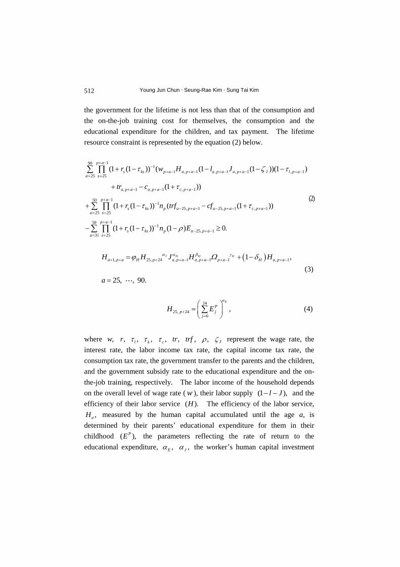
educational expenditure for the children, and tax payment. The lifetime
resource constraint is represented by the equation (2) below.
190
1
1 , 1 , 1 , 1 , 125 25
, 1 , 1 , 1
11
25, 1 25, 1 , 125
(1 (1 )) ( (1 (1 ))(1 )
(1 ))
(1 (1 )) ( (1 ))
p a
s ks p a a p a a p a a p a J l p aa s
a p a a p a c p a
p a
s ks p a p a a p a c p aa s
r w H l J
tr c
r n trf cf
50
25
1501
25, 131 25
(1 (1 )) (1 ) 0.p a
s ks p a p aa s
r n E
(2)
1, 25, 24 , 1 , 1 1 , 11 ,
25, , 90.
J H H H
a p a H p a p a a p a p a H a p aH H J H H
a
(3)
24
25, 246
,E
P
p jj
H E
(4)
where ,w ,r ,l ,k ,c ,tr ,trf , J represent the wage rate, the
interest rate, the labor income tax rate, the capital income tax rate, the
consumption tax rate, the government transfer to the parents and the children,
and the government subsidy rate to the educational expenditure and the on-
the-job training, respectively. The labor income of the household depends
on the overall level of wage rate ( w ), their labor supply (1 ),l J and the
efficiency of their labor service ( ).H The efficiency of the labor service,
,aH measured by the human capital accumulated until the age a, is
determined by their parents’ educational expenditure for them in their
childhood ( ),PE the parameters reflecting the rate of return to the
educational expenditure, ,E ,J the worker’s human capital investment
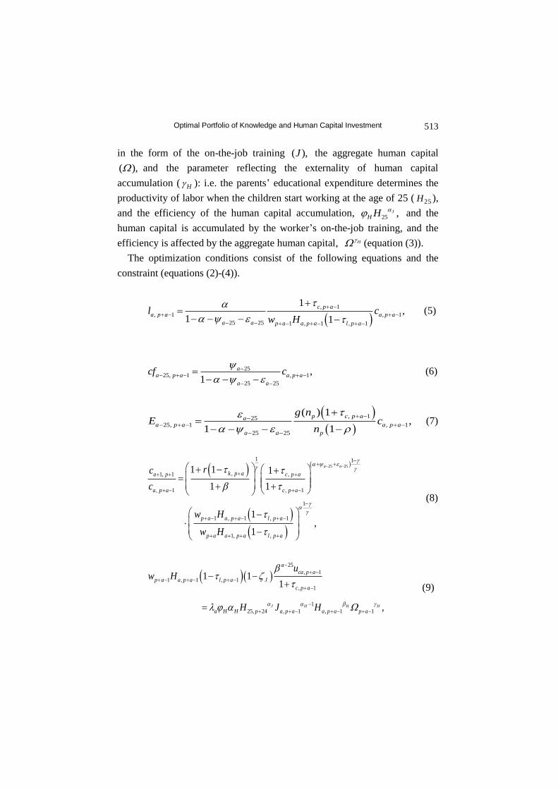
Optimal Portfolio of Knowledge and Human Capital Investment 513
in the form of the on-the-job training ( ),J the aggregate human capital
( ), and the parameter reflecting the externality of human capital
accumulation ( H ): i.e. the parents’ educational expenditure determines the
productivity of labor when the children start working at the age of 25 ( 25H ),
and the efficiency of the human capital accumulation, 25 ,J
H H and the
human capital is accumulated by the worker’s on-the-job training, and the
efficiency is affected by the aggregate human capital, H (equation (3)).
The optimization conditions consist of the following equations and the
constraint (equations (2)-(4)).
, 1
, 1 , 1
25 25 1 , 1 , 1
1,
1 1
c p a
a p a a p a
a a p a a p a l p a
l cw H
(5)
2525, 1 , 1
25 25
,1
aa p a a p a
a a
cf c
(6)
, 12525, 1 , 1
25 25
( ) 1,
1 1
p c p aaa p a a p a
a a p
g nE c
n
(7)
25 25
1 1
, 1, 1 ,
, 1 , 1
1
1 , 1 , 1
1, ,
1 1 1
1 1
1 ,
1
a a
k p aa p c p a
a p a c p a
p a a p a l p a
p a a p a l p a
rc
c
w H
w H
(8)
25
, 1
1 , 1 , 1
, 1
1
25, 24 , 1 , 1 1
1 11
,J H H H
a
ca p a
p a a p a l p a J
c p a
a H H p a p a a p a p a
uw H
H J H
(9)

Young Jun Chun Seung-Rae Kim Sung Tai Kim 514
25
, 1 25 25 , 1
(1 )
, 1
25 25 1 , 1 , 1
(1 )
25
25 25
(
, 125
25 25
1
1
1 1
1
( ) 1
1 1
a
ca p a a a a p a
c p a
a a p a a p a l p a
ap
a a
g n
p c p aa
a a p
u c
w H
n
g n
n
25) (1 )
.
a
(10)
1
1, 2 1 , 1
1 , 1 , 1 , 1 , 1 , 1
1
, 1 25, 24 , 1 , 1 1
1 1
1 1 1
1 Ω .J H H H
a p a p a k p a
p a a p a a p a a p a J l p a ca p a
a p a H H H p a p a a p a p a
r
w H l J u
H J H
(11)
The optimization conditions indicate the following features of the
household decision-making. The parents and children are altruistically
linked, and the resource allocation within the household is decided based on
the maximization of the weighted average of the parents’ welfare and the
children’s welfare. Therefore, given the total amount of the transfer income
for the household, the resource allocation is not affected by the distribution
of the transfer income from the government between the parents and the
children. The decrease in the number of the children increases the
educational expenditure per child, because we assume that ( )g n >0,
( )g n <0, while the magnitude of the consumption for each child is not
affected by the number of children. This reflects the fact that the parents
assign larger resource to the children’s education to improve the quality of
the children, when the constraint of the resource is mitigated by the decrease
in the number of children. The allocations of the parents’ consumption and
labor supply are the same as those in the standard life-cycle models. The

Optimal Portfolio of Knowledge and Human Capital Investment 515
on-the-job training hour is determined by its marginal cost,
1 1 ,a la JwH and its marginal benefit, 1
25 Ω .J H H H
a H H a a aH J H
The marginal cost of the on-the-job training is the after-tax wage rate less the
government subsidy per hour. The marginal benefit is the marginal effect
of the on-the-job training on the human capital, 1
25 Ω ,J H H H
H H a a aH J H
multiplied by the rate of return of the human capital increase, .a The rate
of return of the human capital investment consists of 2 components: the
human capital investment increases the wage income in the future; and it also
facilitates the human capital accumulation in the future.
2.2. Firms
The firms maximize their value ( ),V which is defined as the present
value of their profits, by choosing the input of the labor ( )L and the capital
( ),K the physical investment ( )I and the expenditure for the R&D ( ).Ry
The profit is the revenue minus the labor cost, the capital cost, the physical
investment, and the cost of R&D investment, 1 .Rsy The technology
of the firms is represented by the Cobb-Douglas production function of the
labor and the capital, with the labor-augmenting technological progress.
1
1 1 ,s
t j s s s s s s Rss t j t
V r Y w L r K I y
(12)
1 ,s s s sY K A L (13)
where , , , Y A
represent the output, the firm’s technology level, the
labor income share, and the government subsidy rate for the R&D. The
labor productivity is determined by the overall level of productivity of the
society, ,A and the human capital embodied in the individual’s labor
service, H (see equation (3)), which affects the labor input measured in
efficiency unit ( ).L
The evolutions of the physical capital and the technological level are

Young Jun Chun Seung-Rae Kim Sung Tai Kim 516
determined following equations (14) and (15).
1 1 ,s s K sK I K (14)
1 1 ,s s A s RsA A A y (15)
where K and A are the depreciation rates of physical capital and the
technology, and , , are the R&D technology parameters reflecting the
efficiency of R&D in new technology production, the contributions of the
existing technology and the contribution of the R&D investment to the new
technology production, respectively.
The firm’s maximization problem is represented by the following equation
(12).
11
1
1
1 1
1
1 ,
s
j s s s s s s s s Rss t j t
s s K s ss t
s A s Rs sss t
Z r K A L w L r K I y
I K K
A A y A
(16)
where and are the shadow values of the physical capital
accumulation equation and the technological evolution equation.
The optimization conditions consist of the equations (14), (15), and the
following equations (17)-(20).
11 ,s s s s sK A L A w
(17)
1 ,s s s s KK A L r (18)
1 11 1
11 1 0,s
j s s s s s s A s Rss t j
r K A L L A y
(19)

Optimal Portfolio of Knowledge and Human Capital Investment 517
1
11 1 .s
j s s Rss t j t
r A y
(20)
The equations (17)-(20) are the first order conditions for the labor input,
the capital input, the technological level, and the R&D investment.
Defining 1
1 ,s
s s jj
r
we get the following equation (19a).
1 11
1 1 1 1 1
1 1
1 1 1 1
1
1 1 .
s s s s s s
s s A s Rs
r K A L L
r A y
(19a)
The equation (17) shows the equalization of the marginal productivity of
labor and the wage rate, and the equation (18) that of the marginal
productivity of capital and the rental rate. The equation (19a) shows the
optimal condition of the evolution of the technological level. The present
value ( )s of the shadow value ,s which is the marginal value of
mitigating the constraint for technology level, can be interpreted as the
marginal return from the improvement of the technology. The marginal
return can be divided into 2 parts. The improvement of the technology
raises the production level in the future, represented by the first term of the
right hand side of the equation (19a), and it facilitates the technological
progress, represented by the second term.
The following equation (20a) is derived from the equation (20). The
equation (20a) shows the decision making process on the R&D investment.
11 .s s RsA y (20a)
The left hand side of (20a) represents the marginal cost of the R&D
investment. The effective marginal cost is the difference of the R&D
investment and the subsidy from the government. The right hand side is the
rate of return of the R&D investment, which is the multiplication of the term,

Young Jun Chun Seung-Rae Kim Sung Tai Kim 518
reflecting the effect of the R&D investment on the technological progress
1 ,s RsA y by the marginal return from the technological progress ( ).s
The equation (19a) indicates that the marginal return of the technological
progress is positively related with K and .L The decrease in the market
size resulting from the declining population, which reduces the labor input
and the capital accumulation, lowers the return of the technological progress
and the rate of return of the R&D investment, and reduces the R&D
investment. As a result, the technological progress will be delayed.
2.3. Government
The roles of government are the provision of the subsidy to the R&D
investment, the educational investment for the children and on-the-job
training, the provision of transfer payment to the households, and the
imposition of taxes to finance the expenditure. We assume that the
government maintains the balanced budget every period (see equation (21)).
24 90 24 90
., , , ,6 25 0 25
1
,
at at J t a t l t a t a t Rt at at at ata a a a
l t t k t t c t
E w H J y trf tr
w N rW C
(21)
90
25
1 ,t at at at ata
N H l J
(22)
90
25
,t at ata
W a
(23)
90 24
25 0
,t at at at ata a
C c cf
(24)
where , , , , a aa N W C represent the population and the asset-holding of
the aged a, the aggregate values of the labor supply, the asset-holdings, and
the consumption.
Optimal Portfolio of Knowledge and Human Capital Investment 519
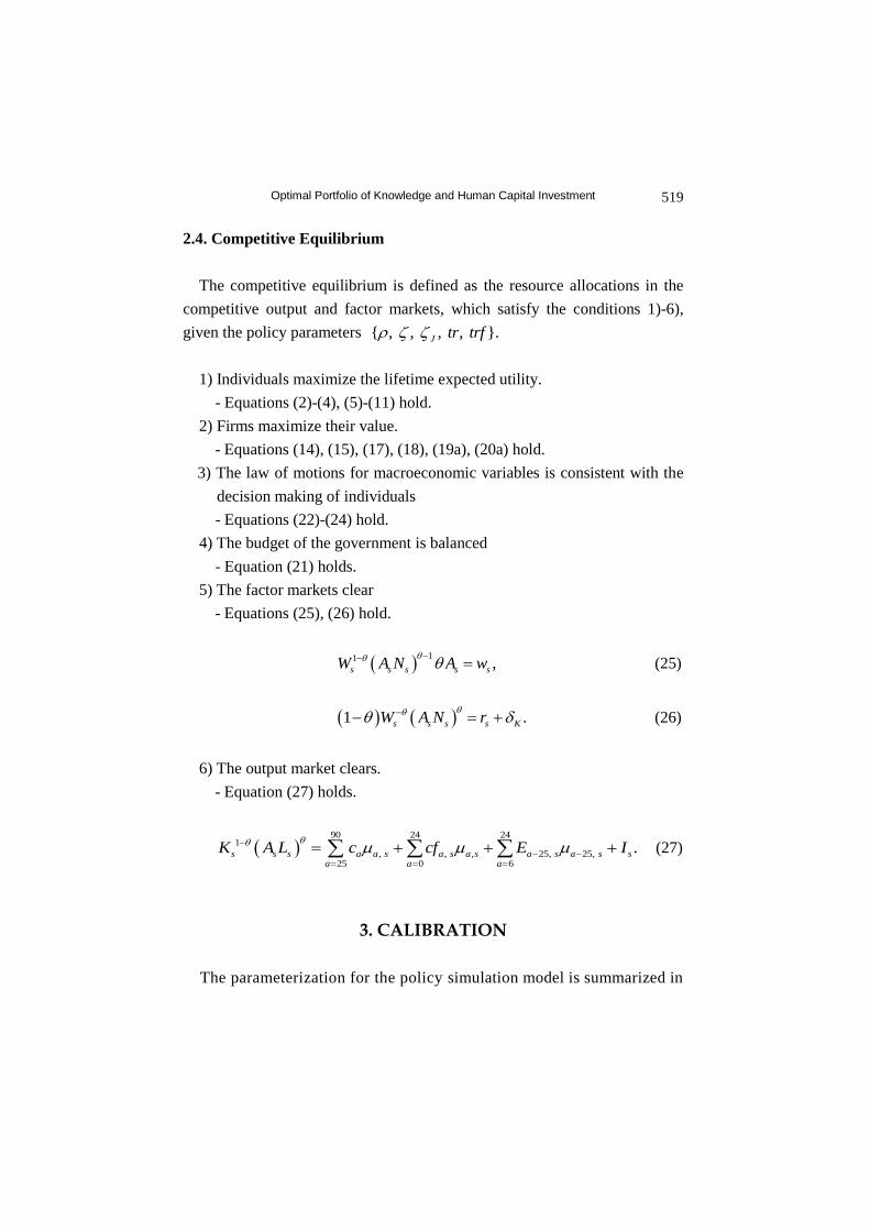
2.4. Competitive Equilibrium
The competitive equilibrium is defined as the resource allocations in the
competitive output and factor markets, which satisfy the conditions 1)-6),
given the policy parameters { , , , , }.J tr trf
1) Individuals maximize the lifetime expected utility.
- Equations (2)-(4), (5)-(11) hold.
2) Firms maximize their value.
- Equations (14), (15), (17), (18), (19a), (20a) hold.
3) The law of motions for macroeconomic variables is consistent with the
decision making of individuals
- Equations (22)-(24) hold.
4) The budget of the government is balanced
- Equation (21) holds.
5) The factor markets clear
- Equations (25), (26) hold.
11 ,s s s s sW A N A w
(25)
1 .s s s s KW A N r (26)
6) The output market clears.
- Equation (27) holds.
90 24 24
1
, , , 25, 25, 25 0 6
.s s s a a s a s a s a s a s sa a a
K A L c cf E I
(27)
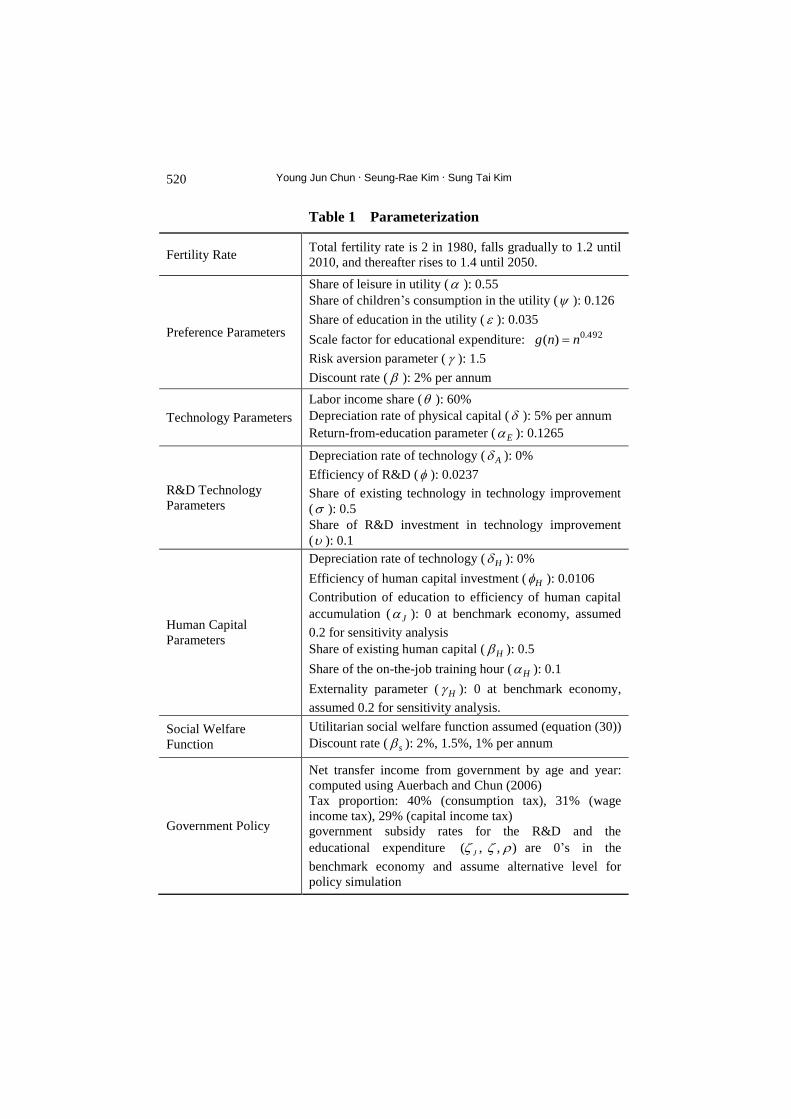
3. CALIBRATION
The parameterization for the policy simulation model is summarized in
Young Jun Chun Seung-Rae Kim Sung Tai Kim 520
Table 1 Parameterization
Fertility Rate Total fertility rate is 2 in 1980, falls gradually to 1.2 until
2010, and thereafter rises to 1.4 until 2050.
Preference Parameters
Share of leisure in utility ( ): 0.55
Share of children’s consumption in the utility ( ): 0.126
Share of education in the utility ( ): 0.035
Scale factor for educational expenditure: 492.0)( nng
Risk aversion parameter ( ): 1.5
Discount rate ( ): 2% per annum
Technology Parameters
Labor income share ( ): 60%
Depreciation rate of physical capital ( ): 5% per annum
Return-from-education parameter ( E ): 0.1265
R&D Technology
Parameters
Depreciation rate of technology ( A ): 0%
Efficiency of R&D ( ): 0.0237
Share of existing technology in technology improvement
( ): 0.5
Share of R&D investment in technology improvement
( ): 0.1
Human Capital
Parameters
Depreciation rate of technology ( H ): 0%
Efficiency of human capital investment ( H ): 0.0106
Contribution of education to efficiency of human capital
accumulation ( J ): 0 at benchmark economy, assumed
0.2 for sensitivity analysis
Share of existing human capital ( H ): 0.5
Share of the on-the-job training hour ( H ): 0.1
Externality parameter ( H ): 0 at benchmark economy,
assumed 0.2 for sensitivity analysis.
Social Welfare
Function
Utilitarian social welfare function assumed (equation (30))
Discount rate ( s ): 2%, 1.5%, 1% per annum
Government Policy
Net transfer income from government by age and year:
computed using Auerbach and Chun (2006)
Tax proportion: 40% (consumption tax), 31% (wage
income tax), 29% (capital income tax)
government subsidy rates for the R&D and the
educational expenditure ( , , )J are 0’s in the
benchmark economy and assume alternative level for
policy simulation

Optimal Portfolio of Knowledge and Human Capital Investment 521
table 1. We adopt the values for and , 1.5 and 0.02, to produce the
reasonable values for the aggregate wealth and the consumption profile.8)
We set 0.55 for , because the Ministry of Labor (2005) reported that the
proportion of labor hour out of the substitutable time is about 45%.9)
We
assume the parameters for shares of the children’s consumption and
educational expenditure as follows, reflecting that: (1) the proportion of the
expenditure for the children, including the consumption and the educational
expenditure, is estimated 35% of the baby boom generations in Korea (Son,
2011); and Kang and Hyun (2012) showed that the proportion of the
educational expenditure in the household consumption is 7%.
0.28 (1 ) 0.126, 0, , 24,
0, otherwisea
a
0.07 (1 ) 0.0315, 6, , 24.
0, otherwisea
a
The scale factor function of the educational expenditure is assumed 0.492( ) ,g n n based on the empirical findings of Lee (2008).
The demographic structure in the model is determined by the fertility rate,
because the model does not assume the mortality risk. We assume that the
total fertility rate has fallen from 2 (as of 1980) to the current level (1.2 as of
2010), and will rise to 1.4 until 2050, based on the projection of National
Statistics Office (2005).
The labor income share in the production function is assumed 60%, based
on the value reported in National Account. The depreciation rate of the
8) The previous empirical research showed a wide range of the estimate for the risk aversion
parameter , and there is scant evidence of the appropriate value for . For the
extensive literature survey on the parameter estimates, see Auerbach and Kotlikoff (1987a). 9)
According to the Ministry of Labor (2005), the average labor hour per week of the
representative worker is 45 hours. Assuming that the time per week under the individual
discretion, excluding the time for sleeping, eating, and commuting, is about 97 hours, the
proportion of the labor is about 48%.

Young Jun Chun Seung-Rae Kim Sung Tai Kim 522
physical capital is assumed 5% per annum, based on its estimated value
reported in Pyo (2003).
We set 0% for the depreciation rate of the technology, following Jones
(1995). We choose the values for the parameters reflecting the contribution
of the existing technology and the R&D investment in technology production
function using the equation (15). The equation (15) can be rewritten as the
following equation (15a).
11 .s ss Rs
s
A AA y
A
(15a)
On the balanced growth path, the left hand side of the equation (15a) is
constant. Taking the natural log function and taking derivatives both sides
of the equation, we get the equation (28), which shows the long-run
relationship between and .
/.
/ 1R R
A A
y y
(28)
The left hand side of the equation (28) is the elasticity of productivity
growth with respect to R&D investment. Lee et al. (2010) reported its
estimated value around 0.2 for several OECD countries.10)
We cannot solve
for both and using the estimated value using the equation (28) only.
We choose 0.1 and 0.5 for the value of and in the benchmark
economy and assume different combination for the sensitivity analysis,11)
and
choose 0.0237 for the values of in order to reproduce the average
productivity growth for the period 2000-2005, which was estimated by
Kwack (2007).12)
10) Lee et al. (2010) also reported the estimated elasticity for several OECD countries: 0.220
(for US), 0.288 (Japan), 0.116 (Canada), 0.147 (Italy), and 0.182 (Korea). 11) We try the sensitivity analysis assuming alternative values satisfying equation (28):
( , ) =(0.25, 0.15) or (0.75, 0.05). 12) Kwack (2007) reported that the productivity growth due to the total factor productivity is

Optimal Portfolio of Knowledge and Human Capital Investment 523
Figure 1 Transfer Income from Government ([1])
We choose 0.1265 for ,E based on the estimate for the elasticity of
income of the children with respect to the educational expenditure by An and
Jeon (2008). We assume that the human capital accumulation function is
the same as that of technology production through the R&D,
, ,H H except for (0.0106),H so that we can produce a
reasonable value for the time devoted to the on-the-job training. We set 0’s
for the parameters for the contribution of the education to the efficiency of
human capital accumulation, ,J and the externality of the aggregate
human capital, ,H at benchmark economy and assume the alternative
values for the sensitivity analysis. We also assume that 0,H following
Hechman and Taber (1998).
We assume the government subsidy rates for the R&D and the educational
expenditure ( , , )J are 0’s in the benchmark economy, and investigate
the effect of the government subsidy by assuming alternative levels. We
compute the transfer income from the government by age and year, shown in
1.48% and 0.82% due to the human capital accumulation for the period 2000-2005. We
choose the value of that reproduces 2.30% for the labor productivity for that period.

Young Jun Chun Seung-Rae Kim Sung Tai Kim 524
figure 1, using the method of Auerbach and Chun (2006).13)
The proportion
of the tax revenue by the tax base is assumed 40% (consumption tax), 31%
(wage income tax), 29% (capital income tax) based on the records in recent
years.
4. FINDINGS
We simulate 4 economies. The economy [1] is our benchmark economy
where the government does not provide the subsidy for the R&D investment,
that for the educational expenditure, or that for the on-the-job training. In
this economy, we assume the fertility rate estimates by the NSO (2005) and
reflect the current public transfer program.14)
The economy [2] simulates
the provision of the subsidy to the R&D of the firms, the economy [3] that to
the educational expenditure of the households, and the economy [4] that to
the on-the-job training of the workers. In all three economies, we assume
that the subsidy rate is 40% ( 0.4).J
4.1. Benchmark Economy
The resource allocations in our benchmark economy ([1]) are summarized
in table 2 and figure 2. As of the year 2000 of the benchmark economy, the
capital-output ratio is 3.65, the average of workers’ share of the labor hour
out of total substitutable time is 34.9%, and the savings rate is 19.4%. Even
though the share of the labor hour is lower than that reported in the Ministry
of Labor (2005) (0.48), which surveyed on the labor conditions of the regular
workers, the value is a reasonable compromise, considering the existence of
13) In order to incorporate the generational accounts into our general equilibrium model, we
adjusted the absolute level of the public transfers for each age in each year considering the
overall change in the wage level. 14)
Under the current public transfer programs, the government transfer expenditure is
projected to increase up to 22% of GDP until around 2060, due to the maturing of the
social welfare system including the National Pension and the Public Long-Term Care
Insurance, and the population aging.

Optimal Portfolio of Knowledge and Human Capital Investment 525
Table 2 Resource Allocation (for the year 2000)
Capital-Output Ratio
Labor Hour (worker)
Ratio of OJT Hour to Labor Hour (%)
Savings Rate (%)
Ratio of Consumption (except for educational exp) to GDP (%)
Ratio of Educational Expenditure to GDP (%)
Ratio of Educational Expenditure to Household Consumption
(for households with children %)
Ratio of Educational Expenditure to Household Consumption
(for the whole household, %)
R&D Investment / GDP (%)
3.65
0.349
1.5
19.4
79.3
1.1
4.8
1.4
2.3
the daily workers, the temporary workers, and other non-regular workers,
whose labor hour is much shorter than the regular workers, and their large
proportion in the labor force in Korea. The low level of the net savings rate
generated, 1.15% (=19.4%–3.65(K/GDP)×5%), well reflects the low rate of
the savings rates and their downward trend of the recent years.
The educational expenditure computed in the model is 1.1% of GDP, 1.4%
of the consumption of the whole household, 4.8% of the consumption of the
household with children, 6.3% of the consumption of the household with the
children aged 6-24, which is close to the estimate by Kang and Hyun (2008),
7% of household consumption with children. The ratio of the R&D to GDP
in the initial year computed is 2.3%, which is close to its actual magnitude of
the recent years (2.3%, OECD (2011)). The ratio of the time devoted to the
on-the-job training to the labor hour is 1.5%, which is close to the estimate
by the Kim et al. (2011). They showed that the average time devoted to the
job training by the wage workers, who have participated into the job training,
is 37 hours a year. This is about 1.5% of the annual working hour, taking
into account: the average labor hour per week of the regular workers is 48
hours (the Ministry of Labor, 2005); and a year is about 52 weeks.

Young Jun Chun Seung-Rae Kim Sung Tai Kim 526
Figure 2 Base Case Economy
0
20
40
60
80
100
120
140
160
2010 2030 2050 2070 2090 2110 2130 2150 2170
year
GDP
0
1
2
3
4
5
6
7
8
9
10
2010 2030 2050 2070 2090 2110 2130 2150 2170
year
GDP per capita
0
100
200
300
400
500
600
2010 2030 2050 2070 2090 2110 2130 2150 2170
year
capital
0
5
10
15
20
25
30
35
2010 2030 2050 2070 2090 2110 2130 2150 2170
year
Labor supply
0
0.005
0.01
0.015
0.02
0.025
2010 2030 2050 2070 2090 2110 2130 2150 2170
year
OJT/Labor hour
0
0.01
0.02
0.03
0.04
0.05
0.06
0.07
0.08
0.09
2010 2030 2050 2070 2090 2110 2130 2150 2170
year
Educational Exp. per child
0
0.5
1
1.5
2
2.5
2010 2030 2050 2070 2090 2110 2130 2150 2170
year
R&D
0
100
200
300
400
500
600
700
2010 2030 2050 2070 2090 2110 2130 2150 2170
year
Return from R&D
0
2
4
6
8
10
12
14
2010 2030 2050 2070 2090 2110 2130 2150 2170
year
Firm Technology
0
0.002
0.004
0.006
0.008
0.01
0.012
0.014
0.016
0.018
0.02
2010 2030 2050 2070 2090 2110 2130 2150 2170
year
Growth Rate of Firm Technology
0
0.05
0.1
0.15
0.2
0.25
2010 2030 2050 2070 2090 2110 2130 2150 2170
year
Gov. Exp / GDP
0
5
10
15
20
25
30
2010 2040 2070 2100 2130 2160
year
Tax Rates
labor income
capital income
consumption
0
0.5
1
1.5
2
2.5
3
3.5
4
1915 1935 1955 1975 1995 2015 2035 2055 2075 2095
year of birth
Welfare 1
0
0.5
1
1.5
2
2.5
3
3.5
4
1915 1935 1955 1975 1995 2015 2035 2055 2075 2095
year of birth
Welfare 2

Optimal Portfolio of Knowledge and Human Capital Investment 527
The resource allocations after the initial period are reported figure 2. The
GDP is projected to increase until 2040s, and to decrease thereafter because
of the decrease in the capital stock and the labor supply due to the population
aging. However, the GDP per capita will continue to increase because of the
technological progress. The technological progress results from the
educational expenditure, the on-the-job training, and the R&D investment.
The educational expenditure is projected to increase because of the decrease
in the number of the children per parent, due to the low fertility rate. The
increase in the educational expenditure will improve the labor productivity
and the marginal benefit of the OJT, (equations (4), (9)), which will increase
the time devoted to the OJT. The R&D investment is projected to gradually
decrease, because of the decrease in the return from the R&D. The decrease
in the return from the R&D is due to the decrease in the market size and the
production level (see equation (19a)), resulting from the population decrease.
The aggregate human capital is projected to rise up to the level 1.65 times as
high as that at the initial period, while the firm’s technology to rise up to the
level 11.3 times as high as that at the initial period. These results indicate
that the future labor productivity will be more dependent upon the R&D
investment than on the human capital investment, because the population
decrease in the future will restrict the growth of the aggregate human capital.
The model produces the annual rate of the firm’s technological progress for
the recent 10 (30) years is 2.0% (2.2%), which belongs to the range of the
estimates of the total factor productivity by the previous empirical studies.15)
To compute the welfare across generations, we use the following equation
(29). We solve for ,px the proportional change in the adult consumption,
the leisure, the children's consumption, and the educational expenditure of
the generation born in the initial year (p=0, i.e. the year 1980), required to
equalize the lifetime expected utility of each generation to that of the cohort
born in the initial year.
15) These studies include Pilat (1995), Young (1995), Kwack (1997), and Yoon and Lee (1998).
The estimates for the total factor productivity growth rate belong to the range 2-4% per
annum.

Young Jun Chun Seung-Rae Kim Sung Tai Kim 528
2590
( )
, -1 , -1 25, 1 25, 125
2590 ( )
,0 1 ,0 -1 0 25,0 1 25,0 125
1, , ,
1
1, , , .
1
p
p
a
g n
a p a a p a p a p a a p aa
ag n
a a p a a p a a p a a pa
u c l n cf E
u c x l x n cf x E x
(29)
The labor productivity growth will improve the welfare of the future
generations. The welfare level of the future generations born in 2100 is 3.4
times as high as the level of the welfare of the current generations, and the
welfare level for the cohorts born after 2100 will rise continuously because of
continuous growth.
4.2. Policy Simulations
The provision of the subsidy to the R&D investment is shown to improve
the GDP per capita and the welfare of the future generations more than that
to the educational expenditure or to the on-the-job training. The provision
of the subsidy which covers the 40% of the R&D investment cost will
improve the GDP per capita by up to 6%, while that which covers the same
proportion of the educational expenditure will not raise the GDP per capita.
Moreover, the provision of the subsidy to the OJT will lower the GDP level,
even though the magnitude of the GDP reduction is small.16)
The
differential effect of these 3 subsidy schemes, despite almost the same impact
on the R&D investment, the educational expenditure, and the time devoted to
the job training, is due to difference in the effect on the capital accumulation
and the labor supply. The subsidy to the educational expenditure will
reduce the savings and the wealth accumulation because of the increase in the
educational expenditure by up to 80%, even though it will raise the labor
productivity by 6% in the long run. The subsidy to the job training will
16) The figure 3 shows that the provision of the subsidy to the on-the-job training lowers the
GDP per capita for some period after its introduction. It is because its provision increases
the time allocated to the on-the-job training and decreases the labor hour. The human
capital accumulation through the on-the-job training is shown to offset the loss of
production due to the decrease in the labor hour in the long run.
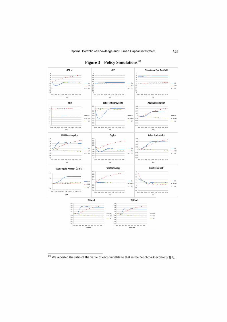
Optimal Portfolio of Knowledge and Human Capital Investment 529
Figure 3 Policy Simulations17)
0.88
0.9
0.92
0.94
0.96
0.98
1
1.02
1.04
1.06
1.08
2010 2030 2050 2070 2090 2110 2130 2150 2170
year
GDP pc
Edu
R&D
OJT
0
0.2
0.4
0.6
0.8
1
1.2
1.4
1.6
1.8
2
2010 2030 2050 2070 2090 2110 2130 2150 2170
year
OJT
Edu
R&D
OJT
0
0.2
0.4
0.6
0.8
1
1.2
1.4
1.6
1.8
2
2010 2030 2050 2070 2090 2110 2130 2150 2170
year
Educational Exp. Per Child
Edu
R&D
OJT
0
0.2
0.4
0.6
0.8
1
1.2
1.4
1.6
1.8
2
2010 2030 2050 2070 2090 2110 2130 2150 2170
year
R&D
Edu
R&D
OJT
0.93
0.94
0.95
0.96
0.97
0.98
0.99
1
1.01
2010 2030 2050 2070 2090 2110 2130 2150 2170
year
Labor (efficiency unit)
Edu
R&D
OJT
0.92
0.94
0.96
0.98
1
1.02
1.04
1.06
1.08
2010 2030 2050 2070 2090 2110 2130 2150 2170
year
Adult Consumption
Edu
R&D
OJT
0.92
0.94
0.96
0.98
1
1.02
1.04
1.06
1.08
2010 2030 2050 2070 2090 2110 2130 2150 2170
year
Child Consumption
Edu
R&D
OJT
0.9
0.92
0.94
0.96
0.98
1
1.02
1.04
1.06
1.08
2010 2030 2050 2070 2090 2110 2130 2150 2170
year
Capital
Edu
R&D
OJT
0.94
0.96
0.98
1
1.02
1.04
1.06
1.08
2010 2030 2050 2070 2090 2110 2130 2150 2170
year
Labor Productivity
Edu
R&D
OJT
0.94
0.96
0.98
1
1.02
1.04
1.06
1.08
2010 2030 2050 2070 2090 2110 2130 2150 2170
year
Firm Technology
Edu
R&D
OJT
0.8
0.9
1
1.1
1.2
1.3
1.4
1.5
2010 2030 2050 2070 2090 2110 2130 2150 2170
year
Gov't Exp / GDP
Edu
R&D
OJT
0.95
0.96
0.97
0.98
0.99
1
1.01
1.02
1.03
1.04
1.05
1915 1935 1955 1975 1995 2015 2035 2055 2075 2095
birth year
Wefare 1
Edu
R&D
OJT
0.95
0.96
0.97
0.98
0.99
1
1.01
1.02
1.03
1.04
1.05
1915 1935 1955 1975 1995 2015 2035 2055 2075 2095
year of birth
Welfare 2
Edu
R&D
OJT
17) We reported the ratio of the value of each variable to that in the benchmark economy ([1]).

Young Jun Chun Seung-Rae Kim Sung Tai Kim 530
reduce the savings, the wealth accumulation, and the labor supply due to the
increase in the time for the job training, even though it will raise the
aggregate human capital by 1%. Moreover, the subsidy has little impact on
the labor productivity, because the decrease in the capital accumulation
resulting from the provision of the subsidy will lower the productivity of the
labor. On the other hand, the subsidy to the R&D is projected to improve
the firm’s technology by up to 6%, without negative impacts on the wealth
accumulation or the labor supply.18)
Another important factor affecting the improvement of the firm’s
technology and the human capital investment and the economic growth is the
increase in the tax burden. The ratio of the government expenditure to GDP
increases most in the case of the subsidy to the R&D in the first year of the
policy implementation, followed by that to the educational expenditure and
that to the on-the-job training. In future periods, the ratio increases most in
the case of the subsidy to the educational expenditure, followed by that to the
on-the-job training and that to the R&D. The ratio is lowest in the future in
the case of the subsidy to the R&D, due to the fact that it raises the GDP
most. The proportional increase in the tax burden will decrease overtime,
because the tax burden has a rising trend in the benchmark economy. In the
future period, the difference in the proportional increase in the tax burden is
not large, while they have differential effect on the efficiency of labor, which
indicates the differential effects of these policies on the welfare of the future
generations.
The effects on the welfare of the three policies are quite different. The
implementation of the education subsidy improves the welfare of the cohorts
18)
The differential effects of the subsidies to the R&D, the educational expenditure, and the
OJT, are consistent with the findings of the previous empirical researches: the R&D
investment and the human capital investment contributed significantly to the economic
growth, while the job training programs did not have significant effects on the job finding
rate or the wage level. Acevedo (2008) presented that the private and public R&D stocks
accounted for 16% and 19% of the economic growth respectively during the period 1976-
2009. Kim (2011) showed that the human capital accumulation accounted for 1.3%p of
the economic growth rate during the period 1980-2004. Lee (2005) showed that the job
training programs did not raise the job finding rate or the wage level when the workers are
reemployed after the job training.

Optimal Portfolio of Knowledge and Human Capital Investment 531
who will be born relatively early, while that of the R&D subsidy the welfare
of those who will be born in later years, because the productivity
improvement is realized earlier in the case of the former than in the case of
the latter policy implementation. In the case of the subsidy to the on-the-job-
training does not improve the welfare because of the limited improvement of
the labor productivity, the decrease in the GDP per capita and the
consumptions, and the increase in tax burden.
Despite its little impact on the GDP per capita, the subsidy to the
education improve the overall level of the welfare because it raises the labor
productivity, increases the consumption for the adults and the children. We
report two measures of the welfare effect: one taking into account the “joy of
giving,” the increase in the utility due to the increase in the educational
expenditure for the children (“welfare 1”); and one without consideration of
the joy of giving (“welfare 2”). Comparison of the two measures shows
that about 30% of the welfare improvement due to the education subsidy is
accounted for by the increase in the joy of giving.
4.3. Optimal Combination of the Subsidies
In this section, we search for the optimal combination of the three
subsidies. We have shown the differential effects of the subsidies to the
R&D, the educational investment, and the on-the-job training on the
improvement of the productivity, and tax burden across generations.
Despite the differential impacts on productivity, all three subsidy schemes
improve the productivity. However, the subsidy schemes may cause the
intergenerational redistribution. The provision of the subsidy to the R&D
investment will improve the welfare of the future generations, who are alive
in the periods when the improvement of the productivity due to the subsidy is
realized. Because of the time lag between the provision of the subsidy and
the realization of the efficiency gain, and the increase in the tax burden to
finance the subsidy program, the current generations’ welfare improvement
may be very limited. The optimal level of the subsidy rates is also an
Young Jun Chun Seung-Rae Kim Sung Tai Kim 532
important issue, because there is a trade-off regarding its level. The
increase in the subsidy rate improves the productivity in larger scale, while it
causes larger increase in the tax rates.
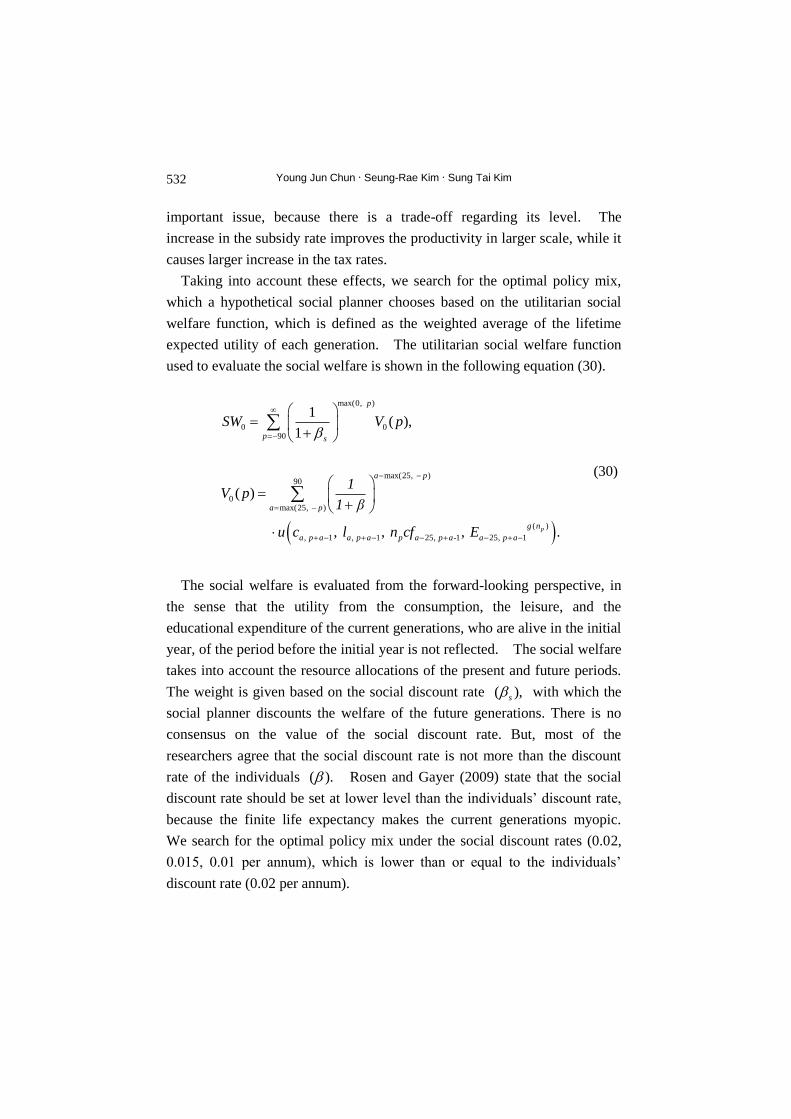
Taking into account these effects, we search for the optimal policy mix,
which a hypothetical social planner chooses based on the utilitarian social
welfare function, which is defined as the weighted average of the lifetime
expected utility of each generation. The utilitarian social welfare function
used to evaluate the social welfare is shown in the following equation (30).
max(0, )
0 090
max(25, )90
0max(25, )
( )
, 1 , 1 25, -1 25, 1
1( ),
1
( )
, , , .p
p
p s
a p
a p
g n
a p a a p a p a p a a p a
SW V p
1V p
1 β
u c l n cf E
(30)
The social welfare is evaluated from the forward-looking perspective, in
the sense that the utility from the consumption, the leisure, and the
educational expenditure of the current generations, who are alive in the initial
year, of the period before the initial year is not reflected. The social welfare
takes into account the resource allocations of the present and future periods.
The weight is given based on the social discount rate ( ),s with which the
social planner discounts the welfare of the future generations. There is no
consensus on the value of the social discount rate. But, most of the
researchers agree that the social discount rate is not more than the discount
rate of the individuals ( ). Rosen and Gayer (2009) state that the social
discount rate should be set at lower level than the individuals’ discount rate,
because the finite life expectancy makes the current generations myopic.
We search for the optimal policy mix under the social discount rates (0.02,
0.015, 0.01 per annum), which is lower than or equal to the individuals’
discount rate (0.02 per annum).

Optimal Portfolio of Knowledge and Human Capital Investment 533
Table 3 Optimal Combination of Subsidy Rates (%)
( , ,J )
=0.51)
=0.11)
J =0.01)
H =0.01)
<1>
=0.25
=0.15
J =0.0
H =0.0
<2>
=0.75
=0.05
J =0.0
H =0.0
<3>
=0.5
=0.1
J =0.2
H =0.0
<4>
=0.5
=0.1
J =0.0
H =0.2
<5>
=0.5
=0.1
J =0.2
H =0.2
Based on Welfare 12)
s =0.020 (0, 50, 75) (0, 50, 75) (0, 55, 80) (0, 50, 80) (0, 50, 80) (0, 50, 80)
s =0.015 (0, 60, 80) (0, 55, 80) (0, 60, 80) (0, 60, 80) (0, 60, 80) (0, 60, 80)
s =0.010 (0, 65, 80) (0, 60, 80) (0, 70, 80) (0, 70, 80) (0, 60, 80) (0, 70, 80)
Based on Welfare 23)
s =0.020 (0, 50, 65) (0, 45, 65) (0, 55, 70) (0, 50, 70) (0, 50, 70) (0, 50, 70)
s =0.015 (0, 55, 70) (0, 55, 70) (0, 60, 70) (0, 60, 70) (0, 60, 70) (0, 60, 70)
s =0.010 (0, 65, 75) (0, 60, 70) (0, 65, 75) (0, 60, 70) (0, 60, 70) (0, 70, 80)
Notes: 1) Benchmark case. 2) Welfare 1 takes account of the welfare from the “job of
giving”. 3) Welfare 2 disregards the welfare from the “job of giving”.
The numbers in table 3 are the optimal subsidy rates to the job training, the
R&D, and the education. The optimal policy combination under the
assumption of 2% social discount rate consists of: 50% subsidy to the R&D
investment, 75% subsidy to the educational investment, and 0% subsidy to
the on-the-job training.19)
The welfare gain of the subsidies to the R&D and
the educational investment is quite large. Figure 4 shows that the welfare
gain under the optimal combination of the subsidies at the benchmark case is
about 1.2% of the welfare at the base-case economy without any subsidy.
Assuming lower discount rates raises the optimal subsidy rate to the R&D
investment up to 65% and the optimal subsidy rate to the educational
investment up to 80%. Using the welfare 2 as the welfare measure lowers
the optimal subsidy rate to the education a little to 65-75%.
19)
The optimal subsidy rate to the OJT is 0, because the provision of the subsidy to the OJT
does not improve the welfare, as shown in section 4.2.

Young Jun Chun Seung-Rae Kim Sung Tai Kim 534
Figure 4 Welfare Gain (% of Welfare Benchmark)
4.4. Sensitivity Analysis
We try the sensitivity analyses assuming alternative values of parameters,
, , , .J H We compute 5 additional economies assuming: <1>
( , ) (0.25, 0.15); <2> ( , ) (0.75, 0.05); <3> ( , , )J
(0.5, 0.1, 0.2); <4> ( , , ) (0.5, 0.1, 0.2);H and <5> ( , , , )J H
(0.5, 0.1, 0.2, 0.2). Assumptions <1> and <2> are for the sensitivity
analysis for the variation of , , which produces the same elasticity of the
firm’s technological progress with respect to the R&D investment as that in
the benchmark economy where ( , ) (0.5, 0.1). Assumptions <3>,
<4>, <5> are to check the sensitivity of the results due to the change in the
human capital accumulation process: <3> assumes the existence of the
contribution of the education to the efficiency of the human capital
accumulation; <4> assumes the existence of the externality of the aggregate
human capital; and <5> assumes both the factors.
Figure 5 shows that the alternative assumptions on the firm’s technological
process and the human capital accumulation process do not produce the
qualitatively different results. The subsidy to the R&D is more effective to
raise the GDP per capita than that to the education, and that to the job training
0
0.3
0.5
0.65
0.8
-1.25
-0.75
-0.25
0.25
0.75
1.25
0
0.1
0.2
0.3
0.4
0.45 0.5
0.55 0.6
0.65 0.7
0.75 0.8
0.85
0.9
Subsidy rateto R&D
Subsidy rate to Education
Figure 4. Welfare Gain (% of welfare at benchmark)

Optimal Portfolio of Knowledge and Human Capital Investment 535
Figure 5 Sensitivity Analysis20)
[GDP per Capita]
0.9
0.95
1
1.05
1.1
2010 2030 2050 2070 2090 2110 2130 2150 2170
year
<1>
Edu
R&D
OJT
0.9
0.92
0.94
0.96
0.98
1
1.02
1.04
1.06
2010 2030 2050 2070 2090 2110 2130 2150 2170
year
<2>
Edu
R&D
OJT
0.88
0.9
0.92
0.94
0.96
0.98
1
1.02
1.04
1.06
1.08
2010 2030 2050 2070 2090 2110 2130 2150 2170
year
<3>
Edu
R&D
OJT
0.88
0.9
0.92
0.94
0.96
0.98
1
1.02
1.04
1.06
1.08
2010 2030 2050 2070 2090 2110 2130 2150 2170
year
<4>
Edu
R&D
OJT
0.88
0.9
0.92
0.94
0.96
0.98
1
1.02
1.04
1.06
1.08
2010 2030 2050 2070 2090 2110 2130 2150 2170
year
<5>
Edu
R&D
OJT
[Welfare 1]
0.95
0.96
0.97
0.98
0.99
1
1.01
1.02
1.03
1.04
1.05
1915 1935 1955 1975 1995 2015 2035 2055 2075 2095
birth year
<1>
Edu
R&D
OJT
0.95
0.96
0.97
0.98
0.99
1
1.01
1.02
1.03
1.04
1915 1935 1955 1975 1995 2015 2035 2055 2075 2095
birth year
<2>
Edu
R&D
OJT
0.94
0.96
0.98
1
1.02
1.04
1.06
1915 1935 1955 1975 1995 2015 2035 2055 2075 2095
birth year
<3>
Edu
R&D
OJT
0.95
0.96
0.97
0.98
0.99
1
1.01
1.02
1.03
1.04
1.05
1915 1935 1955 1975 1995 2015 2035 2055 2075 2095
birth year
<4>
Edu
R&D
OJT
0.92
0.94
0.96
0.98
1
1.02
1.04
1.06
1915 1935 1955 1975 1995 2015 2035 2055 2075 2095
birth year
<5>
Edu
R&D
OJT
Notes: <1>: ( , )=(0.25, 0.15) <2>: ( , )=(0.75, 0.05); <3>: ( , , J ) =(0.5,
0.1, 0.2); <4>: ( , , H )=(0.5, 0.1, 0.2); <5>: ( , , J , H )=(0.5, 0.1, 0.2,
0.2).
20)
We reported the ratio of the value of each variable to that in the benchmark economy.

Young Jun Chun Seung-Rae Kim Sung Tai Kim 536
is not effective to raise GDP per capita. The subsidies to the R&D and the
education improve the welfare of the future generations, while that to the job
training does not improve the welfare, because of the decrease in the labor
supply, the resulting decrease in the labor income and the wealth
accumulation. Table 3 also shows that the alternative assumption on the
parameters does not change the optimal combination of the subsidy rates to
the R&D, the education, and the job training much.
The results of the sensitivity analysis indicate the potential importance of
the role of education in improving efficiency of the human capital
accumulation through the job training and the externality of the human
capital accumulation. In the economies <3> and <5>, the effects of the
subsidy to the education on the GDP per capita level are amplified by
incorporating the roles, i.e. by assuming positive numbers for , .J H
There is little empirical findings regarding the values for , J H for Korea.
However, it is not likely that J and H are as high as 0.2, because the
estimates for these parameters for other countries, are not so high.21)
5. CONCLUSION
We have searched for the optimal combination of the firm’s technology
and human capital accumulation through the education and the job training,
using a general equilibrium model. The characteristic of the non-rivalry of
the technology and human capital induces the private agents’ decision-
making, which causes the inefficient resource allocation: i.e. they do not take
into account the spillover effects of the improvement of the firm’s
technology over the efficiency of the human capital investment, and vice
versa. More importantly, the finite-horizon economic agents do not fully
take account of the externality of the improvement of the technology and the
21)
For example, Ciccone and Peri (2006) showed a very low value of the education
externality: the point estimates of the external return to a 1-year increase in average
schooling are around 0 at the city level and around 2% at the state level in US, which
indicates 0 or 0.02 for .H
Optimal Portfolio of Knowledge and Human Capital Investment 537
human capital accumulation. Therefore, the optimal portfolio of the
knowledge investment in the form of the R&D investment and the human
capital investment in the form of the educational investment and the job
training should be attained by the optimal subsidy combination, which
enables the internalization of the benefits of the spillover effects of the
improvement of the firm’s knowledge (or the worker’s knowledge).
The policy simulations, using a general equilibrium model, which
incorporates these aspects of the knowledge investment and human capital
investment, the characteristics of the Korean economy and the knowledge
production and the human capital investment process, show that: (1) the
subsidy to the R&D investment is more effective to improve the productivity
and the welfare of the future generations than that to the educational
investment (or to the job training); (2) compared with the difference in the
impact of the subsidy schemes on the productivity, the difference in the
increase in the tax burden due to the provision of the subsidy is smaller,
which indicates the differential effects on the welfare; and (3) the optimal
combination of the subsidy schemes, taking into account differential impact
on the productivity, the tax burden, and the welfare across generations, is
shown to be 50-65% subsidy to the R&D investment, 65-80% subsidy to the
educational investment, and no subsidy to the job training.
REFERENCES
Acevedo, Sebastian, “Measuring the Impact of Human Capital on the
Economic Growth of South Korea,” The Journal of Korean Economy,
9(1), 2008, pp. 113-139.
Aghion, Phillippe and Peter Howitt, “A Model of Growth through Creative
Destruction,” Econometrica, 60(2), March 1992, pp. 323-351.
Altig, David, Alan J. Auerbach, Laurence J. Kotlikoff, Kent A. Smetters, and
Jan Walliser, “Simulating Fundamental Tax Reform in the United
States,” American Economic Review, 91(3), June 2001, pp. 574-595.

Young Jun Chun Seung-Rae Kim Sung Tai Kim 538
An, Chong-Bum and Seung Hoon Jeon, “Intergenerational Transfer of
Educational Achievement and Household Income,” Korean Journal
of Public Finance, 1(1), 2008, pp. 119-142 (in Korean).
Arrow, Kenneth J., “Economic Welfare and the Allocation of Resources for
Inventions,” in R. R. Nelson, ed., The Rate and Direction of Inventive
Activity, Princeton, NJ: Princeton University Press for the NBER,
1962.
Auerbach, Alan J. and Laurence Kotlikoff, “Simulation Mothodology,”
Chapter 4 of Dynamic Fiscal Policy, Cambridge University Press,
1987a.
____________, “Effect of a Demographic Transition and Social Security’s
Policy Response,” Chapter 11 of Dynamic Fiscal Policy, Cambridge
University Press, 1987b.
____________, “Social Security,” Chapter 10 of Dynamic Fiscal Policy,
Cambridge University Press, 1987c.
Auerbach, Alan J. and Young Jun Chun, “Generational Accounting in
Korea,” Journal of Japanese and International Economies, 20(2),
June 2006, pp. 234-268.
Bank of Korea, National Account, Each year.
Becker, Gary, “On the Interaction between the Quantity and the Quality of
Children,” Journal of Political Economy, 81(2), 1973, pp. S279-S288.
Becker, Gary, Kevin Murphy, and Robert Tamura, “Human Capital, Fertility,
and Economic Growth,” Journal of Political Economy, 98(5), Part 2,
1990, pp. S12-S37.
Bloom, David E., David Canning, and Grunther Fink, “Implications of
Population Aging for Economic Growth,” NBER Working Paper, No.
16705, 2011.
Chun, Young Jun, “Population Aging, Fiscal Policies, and National Saving:
Prediction for Korean Economy,” in Takatoshi Ito and Andrew Rose,
eds., Fiscal Policy and Management in East Asia, NBER East Asia
Seminar on Economics Volume 16, University of Chicago Press and
NBER, 2007.

Optimal Portfolio of Knowledge and Human Capital Investment 539
____________, “Green Growth Strategy and Economic Growth,” Korean
Journal of Applied Economics, 13(1), 2011, pp. 135-174 (in Korean).
____________, “The Growth Effects of Population Aging in an Economy
with Endogenous Technological Progress,” Unpublished Research
Paper, 2012.
Ciccone, Antonio and Giovanni Peri, “Indentifying Human-Capital
Externalities: Theory with Applications,” Review of Economic
Studies, 73(2), 2006, pp. 381-412.
Grossman, Gene and Elhanan Helpman, Innovation and Growth in the
Global Economy, Cambridge, MA: MIT Press, 1991.
Gruber, J. and D. Wise, “Social Security and Retirement: An International
Comparison,” The American Economic Review, 88(2), 1998, pp. 158-
163.
Haley, W. J., “Estimation of the Earnings Profile from Optimal Human
Capital Accumulation,” Econometrica, 44(6), November 1976, pp.
1223-1238.
Heckman, J. J., “A Life-Cycle Model of Earnings, Learning, and
Consumption,” Journal of Political Economy, 84(4), Part 2, August
1976, pp. S11-S44.
Heckman, J. J. and Christopher Taber, “Explaining Rising Wage Inequality:
Explorations with A Dynamic General Equilibrium Model of Labor
Earnings with Heterogeneous Agents,” NBER Working Paper, No.
6384, 1998.
Jones, Charles, “R&D-Based Models of Economic Growth,” Journal of
Political Economy, 103(4), 1995, pp. 759-784.
____________, Introduction to Economic Growth, New York: Norton, 1998.
Kang, Changhui and Bohun Hyun, “Effect of Family Size on Private
Tutoring Expenditure in Korea,” Korean Journal of Labor Economics,
35(1), 2012, pp. 111-136 (in Korean).
Kim, Jin Woong, “The Economic Growth Effect of R&D Activity in Korea,”
Korea and the World Economy, 12(1), 2011, pp. 25-44.
Kim, Mi-Lan, Jae-Ho Jung, and Ji-Young Ryoo, “The Current State of the

Young Jun Chun Seung-Rae Kim Sung Tai Kim 540
Vocational Ability Development and its Data,” The HRD Review,
Autumn 2011, pp. 39-71 (in Korean).
Kotlikoff, Laurence, Jagadeesh Gokhale, and John Sabelhaus,
“Understanding the Postwar Decline in U.S. Saving: A Cohort
Analysis,” NBER Working Paper, No. 5571, 1996.
Kwack, Noh Sun, “The Change in Potential Growth after the Currency Crisis
in Korea Based on Growth Accounting Approach,” Kyung Jae Hak
Yon Ku, 55(4), 2007, pp. 549-588 (in Korean).
Kwack, Seong-Young, Total Factor Productivity in Manufacturing Sector in
Korea, and its Determinants, Research Report, Korea Institute of
Industrial Economics and Trade,1997 (in Korean).
Lee, Jungmin, “Sibling Size and Investment in Children’s Education: An
Asian Instrument,” Journal of Population Economics, 21, 2008, pp.
855-875.
Lee, Sang Eun, “The Effects of Job Training for Youth in Korea on
Employment and Earnings,” Social Welfare Policy, 23, 2005, pp. 5-
28 (in Korean).
Lee, Woo-Sung, Chi-Young Song, and Soo Seong Son, “Inter-country
comparison of the Effects of the R&D Investment on Total Factor
Productivity: the Case of Korea, OECD, and other Developed
Countries,” Korean Journal of Productivity, 24(3), September 2010,
pp. 294-318 (in Korean).
Ministry of Labor, Report on Wage Structure Survey, 2005.
National Statistics Office, Projection of Future Population, 2005.
OECD, Main Science and Technology Indicators, 2011.
Pilat, D., “Comparative Productivity of Korean Manufacturing, 1967-1987,”
Journal of Development Economics, 46(1), 1995, pp. 123-144.
Pyo, Hak-Gil, “Capital Stocks by Industry and Type: The Case of Korea
(1953-2000),” Journal of Korean Economic Analysis, 9(1), 2003, pp.
203-282 (in Korea).
Romer, Paul, “Endogenous Technological Change,” Journal of Political
Economy, 98(6), Part 2, 1990, pp. S71-S102.
Optimal Portfolio of Knowledge and Human Capital Investment 541
Rosen, H. and T. Gayer, Public Finance, Columbus, Ohio: McGraw-Hill,
2009.
Son, Min-Joon, The Structure of the Household Consumption and Inflation in
Korea, Research Report, Samsung Economic Research Institute, 2011
(in Korean).
Trostel, Philip A., “The Effect of Taxation on Human Capital,” Journal of
Political Economy, 101(2), 1993, pp. 327-350.
United Nations, The Sex and Age Distribution of World Population, Each
year.
United Nations, World Population Projections, 1998.
Weil, David, Economic Growth, New York: Pearson Education-Addison-
Wesley, 2005.
Yoon, Chang-Ho and Jong-Wha Lee, The Trend of the Productivity of the
Manufacturing Sector and Its Determinant, Research Report, Korea
Institute of Industrial Economics and Trade, 1998 (in Korean).
Young, A., “The Tyranny of Numbers: Confronting the Statistical Realities
of the East Asian Growth Experience,” Quarterly Journal of
Economics, 110(3), 1995, pp. 641-680.