optimal ordering policy for a perishable commodity with fixed lifetime

Optimal Ordering Policy for a Perishable Commodity with Fixed LifetimeAuthor(s): Brant E. FriesSource: Operations Research, Vol. 23, No. 1 (Jan. - Feb., 1975), pp. 46-61Published by: INFORMSStable URL: http://www.jstor.org/stable/169785 .

Accessed: 09/05/2014 00:39

Your use of the JSTOR archive indicates your acceptance of the Terms & Conditions of Use, available at .http://www.jstor.org/page/info/about/policies/terms.jsp

.JSTOR is a not-for-profit service that helps scholars, researchers, and students discover, use, and build upon a wide range ofcontent in a trusted digital archive. We use information technology and tools to increase productivity and facilitate new formsof scholarship. For more information about JSTOR, please contact [email protected].

.

INFORMS is collaborating with JSTOR to digitize, preserve and extend access to Operations Research.

http://www.jstor.org

This content downloaded from 169.229.32.137 on Fri, 9 May 2014 00:39:26 AMAll use subject to JSTOR Terms and Conditions

http://www.jstor.org/action/showPublisher?publisherCode=informs

http://www.jstor.org/stable/169785?origin=JSTOR-pdf

http://www.jstor.org/page/info/about/policies/terms.jsp


OPERATIONS RESEARCH, Vol. 23, No. 1, January-February 1975

Optimal Ordering Policy for a Perishable Commodity

with Fixed Lifetime

Brant E. Fries

Columbia University, New York, New York

(Received October 24, 1972)

This paper extends the classical single-item, multiperiod inventory model of ARRow, KARLIN, and SCARF to the case where a good in storage perishes exactly I periods after its receipt on order. Units are followed from the time they are purchased and enter the inventory until they are either issued or perish. For general I the paper obtains the optimal policy recursively and derives several properties of the solution.

T HE EFFECTS of perishability cannot be disregarded in many inventory sys- tems. Foodstuffs and photographic film are common examples of units with

limited lifetimes. In the medical sector, there are few inventories maintained that are not subject to expiration: most drugs and other pharmaceuticals are produced with expiration dates; all sterile equipment must be either resterilized or discarded after a fixed length of time; bone, heart-valve, and nerve-graft banks can keep units only for a limited length of time before they must be recultured and/or resterilized; whole-blood units legally expire after 21 days, although there are special charac- teristics of the operations of these inventories other than perishability that compli- cate analysis. (121 As the technology of organ transplantation and preservation in- creases, banks of internal organs with short but nonzero lifetimes may become a reality. In all of these situations, to exclude perishability from the analysis yields an inaccurate model of the operation of the inventory. Therefore, the purpose of this paper is to consider a general inventory model that incorporates expiration.

The inventory-ordering policy for expiring goods (i.e., that become useless to satisfy demands) subject to exogenous demand has been analyzed in several different ways. Most of the work has considered simultaneous obsolescence-that is, all the units remaining in inventory at the horizon become useless; the time until the horizon may be either fixed 18'910"131 or stochastic. 12""1, Models where goods expire at other than the horizon have been studied in several special cases. IGLERART AND JAQUETTE111l assumed that units decayed through k+1 'Classes' probabilisti- cally, this deterioration taking the place of demand. Multiperiod inventory models involving units that are ordered and thereafter either issued on demand or expire have been examined by several authors; these models have, however, always had the simplifying assumption that the amount of goods perishing in any period was a fixed or stochastic fraction of the total inventory. BULINSKAYA[41 considered a model where the lifetime of a good was one period, but where all excess demand over the amount on hand was backlogged; GHARE AND SHRADER171 and EMmONS511 discussed the case where expiration was exponential, i.e., a fraction of the goods expired each period; VAN ZYLx151 restricted himself to the case where the lifetime of an ordered unit was exactly two periods. Each of these four studies had the simpli-

46



Ordering a Perishable Commodity 47

fying structure that the quantity of goods expiring in any period depended only on either the beginning or ending inventories of that period.

This work generalizes that of Van Zyl by considering a model in which units expire exactly I periods after receipt on order. Thus, units need to be followed from the time they are received until they either are issued on demand or expire.

THE MODEL

WE ASSUME THAT time is divided into discrete periods that are numbered backwards from the planning horizon. Units expire at the age of I periods, i.e., at the end of their Ith period in inventory. Within each period the following events occur se- quentially: (1) an order, depending upon the unexpired inventory at that time, is placed and the ordered units arrive instantly (zero leadtime) and with age zero; (2) all demand is fulfilled with available units or by emergency procurement, if necessary; and (3) any units that have reached age t in the given period are removed from the inventory. The assumption of emergency procurement, or, equivalently, no backlogging, is made here to simplify the notation. The results that follow can be shown to hold equally well in the case of full backlogging.

The demand in each period is assumed to be independent and identically dis- tributed; it is specified by a continuous probability distribution function q (. ) [0 (t) >0 for > 0 and +p (t) = 0 for t <0] and the associated cumulative distribution function 4) (. ). Furthermore, it is assumed that the distribution is sufficiently well behaved that all expected values and other integrals discussed below exist. The following results assume that the demand distribution is stationary over time. This assumption could be relaxed, although some of the structure appearing later would have to be modified.

The following cost structure for any given period is specified: c(z)=c-z=ordering cost for z>O units, where c>O; h (z) =holding cost for z> 0 units remaining in inventory at the end of the

period, including the ones that have just expired; p (z) = penalty charge if zO units demanded cannot be issued from stock

and are therefore supplied by emergency procurement, including the cost of such units, the procurement costs, etc.;

r (z) = r- z = revenue obtained supplying z> 0 units on demand either from stock or by emergency procurement, where r> 0;

v (z) = disposal cost or salvage value of z> 0 expired units [v() >0 for disposal cost, < 0 for salvage value];

a = discounting factor (O < a < 1 ). All these functions vanish at zero, and, unless specified, are nonnegative. For sim- plicity, it is specified that there is no value or cost associated with liquidating units remaining in inventory at the horizon. It should be noted that, since all demand is fulfilled each period, either by issue of units from inventory or by emergency procurement, a constant expected income of rfp O ( ) dS is derived each period, independently of the inventory policy. Therefore, this term will hereafter be omitted.

The one-period expected holding and shortage costs when y units are on hand



48 Brant E. Fries

after an order arrives are given, analogously to those in KARLIN'S models,t11 by

L(y)= h(y-t)O(t) dS+J p(t-y)o(t) dS.

The one period expected salvage-value/disposal-cost for a period that begins with x units having exactly one remaining period until expiration is given by

Assumptions on h( ), p ( ), and v( ) are made so that L() and V(.) are convex and differentiable. In addition, two special assumptions are made: p' (0) > c and cz+v(z)_O. The first guarantees that it is economically desirable to main- tain an inventory; the second asserts that, in the case where there is a salvage value of expired units, there is no profit made on these units. For the disposal-cost case this second assumption is satisfied automatically.

Since units are assumed to be equally useful throughout their lifetimes, we assume that a FIFO (first-in, first-out) issuing policy is used. To use any other policy would in fact increase costs.

In what follows the partial derivatives of multidimensional functions will be indicated by using superscripts designating the locations of the arguments with respect to which the partial derivatives are taken.

RESULTS

A. The Optimal Policy when the Lifetime I = 1

When the lifetime of a unit is only one period and there is no backlogging, no inventory is carried over fronm one period to the next. Each period can be analyzed independently of the others and is equivalent to a one-period stochastic inventory model without expiration, sometimes called 'the newsboy problem.' The optimal policy is given by the following proposition. PROPOSITION 1. For 1= 1 the optimal policy in each period is to order up to xv*>0, where x,* is the unique solution to c+L'(x,*)+V' (xv*) 0.

The proof is virtually identical to that of Karlin[t1 and is omitted. When backlogging is incorporated, the periods cannot be separated. However, a base-stock policy is still optimal, as shown by Bulinskaya. 14'

B. The Optimal Policy when I? 2

When the lifetime of a unit is greater than one, the age distribution of stock carried forward from one period to the next must be included in a complete description of the inventory position. Let wi be the number of units in inventory with age i. Units of age I or greater have expired and are therefore ignored. The state of the inventory at the beginning of any period, after units that expired in the last period have been removed, and before an order is placed, may then be given by the (1-1 )tu-




ple w- (wI, w2, ., w 1) 0, where 0 is the zero vector. For notational ease, let Wj be the total inventory with age not less than j: Wj-, wi forj= 1, * .,I-i. If, in any period beginning with inventory position w, we order until the total inventory consists of y units, hereafter referred to as the target inventory, then woA y-Wi and Wo-y.

Let fm be the minimum expected discounted cost (excluding revenues) from time m to the horizon. By assumption, fo(w)AO. Given inventory position w, the process is Markovian, and by dynamic programming the following recursive relation holds:

f (w) =min? W1 f cwo+ L (y) + V (w 1-1) + afn-j (wo, w 1-2)(> (W 1-1*)

rW- ?aj f.i (wo, w 1-3, W 12-2 ) ( ) d4

aJ f.-i (wo, W1-3 - , 0)+(t dS+ **( wl_3

/,wo ?aj fn-i(Wo- ,O o ,, dS

+-a!f._l(0)[1-(D(y)]} for w_O,n= 1, 2,

For example, if the realized demand t is less than the total number of units with two or fewer periods remaining until expiration, but greater than the number of currently expiring units (W11 ?_< ?W 12), then at the end of the nth period there are W1-2- units with age 1- 1. In this case, no units expire. The quantities of all other ages are not affected except for aging one period. For any t in this range, then, the inventory position at the end of the period is (wo, w1, *. , W-3, W1-2 -) and the fifth term of (1) represents the expected cost over this range of demand from period n -1 to the horizon.

For i=1, l- 1 define

zi (W._, W_i,) At max {O, min (wi-1, Wi-I -

This function is later abbreviated zi (t) and zi and the vector-valued function z (w1, *, wI-I, y, t) is at times denoted z (t) and z. Then all the terms containing fn_- in (1) can be collected into the single term af O f,_1 (z)o (t) d(. A more useful form of (1) is obtained by collecting all the terms depending on y:

fn (w) = min V w1 {-cW+ V (w 11)G. (w y) } for w O0, (n=1, 2,...) (2)

where

GnCI(w, y)-cy+L(y)++af fni (z) (t) dt for y? WI. (3)

The minimization required in (2) is accomplished by minimizing Gn-1 for fixed w. The first partial derivative of Gn-l taken with respect to the lth argument y will be denoted G' -1 (w, y).

The analysis for all lifetimes 1>2 proceeds in the same manner. However, the case 1= 2 is much simpler than the others, since the inventory state at the beginning of any period consists of a single coordinate. The results for this case are stated at the end of this section; our attention will now center on the model with lifetime greater than two periods.



50 Brant E. Fries

i. For 1>2.

The optimal policy for 1>2 is most easily dealt with if the ordering policy is split into two decisions: "Do I order?" and "When I order, how much do I order?" The answers to these questions depend in part on the length of time until the horizon. Three time eras have to be considered separately: n =1, 1< n <1, and n> 1. The main result obtained is that the decision to order or not in the third era depends simply on whether or not the total inventory is less than a critical number x*. It does not depend on the age distribution of the inventory, or on n (as long as n_ 1). Moreover, once the total inventory falls below x*, we order every period, even when there is no demand in the previous period. However, the decision of how much to order in this era can be shown to depend on both the age distribution and n.

In the era 1 <n<1, the 'end effects' of being near the horizon lead to a more complicated answer to the problem of when to order, but result in a slightly simpler guide of how much to order. The n = 1 era is analogous to the 1 = 1 case.

The following three theorems together provide the general proof in the case 1>2. THEOREM 1. For 1>2 the optimal policy in the first period (n = 1) is given by: if W1 <xi*, order up to xi*; otherwise, do not order; where xi* is the unique solution to L' (xi*)+c=O.

Since all units in inventory or ordered at the beginning of the period can satisfy demand, the essential structure of this case is the same as that of the newsboy problem. A base-stock policy involving the total inventory on hand is optimal, and the proof, which is again almost identical to that of Karlin, is omitted.

The decision whether to order in any period n will be shown to be specified by the order-indicator function Pn, defined as the partial derivative of Gn-, taken with respect to y and evaluated at y = W1. Then,

P. (w) )-G'-, (w, W1 )

=C+L'(W)+aj f1-1(O, Z2, Z, z-0)0(t) dS for w_O, (4)

(n = 1, 2, ... )

since z1 (Q) = 0 for y = W1. Pn is shown in Theorems 2 and 3 to be negative (nonnegative) when an order should (should not) be placed. For example, in the first period, P, (w) A c+L'(W1), and it can be easily shown that this indicator function is negative only when WI <xi*. For general n, Pn defines an ordering region An) which will be seen to be a connected region of the first quadrant of (1-1 )-space. When wEAn [i.e., P, (w) <0], a positive quantity should be ordered; otherwise, no order should be placed in that period. The notation w4An is used to indicate that w is in the first quadrant but is outside of An. The surface bisecting and within the first quadrant, and represented by Pn (w) = 0, is referred to as the interface of An and denoted intf (An). An will denote the closure of An.

Let the region of (1-1)-space, enclosed by the axial planes wi= 0 (i-1, = *, 1-1) and the 45? diagonal plane Z-1 xi= K be called the standard (geometric) simplex with edge K; the axial surfaces are included, but not the diagonal plane. Then, if x* satisfies L'(x*)+c-ac4 (x*)=O and A is the standard simplex with




edge x*, it will be shown that A. is contained within A. Furthermore, at time n <1, at least n corners of the simplex A are included in A., specifically the corners on the coordinate axes W l-n+1, * * *, w u and at the origin. Once again, the n = 1 case provides an example. From Theorem 1, the ordering criterion is whether WI <x1*, and thus the ordering region is the standard simplex with edge xi*. It

W,

w~~~~~~~~

I

, \> I '

I

II

,?*

w 2

Fig. 1. The ordering region, 1=4, n=1.

is easily seen that xl* < x*, so that only the corner of A1 at the origin coincides with A. Figure 1 shows the ordering region for 1 = 4 and n= 1. For n>1, it will be seen later in Theorem 3 that the ordering region is exactly A.

At any time n, the decision of how much to order when an order is placed (wEAn) is given by a target inventory function y* (w). This function is extended to all nonnegative w by defining y *(w) = TW for w4An. For n<l, the inventory with n or more periods until expiration plays a special role. These goods are immortal, since they will all be unexpired or just expiring at the horizon, and as such are interchangeably useful. These in turn are interchangeably useful with units that might



52 Brant E. Fries

be ordered at time n. As long as an order is placed, the target inventory can be expected to be independent of this immortal inventory. Although each additional immortal unit on hand reduces the amount ordered by one, y,* (w) is unchanged. This result and the others above are stated more explicitly in the following theorem. THEOREM 2. For 1>2 the optimal policy for time periods 1 <n <1 is given by: if w4An, order up to yn* (w) > W1; otherwise, do not order; where:

(al). AnA- w I w_O, Pn(w)<O}. (a2). AncA= {w I w_O, WI<x*1. (a3). yn*EC(l) for bounded arguments (i.e., is continuously differentiable). (a4). For wEAn, yn* (w) solves G'n-I Iw, yn* (w) =0, and Yn* (w) <_ x*. (a5). For wEAn,yn (w) = 0 for i= 1, * , 1-n; andO yn'(w)<1 for i= 1-n+

1, *. * , 1-1. The details of this proof, as of the others following, are at times tedious. For

this reason, only the major methods of argument will be sketched and the interested reader is referred to the complete proofs included in FRIES.161

The proof of Theorem 2 follows in many ways that of Karlin for the multiperiod inventory model without expiration. The easily proved n= 1 case provides the ini- tialization for the inductive proof. For the inductive step it is shown that, for fixed inventory vector w, Gn-1 (w, y) is a convex function of y for y > WI. This in turn follows from five properties of the cost function fn-l and its first and second partial derivatives, which are part of the inductive hypothesis for n-1 <1 and can be easily shown for the initial n = 2 case:

(bl). fn-l is continuously differentiable and piecewise twice continuously differentiable for bounded arguments.

(b2). fn-, (w)> -c for all w, andfn1_ (w)= -c for wcAn-l. (b3). fn-1 (w )-f -l (w) for i= 1, , I-n. (b4). fn4_ (w) > O for i= 1, , I-1. (b5). fl_1(w) f_l_(w) for i=l-n+2, -,lI1. At least two of these conditions represent intuitive results. First, all immortal

units are interchangeably valuable, as represented in (b3). Second, if an order is placed, each additional unit of immortal inventory is interchangeably useful with a unit ordered at time n, and therefore reduces the total expected cost by c. If we do not order, the saving of having an extra unit of the newest inventory will be at most c. Condition (b2) represents these statements.

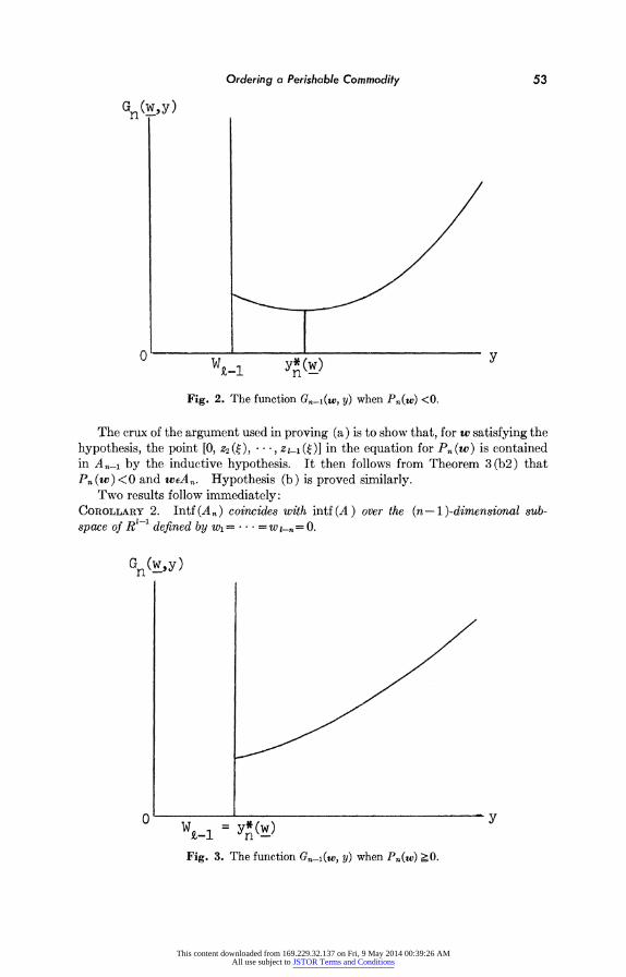
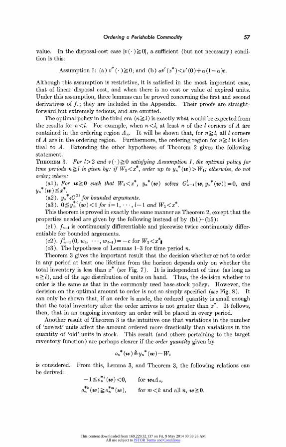
Returning to the proof, the function Gn-1 can be shown to be increasing for large values of y. Therefore, for each w a unique finite minimum of Gn1 (w, y) exists and is denoted Yn* (w). Figures 2 and 3 represent the two possible cases. These can be distinguished by evaluating the slope of the curve Gn-1 at the left boundary, where y = Wl. This quantity has been defined previously in (4) as Pn (w). For Pn (w) <0, the constrained minimum Yn* (w) occurs at the critical point, where G' -1 { w, Yn* (w) } = 0, and a positive order Yn* (w) - W1 is placed. When Pn (w) > 0, the minimum occurs at the left boundary Yn* (w) = W1, and no order is placed. Results (al) and (a2) follow immediately. The balance of the results follow from the application of the inverse-function theorem.

It has been shown that in the era 1 <n < 1 the target inventory does not depend on the immortal inventory [Theorem 2 (a5)]. The following corollaries deal with the relations between the ordering region and the immortal inventory. COROLLARY 1. For 1 <n <1, (a) if wO> is such that W-WI-n+l <xi* and W1 < x, then wEAn, (b) if w_O is such that Wi-Win+1< xi* and W1=xx*, then wEintf(An).




Gn (w,y)

0 y(wy U ~~WQ Y* (w)v

Fig. 2. The function Gn_l(w, y) when Pn(w) <0.

The crux of the argument used in proving (a) is to show that, for w satisfying the hypothesis, the point [0, Z2(h) * z** 1-1 (c)] in the equation for Pn (w) is contained in A,,- by the inductive hypothesis. It then follows from Theorem 3 (b2) that Pn (w) <0 and wEAR. Hypothesis (b) is proved similarly.

Two results follow immediately: COROLLARY 2. Intf (A,,) coincides with intf (A) over the (n- 1 )-dimensional sub- space of R-1' defined by w1 =* -w = =O.

Gn (w,y)

W' _ W y*(w)

Fig. 3. The function Gn-(w, y) when Pn(W) 20.



54 Brant E. Fries

COROLLARY 3. An contains at least n completed corners of A (including the corner at the origin).

These results, although they do not specify the ordering region completely, do suffice to give a general picture of its form. In period 1 (Fig. 1) the ordering region is the standard simplex with edge xi*. The following discussion is perhaps clarified by examining Figs. 4 and 5, which represent the ordering regions for 1 =4 when

WI

X

/ w \s

w 2

Fig. 4. The ordering region, 1 =4, n =2.

n = 2 and 3, respectively. In period 2, the ordering region has a completed corner on the W3 axis. In particular, if k*-x*-XI > , then using Corollary Il(b), any point w with WI-_n+,>k* is on the interface of A2. This represents the need to order when, for a given total inventory less than x*, the age distribution is heavily weighted toward the oldest units. It is necessary to begin purchasing in this period in order to prepare for future demand (in this case in the next period) when these oldest units will have expired. For the same total inventory less than x* in which there is a greater number of younger units, there are more units to satisfy demand




in future periods and it may be that no order need be placed. A similar logic ex- plains the form of the ordering region for n=3, where application of Corollary 1 now allows the inclusion in A3 of all of A except part of its corner on the w, axis.

The final corollary specifies a section of the ordering region where the order quantity is based on a single critical number: if an order is placed, order up to x*.

wJ1

x*\

I .\

1 X*

t1* w2

Fig. 5. The ordering region, 14, n =3.

Once again, let k* - x*l. The proof of this corollary follows almost immediately from the defining relation of yn* (w) and Corollary 1. COROLLARY 4. For 1<n<l, if w>O is such that Wln+?i?k* and Wi<x*, then Yn (w) = x*.

Figure 6 represents the target inventory function for units with a lifetime of three periods in the next-to-last period (n =2). The enclosed area on the base plane represents the ordering region A2, and the function Y2* (w) is shown only over that region [Y2* (w) = Wi for w outside the ordering region]. For age distributions with a large number of younger units it is not necessary to order units sufficient to bring the total inventory fully to x*. Instead, the purchasing of some units can



56 Brant E. Fries

be delayed for at least one period, and perhaps at that time ordering them will not be necessary. However, for age distributions weighted toward older units, a base- stock policy is followed, and y2* (w) = x* by Corollary 4. This higher level of inventory is necessary to protect against a large order at a later time to replace the oldest units, which will by then either have been issued or expired. A process of hedging is thus seen to be indicated. If a large number of units are due to expire

Y2 (w)

/s,/ 2 | 2

W i,

Fig. 6. The ordering region and the target inventory function for I=3, n =2

[Y2*(W) = W2 for w/A2].

in the near future, then units are ordered immediately; they serve the double purpose of bolstering the inventory immediately and also of attempting to forestall a large order in the future. If there are few units on hand, hedging leads to purchasing fewer units at this time and delaying the purchase of others to future periods.

The results of Theorem 2 and its corollaries hold when units have either a salvage value or a disposal cost. However, the assumptions about v ( ~) given above are insufficient to prove the existence of a similar optimal policy for n ? 1?>2 in both of these cost cases. An optimal value could not be found in the case of a salvage




value. In the disposal-cost case [v( )>0], a sufficient (but not necessary) condition is this:

Assumption I: (a) v"( )?0; and (b ) av' (x* ) <v' (O) +c a(1-o)c.

Although this assumption is restrictive, it is satisfied in the most important case, that of linear disposal cost, and when there is no cost or value of expired units. Under this assumption, three lemmas can be proved concerning the first and second derivatives of fn; they are included in the Appendix. Their proofs are straight- forward but extremely tedious, and are omitted.

The optimal policy in the third era (n ?_ 1) is exactly what would be expected from the results for n <1. For example, when n <1, at least n of the 1 corners of A are contained in the ordering region A,. It will be shown that, for n> 1, all 1 corners of A are in the ordering region. Furthermore, the ordering region for n > 1 is identical to A. Extending the other hypotheses of Theorem 2 gives the following statement. THEOREM 3. For 1>2 and v )_ 0 satisfying Assumption I, the optimal policy for time periods n? t is given by: if W1 <x*, order up to y *(w)> W1; otherwise, do not order; where:

(al). For w_O such that Wl<x*, yn*(w) solves G'_j{w,yn*(w)}=0, and

Yn w< (a2). yn*CC(l) for bounded arguments. (a3). O<y*'(w)<1 for i=1, , I-1 and WT<x*. This theorem is proved in exactly the same manner as Theorem 2, except that the

properties needed are given by the following instead of by (bi )- (b5): (cl). fn-, is continuously differentiable and piecewise twice continuously differ-

entiable for bounded arguments. (c2). f l-I (0, w2, * , w l1)= -c for W2< x*I (c3). The hypotheses of Lemmas 1-3 for time period n. Theorem 3 gives the important result that the decision whether or not to order

in any period at least one lifetime from the horizon depends only on whether the total inventory is less than x* (see Fig. 7). It is independent of time (as long as n > 1), and of the age distribution of units on hand. Thus, the decision whether to order is the same as that in the commonly used base-stock policy. However, the decision on the optimal amount to order is not so simply specified (see Fig. 8). It can only be shown that, if an order is made, the ordered quantity is small enough that the total inventory after the order arrives is not greater than x*. It follows, then, that in an ongoing inventory an order wi]l be placed in every period.

Another result of Theorem 3 is the intuitive one that variations in the number of 'newest' units affect the amount ordered more drastically than variations in the quantity of 'old' units in stock. This result (and others pertaining to the target inventory function) are perhaps clearer if the order quantity given by

?n (W) )- (W ) WI

is considered. From this, Lemma 3, and Theorem 3, the following relations can be derived:

-1-<on* (w ) <0, for WEAThn

OX;? (w) _ o*' (w) for <A; n 0*k (W) 0o-(W), frm<k and all n, w>O.



58 Brant E. Fries

Furthermore, it can be shown, again by tedious computation, that several of the inequalities of Lemma 3 hold strictly. In particular, the following Corollary can be proved. COROLLARY 4. For n _ 1, m <k, and wEA such that Wm,- Wk+l > O, then y*M (w) <

*k() and om(W) < O* (W).

W1

W3

W2 Fig. 7. The ordering region, 1=4, n >4.

It follows that for a given inventory a strictly larger order is placed if the age distribution is weighted toward older units than if the reverse is true. This is another example of the hedging discussed earlier, which applies for all n.

The result that the ordering region for n > 1 depends only on the total inventory and is independent of the age distribution leads one to question whether or not the same could be said for the target inventory function. This is not, however, the case. To specify the target inventory we need to know how many units of each age group are on hand-the total inventory and some of these values will not suffice.




Furthermore, it follows that the two most common simple inventory policies are not optimal. PROPOSITION 2. The ordering function y,* (w) for n? 1 cannot be represented for all w > 0 by a fu'rtion involving the total inventory W1 and a strict subset of the coordinates tWI, * WI-,

Yn -W

X*

wA I *~~~ =A

[y*(W) = W2for wjA].

PROPOSITION 3. Neither the 'single critical number' ('S) policy nor the 'two-bin' ['(s, S)'] policy is optimal for a perishable commodity when n ~1 > 2.

Proposition 2 can be proved by contradiction- using Corollary 4. If wi and wj are not explicitly included in the expression for the ordering function except through the total inventory, then the derivatives of y.* (w) taken with respect to each of these variables should be equal. The contradiction follows from Corollary 4. Proposition 3, in turn, follows directly from Proposition 2.



60 Brant E. Fries

ii. For 1= 2

The 1 = 2 case has not been combined with the 1> 2 case, since with 1-1 = 1 the notation of the proofs after that of Theorem 1 breaks down, and several statements such as Lemmas 2 and 3 do not apply. Nevertheless, the results and methods of proof are the same. The hypotheses given below are slightly more general than those of Van Zyl.11"5 Theorem 1 provides the optimal policy for n 1. In what follows, the constant x* is as defined before. THEOREM 4. For 1 = 2 and v (. ) 0 satisfying Assumption I, the optimal policy for time periods n ?2 is given by: if w1 <x*, order up to Yn* (w) > w1; otherwise do not order; where:

(al ). For w, < x*, Yn* (wl) satisfies G2-_I{w1, yn* (wi) } = 0, and yn* (wl) < X** (a2). Yn*C6l) for bounded arguments. (a3). OYn*(wl)<lforwi<x*.

PROPOSITION 4. Neither an S nor an (s, S) policy is optimal when n> 2.

CONCLUSION

THE PURPOSE OF this work was to present the form and properties of the exact optimal policy for a perishable commodity with lifetime 1 in a finite-horizon problem with continuous demand. Results have also been obtained for the steady-state optimal policy for the infinite-horizon model and for both the finite- and infinite- horizon models with discrete demand. Direct computation of optimal policies was accomplished and provided some further insight into the form of these policies. It is hoped that these extensions will be the subject of a future paper.

APPENDIX

LEMMA 1. In the disposal-cost case under Assumption I, for n = 0, 1, * *, 1 and j=1, * 1-1, fj (w)-v' (0) _ O for W1 <t, where t is the unique, finite solution to aL'(t)+aV'(t)-v'(0)=0. Equality may hold only when n=O. LEMMA 2. Forn<l andj= 1, . 1-2,fn 7(w)=f'; ' (w) if wIj=0. LEMMA 3. Let t be as in Lemma 1. For v( )> 0 satisfying Assumption I the following relations concerning the second partial derivatives of f. hold for n <1 (i, j, k, m=1, 2, *..,1-1):

(a) fnk'(w)> !Ofor WI-Wi<t. (b) fn k(W)-fn k(w)<0 for i<j<k and Wi-W3<t. (c) fnk(w)n 0k(w)>0for k<i<j and Wl-Wk<t.

(d) If" (W)_fnk(W) I_Ii-(W)_ f m(W)I>O for m<k<i<j and W1- Wk < t.

(e) y*" (w) -y*m (w) > 0 for m <k. The proofs of these lemmas can be found in Fries. [61




ACKNOWLEDGMENTS

AFTER WRITING THIS paper, I received details of similar work pursued concur- rently by STEVEN NAHMIAS at the University of Pittsburg.

I would like to thank the reviewers and Associate Editor EVAN L. PORTEUS for their help in identifying problems in clarity and presentation in an earlier draft.

REFERENCES

1. K. ARROW, S. KARLIN, AND H. SCARF, Studies in the Mathematical Theory of Inventory and Production, Stanford University Press, Stanford, California, 1958.

2. E. BARANKIN AND J. DENNY, Examination of an Inventory Model Incorporating Probabili- ties of Obsolescence, Technical Report 18, Statistical Laboratory, University of Cali- fornia, Berkeley, California, 1960.

3. G. BROWN, J. Lu, AND R. WOLFSON, "Dynamic Modeling of Inventory Subject to Ob- solescence," Management Sci. 11, 51-63 (1964).

4. E. BULINSKAYA, "Some Results Concerning Optimal Inventory Policies," Th. Prob. and its Appl. 9, 389-403 (1964).

5. H. EMMONS, "The Replenishment of Directly Used Radioactive Pharmaceuticals," Chapter 10 in The Optimal Use of Radioactive Pharmaceuticals in Medical Diagnosis, unpublished doctoral dissertation, Johns Hopkins University, Baltimore, Md., 1968.

6. B. FRIES, Optimal Ordering Policy for a Perishable Commodity with Fixed Lifetime, Tech- nical Report 148, Department of Operations Research, Cornell University, Ithaca, N.Y., 1972.

7. P. M. GHARE AND G. F. SHRADER, "A Model for Exponentially Decaying Inventory," J. Ind. Eng. 14, 238-243 (1963).

8. G. HADLEY AND T. M. WHITIN, "An Optimal Final Inventory Model," Management Sci. 7, 179-183 (1961).

9. , "Generalizations of the Optimal Final Inventory Model," Management Sci. 8, 454-457 (1962).

10. M. IGEL, "Een Dynamische Seviegrootteberebening" ("Dynamic Computation of Order Size") Tijdschrift voor Efficientie en Documentatie (Neth.) 35, 169-173 (1965); abstracted in I.A.O.R. 5, 259, No. 3527 (1965).

11. D. L. IGLEHART AND S. C. JAQUETTE, "Multi-class Inventory Models with Demand a Function of Inventory Level," Naval Res. Logist. Quart. 16, 495-502 (1969).

12. J. B. JENNINGS, "Blood Bank Inventory Control," Management Sci. 19, 637-645 (1973). 13. G. R. MURRAY, JR. AND E. A. SILVER, "A Bayesian Analysis of the Style Goods Inven-

tory Problem," Management Sci. 12, 785-797 (1966). 14. W. PIERSKALLA, "An Inventory Problem with Obsolescence," Naval Res. Logist. Quart.

16, 217-228 (1969). 15. G. J. J. VAN ZYL, Inventory Control for Perishable Commodities, unpublished doctoral

dissertation, Univ. of North Carolina, Chapel Hill, N.C., 1964.



optimal ordering policy for a perishable commodity with fixed lifetime

Documents