optimal ordering, discounting, and pricing in the single-period problem

*Tel.: 001-704-547-3242; fax: 001-704-547-3123.E-mail address: [email protected] (M.J. Khouja)

Int. J. Production Economics 65 (2000) 201}216

Optimal ordering, discounting, and pricing in the single-periodproblem

Moutaz J. Khouja*

Information & Operations Management Department, The Belk College of Business Administration,The University of North Carolina at Charlotte, Charlotte, NC 28223, USA

Received 22 October 1998; accepted 23 March 1999

Abstract

The single-period problem (SPP), also known as the newsboy or newsvendor problem, is to "nd the order quantitywhich maximizes the expected pro"t in a single-period probabilistic demand framework. Previous extensions to the SPPinclude, in separate models, the simultaneous determination of the optimal price and quantity when demand isprice-dependent, and the determination of the optimal order quantity when progressive discounts with preset prices areused to sell excess inventory. In this paper, we extend the SPP to the case in which demand is price-dependent andmultiple discounts with prices under the control of the newsvendor are used to sell excess inventory. First, we develop twoalgorithms for determining the optimal number of discounts under "xed discounting cost for a given order quantity andrealization of demand. Then, we identify the optimal order quantity before any demand is realized. We also analyze thejoint determination of the order quantity and initial price. We illustrate the models and provide some insights usingnumerical examples. ( 2000 Elsevier Science B.V. All rights reserved.

Keywords: Inventory management; Production management; Operations management

1. Introduction

The classical single-period problem (SPP) is to"nd a product's order quantity which maximizesthe expected pro"t in a probabilistic demandframework. The SPP model assumes that if anyinventory remains at the end of the period, onediscount is used to sell it or it is disposed of [1]. Ifthe order quantity is smaller than the realized de-mand, the newsvendor, hereafter NV, forgoes some

pro"t. If the order quantity is larger than the realiz-ed demand, the NV losses some money becausehe/she has to discount the remaining inventory toa price below cost. The SPP is re#ective of manyreal-life situations and is often used to aid decisionmaking in the fashion and sporting industries, bothat the manufacturing and retail levels [2]. The SPPcan also be used in managing capacity and evaluat-ing advanced booking of orders in service indus-tries such as airlines, hotels, etc. [3].

Several researchers have suggested SPP exten-sions in which demand is price dependent [4}10].Whitin [4] assumed that the expected demand isa function of price and using incremental analysis,derived the necessary optimality condition. He then

0925-5273/00/$ - see front matter ( 2000 Elsevier Science B.V. All rights reserved.PII: S 0 9 2 5 - 5 2 7 3 ( 9 9 ) 0 0 0 2 7 - 4

provided closed-form expressions for the optimalprice, which is used to "nd the optimal orderquantity for a demand with a rectangular distribu-tion. Mills [5] also assumed demand to be a ran-dom variable with an expected value that isdecreasing in price and with constant variance.Mills derived the necessary optimality conditionsand provided further analysis for the case of de-mand with rectangular distribution.

Lau and Lau (LL) [6] introduced a model inwhich the NV has the option of decreasing price inorder to increase demand. LL analyzed two casesfor demand:

(a) Case A: Demand is given by a simple homo-scedastic regression model x"a!bP#e, wherea and b are constants, x is the quantity demanded,P is unit price, and e is normally distributed. Theabove equation implies a normally distributed de-mand with an expected value which decreases lin-early with unit price.

(b) Case B: Demand distribution is constructedusing a combination of statistical data analysis andexperts' subjective estimates. The &method of mo-ments' was used to "t the four-parameter beta dis-tribution to estimate demand.

For case A, LL showed that the expected pro"t isunimodal and thus the golden section method canbe used for maximization. For case B, there is noguarantee the expected pro"t is unimodal. Thus,LL developed a search procedure for identifyinglocal maximums. LL also solved the problem underthe objective of maximizing the probability ofachieving a target pro"t and considered both zeroand positive shortage cost cases. For zero shortagecost and demand given by case A, LL derivedclosed-form solutions for the optimal order quanti-ty and optimal price. For zero shortage cost anddemand given by case B, LL developed a procedurefor computing the probability of achieving a targetpro"t and used a search procedure for "ndinga good solution. For positive shortage cost anddemand given by cases A or B, the probability ofachieving a target pro"t may not be unimodal. LLdeveloped procedures for computing the probabil-ity of achieving a target pro"t and identifyinga good solution.

Polatoglu [7] also considered the simultaneouspricing and procurement decisions. Polatoglu

identi"ed few special cases of the demand processaddressed in the literature: (i) an additive model inwhich the demand at price P is x(P)"k(P)#e,where k(P) is the mean demand as a function ofprice, and e is a random variable with a knowndistribution and E[e]"0, (ii) a multiplicativemodel in which x(P)"k(P)e where E[e]"1, (iii) ariskless model in which X(P)"k(P). Polatogluanalyzed the SPP under general demand uncertain-ty to reveal the fundamental properties of themodel independent of the demand pattern.Polatoglu assumed an initial inventory of I, k(P)is a monotone decreasing function of P on(0, R), and a "xed ordering cost of k. For linearexpected demand, (k(P)"a!bP, where a, b'0)Polatoglu proved the unimodality of the expectedpro"t for uniformly distributed additive demandand exponentially distributed multiplicativedemand.

Khouja [8] solved an SPP in which multiplediscounts are used to sell excess inventory. In thismodel, retailers progressively increase the discountuntil all excess inventory is sold. The product isinitially o!ered at the regular price P

0. After some

time, if any inventory remains the price is reducedto P

1, P

0'P

1. In general, the prices are

Pi, i"0, 1,2, n, where P

i'P

i`1. The amount de-

manded at each Pi

is assumed to be a multipleti, i"1,2, n of the demand at the regular price P

0.

Khouja solved the problem under two objectives:(a) maximizing the expected pro"t, and (b) maxi-mizing the probability of achieving a target pro"t.Khouja showed that the expected pro"t is concaveand derived the su$cient optimality condition forthe order quantity. For maximizing the probabilityof achieving a target pro"t, Khouja providedclosed-form expression for the optimal orderquantity. Khouja [10] developed an algorithm foridentifying the optimal order quantity for themulti-discount SPP when the supplier o!ers theNV an all-units quantity discount. Khouja andMehrez [9] provided a solution algorithm to themulti-product multi-discount constrained SPP.

The above models may not capture some actualproblems facing many NVs. While NV may con-sider the demand}price relationship is determiningthe order quantity, he/she still faces the problem ofwhat to do with excess inventory when the order

202 M.J. Khouja / Int. J. Production Economics 65 (2000) 201}216

quantity exceeds the realized demand. Mostretailers, for example, do not use a single discountto sell excess inventory as assumed in the classicalSPP. The assumption of multiple discounts pro-posed by Khouja [8] contributes a step towardsolving this problem. However, Khouja's model islimited in that it assumes that the discount pricesare preset and are not part of the decisions ofthe NV. The model also assumes that the quantitysold at each discount price is a given multiple ofthe quantity sold at the initial price without anyassumptions about demand}price relationship.Finally, the model assumes that discountinga product does not incur a "xed cost, whereasmany retailers incur a "xed discounting costresulting from the need to advertise the dis-count and markdown the discounted items. Inthis paper, we extend the SPP to the case inwhich:

1. demand is price dependent,2. multiple discount prices are used to sell excess

inventory,3. the discount prices used to sell excess inventory

are under the control of the NV, and4. there is a positive setup cost associated with

discounting a product due to the costs of advert-ising and marking down the discounted items.

The resulting problem is composed of two small-er problems. In the "rst problem, for a given realiz-ation of demand, a given demand}price relation-ship, and a given order quantity, the NV mustdetermine the optimal discounting scheme. Thisproblem will be referred to as the discounting prob-lem. In the second problem, the NV must determinethe order quantity which maximizes the expectedpro"t prior to any demand being realized. Thisproblem will be referred to as the order quantityproblem.

In the next section, we review the classical SSP.In Section 3, we analyze the discounting problemand develop two algorithms for determining theoptimal discounting scheme under two di!erentassumptions about the behavior of the NV. InSection 4, we solve the optimal order quantityproblem. In Section 5, we analyze the joint quantity

and initial pricing decisions. We conclude in Sec-tion 6.

2. Basic results and problem motivation

De"ne the following notation:x "quantity demanded, a random variable,f (x)"the probability density function of x,F(x)"the cumulative distribution function of x,P "per unit selling price,C "per unit cost,< "per unit salvage value,S "per unit shortage penalty cost,C

0"C!<, per unit overage cost,

C6

"P!C#S, per unit underage cost, andQ "order quantity, a decision variable.

The pro"t per period is

n"G(P!C)Q!S(x!Q) if x*Q,

Px#<(Q!x)!CQ if x(Q.(1)

Simplifying and taking the expected value of n givesthe following expected pro"t:

E(n)"(P#S!C)P=

Q

Qf (x) dx!SP=

Q

xf (x) dx

#(P!<)PQ

0

xf (x) dx!(C!<)PQ

0

Qf (x) dx.

(2)

Let the superscript H denote optimality. UsingLeibniz's rule to obtain the "rst and second deriva-tives of E(n) shows that it is concave, and thus, thesu$cient optimality condition is to set the "rstderivative to zero which yields the well-known frac-tile formula:

F(QH)"P#S!C

P#S!<. (3)

Suppose the NV uses multiple discounts to sellexcess inventory. In this case, the SPP decomposesinto two problems: the discounting problem andthe order quantity problem. The sequence of eventsin the SPP is as follows: (1) The NV sets the initialprice at which to o!er the product (P

0) based on the

M.J. Khouja / Int. J. Production Economics 65 (2000) 201}216 203

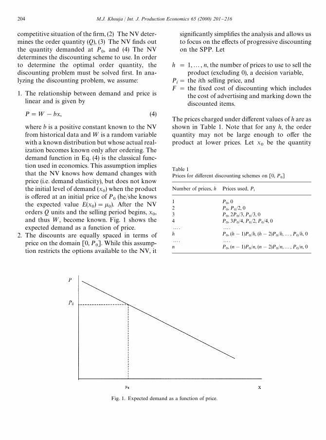
Fig. 1. Expected demand as a function of price.

Table 1Prices for di!erent discounting schemes on [0, P

0]

Number of prices, h Prices used, Pi

1 P0, 0

2 P0, P

0/2, 0

3 P0, 2P

0/3, P

0/3, 0

4 P0, 3P

0/4, P

0/2, P

0/4, 0

2. 2.h P

0, (h!1)P

0/h, (h!2)P

0/h,2, P

0/h, 0

2. 2.n P

0, (n!1)P

0/n, (n!2)P

0/n,2, P

0/n, 0

competitive situation of the "rm, (2) The NV deter-mines the order quantity (Q), (3) The NV "nds outthe quantity demanded at P

0, and (4) The NV

determines the discounting scheme to use. In orderto determine the optimal order quantity, thediscounting problem must be solved "rst. In ana-lyzing the discounting problem, we assume:

1. The relationship between demand and price islinear and is given by

P"=!bx, (4)

where b is a positive constant known to the NVfrom historical data and= is a random variablewith a known distribution but whose actual real-ization becomes known only after ordering. Thedemand function in Eq. (4) is the classical func-tion used in economics. This assumption impliesthat the NV knows how demand changes withprice (i.e. demand elasticity), but does not knowthe initial level of demand (x

0) when the product

is o!ered at an initial price of P0

(he/she knowsthe expected value E(x

0)"k

0). After the NV

orders Q units and the selling period begins, x0,

and thus =, become known. Fig. 1 shows theexpected demand as a function of price.

2. The discounts are equally spaced in terms ofprice on the domain [0, P

0]. While this assump-

tion restricts the options available to the NV, it

signi"cantly simpli"es the analysis and allows usto focus on the e!ects of progressive discountingon the SPP. Let

h " 1,2, n, the number of prices to use to sell theproduct (excluding 0), a decision variable,

Pi" the ith selling price, and

F " the "xed cost of discounting which includesthe cost of advertising and marking down thediscounted items.

The prices charged under di!erent values of h are asshown in Table 1. Note that for any h, the orderquantity may not be large enough to o!er theproduct at lower prices. Let x

0be the quantity


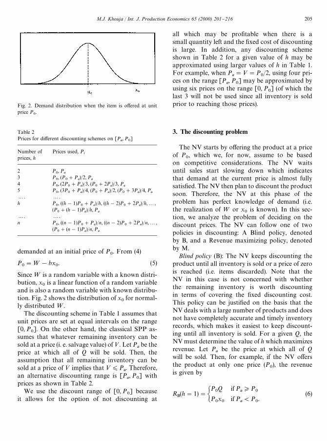
Fig. 2. Demand distribution when the item is o!ered at unitprice P

0.

Table 2Prices for di!erent discounting schemes on [P

a, P

0]

Number ofprices, h

Prices used, Pi

2 P0, P

a3 P

0, (P

0#P

a)/2, P

a4 P

0, (2P

0#P

a)/3, (P

0#2P

a)/3, P

a5 P

0, (3P

0#P

a)/4, (P

0#P

a)/2, (P

0#3P

a)/4, P

a2. 2.h P

0, ((h!1)P

0#P

a)/h, ((h!2)P

0#2P

a)/h,2,

(P0#(h!1)P

a)/h, P

a2. 2.n P

0, ((n!1)P

0#P

a)/n, ((n!2)P

0#2P

a)/n,2,

(P0#(n!1)P

a)/n, P

a

demanded at an initial price of P0. From (4)

P0"=!bx

0. (5)

Since= is a random variable with a known distri-bution, x

0is a linear function of a random variable

and is also a random variable with known distribu-tion. Fig. 2 shows the distribution of x

0for normal-

ly distributed=.The discounting scheme in Table 1 assumes that

unit prices are set at equal intervals on the range[0, P

0]. On the other hand, the classical SPP as-

sumes that whatever remaining inventory can besold at a price (i. e. salvage value) of<. Let P

abe the

price at which all of Q will be sold. Then, theassumption that all remaining inventory can besold at a price of < implies that <)P

a. Therefore,

an alternative discounting range is [Pa, P

0] with

prices as shown in Table 2.We use the discount range of [0, P

0] because

it allows for the option of not discounting at

all which may be pro"table when there is asmall quantity left and the "xed cost of discountingis large. In addition, any discounting schemeshown in Table 2 for a given value of h may beapproximated using larger values of h in Table 1.For example, when P

a"<"P

0/2, using four pri-

ces on the range [Pa, P

0] may be approximated by

using six prices on the range [0, P0] (of which the

last 3 will not be used since all inventory is soldprior to reaching those prices).

3. The discounting problem

The NV starts by o!ering the product at a priceof P

0, which we, for now, assume to be based

on competitive considerations. The NV waitsuntil sales start slowing down which indicatesthat demand at the current price is almost fullysatis"ed. The NV then plan to discount the productsoon. Therefore, the NV at this phase of theproblem has perfect knowledge of demand (i.e.the realization of = or x

0is known). In this sec-

tion, we analyze the problem of deciding on thediscount prices. The NV can follow one of twopolicies in discounting: A Blind policy, denotedby B, and a Revenue maximizing policy, denotedby M.

Blind policy (B): The NV keeps discounting theproduct until all inventory is sold or a price of zerois reached (i.e. items discarded). Note that theNV in this case is not concerned with whetherthe remaining inventory is worth discountingin terms of covering the "xed discounting cost.This policy can be justi"ed on the basis that theNV deals with a large number of products and doesnot have completely accurate and timely inventoryrecords, which makes it easiest to keep discount-ing until all inventory is sold. For a given Q, theNV must determine the value of h which maximizesrevenue. Let P

abe the price at which all of Q

will be sold. Then, for example, if the NV o!ersthe product at only one price (P

0), the revenue

is given by

RB(h"1)"G

P0Q if P

a*P

0P0x0

if Pa(P

0.

(6)


RB(h"4)"G

P0Q if P

a*P

0,

P0x0#(3P

0/4)(Q!x

0)!F if 3P

0/4)P

a(P

0,

P0x0#(3P

0/4)(P

0/4b)#(P

0/2)(Q!P

0/4b!x

0)!2F if 2P

0/4)P

a(3P

0/4,

P0x0#(3P

0/4)(P

0/4b)#(P

0/2)(P

0/4b)

#(P0/4)(Q!P

0/2b!x

0)!3F if P

0/4)P

a(2P

0/4,

P0x0#(3P

0/4)(P

0/4b)#(P

0/2)(P

0/4b)

#(P0/4)(P

0/4b)!3F if P

a(P

0/4.

Simplifying gives

RB(h"4)"G

P0Q if P

a*P

0,

(3P0/4)Q#(P

0/4)x

0!F if 3P

0/4)P

a(P

0,

(2P0/4)Q#(2/4)P

0x0#P2

0/16b!2F if 2P

0/4)P

a(3P

0/4,

(P0/4)Q#(3P

0/4)x

0#3P2

0/16b!3F if P

0/4)P

a(2P

0/4,

P0x0#6P2

0/16b!3F if P

a(P

0/4.

(7)

In general, for any number of prices h, the revenue is given by

RB"G

P0Q if P

a*P

0,

j

hP0x0#

h!j

hP0Q#

P20

bh2j~1+i/0

i!jF ifh!j

hP0)P

a(

h!j#1

hP0,

P0x0#

P20

bh2h~1+i/0

i!(h!1)F if Pa(

P0

h.

(8)

If the NV o!ers the product at four prices(P

0, 3P

0/4, 2P

0/4, and P

0/4) then, using (5), the

incremental quantity demanded at each dis-count price is P

0/4b and the revenue is given

by

Obviously, if Pa'P

0(or equivalently Q(x

0) then

no discounts are needed and hH"1. De"ne k as

k"maxGh:h!1

hP0)P

a(P

0H.In other words, k is the largest number of priceswhich satis"es [(k!1)/k]P

0)P

a. Lemmas 1 and

2 are introduced to develop an algorithm which cane$ciently identify hH.

Lemma 1. The optimal number of prices at which toower the product satisxes hH*k.

Proof. The proof of Lemma 1 is provided in theappendix.

Lemma 2. For any number of prices v such thatv'k and for any integer j, if

v!j

vP0)P

a(

v!j#1

vP

0and

v#1!j

v#1P0)P

a(

v!j#2

v#1P

0,

then the revenue from using h"v#1 is greater thanor equal to the revenue from using h"v (i.e.R

B(v#1)*R

B(v)).


Algorithm 1: Blind policy

Step 1: Compute Pa

using (4). If Pa*P

0then

stop, all of Q will be sold at the initial price P0.

Step 2: Find the largest h for which [(h!1)/h]P0)P

a(P

0. Denote this h as k.


If k"n then stop k is optimal. (by Lemma 1)Set i"nStep 3: Find the largest integer, j, for which

[(i!j)/i]P0)P

a([(i!j#1)/i]P

0.

If [(i!j!1)/(i!1)]P0)P

a([(i!j)/(i!1)]P

0,

then h"i!1 is suboptimal. (by Lemma 2)Step 4: Set i"i!1.If i'k#1 go to Step 3.Compute revenue using (8) for h"k and all

h'k not found to be suboptimal.Select h with the largest revenue.

Steps 1 and 2 are performed once. Step 2 requiresmore computations than Step 1 and is bounded byn. In the worst case, Step 3 is performed n times andeach of these iterations is bounded by n. Finally,Step 4 is bounded by n. Therefore, the running timeof the algorithm is O(n2).

Revenue maximizing policy (Policy M): Here, thelast discount (j) for a given number of prices (h) iso!ered only if the additional revenue from it isgreater than or equal to the "xed cost of discount-ing (F). Thus, if (h!j)P

0/h)P

a((h!j#1)P

0/h

then discount j is used only if the additional rev-enue it generates from selling the additional unitsdemanded between prices (h!j)P

0/h and P

ais

greater than or equal to F. To simplify the analysis,we introduce the following realistic assumption:

Assumption 1. The largest number of prices the NVmay use (n), is such that the incremental revenuefrom selling all units demanded between prices2P

0/n and P

0/n is greater than F.

In other words, the NV will not use prices soclose to each other to the point where the incremen-tal revenue of a discount is insu$cient to cover the"xed cost of the discount. From (5) the quantitiessold at 2P

0/n and P

0/n are (=!P

0/n)/b and

(=!2P0/n)/b, respectively. Thus, the incremental

units sold at P"P0/n are P

0/nb and the incremen-

tal revenue is (P0/nb)P

0/n"P2

0/bn2. Assumption

1 can be restated as

P20

bn2*F. (9)

In order to derive the revenue function underthis policy, we need to introduce a new policy,denoted C. Suppose that discount j is not usedunless the full quantity demanded at that discountprice is available. When the quantity available atdiscount j is small, the "xed cost of discounting willbe greater than the incremental revenue from sell-ing this small quantity. Thus, discounting will re-duce revenue and R

C'R

B. When the quantity

available at discount j is large (but insu$cient tosatisfy all of the incremental demand at that price),the "xed cost of discounting will be smaller than theincremental revenue from selling this large quanti-ty. Thus, discounting will increase revenue andR

C(R

B. To obtain R

C, the revenue from the last

discount is eliminated from the expression forR

Band the coe$cient of F is reduced by one. For

example, the revenue functions for h"2 and 4 inpolicy C are:

RC(h"2)"G

P0Q if P

a*P

0,

P0x0

if P0/2)P

a(P

0,

P0x0#P2

0/4b!F if P

a(P

0/2.

(10)

and

RC(h"4)"G

P0Q if P

a*P

0,

P0x0

if 3P0/4)P

a(P

0,

P0x0#3P2

0/16b!F if 2P

0/4)P

a(3P

0/4,

P0x0#5P2

0/16b!2F if P

0/4)P

a(2P

0/4,

P0x0#6P2

0/16b!3F if P

a(P

0/4.

(11)


In general, for any h, RC

is given by

RC"G

P0Q if P

a*P

0,

P0x0

ifh!1

hP

0)P

a(P

0,

P0x0#

P20

bh2

h~1+

i/h~j`1

i!( j!1)F ifh!j

hP0)P

a(

h!j#1

hP

0,

P0x0#

P20

bh2h~1+i/1

i!(h!1)F if Pa(

P0

h.

(12)

From (8) and (12), the di!erence in revenue between the Blind policy and policy C is

RB!R

C"G

0 if P0*P

a,

h!1

hP0(Q!x

0)!F if

h!1

hP0)P

a(P

0,

h!j

hP

0(Q!x

0)#

P20

bh2 Cj~1+i/0

i!h~1+

i/h~j`1

iD!F ifh!j

hP

0)P

a(

h!j#1

hP0,

0 if Pa(

P0

h.

(13)

Let RM

be the revenue of the Revenue Maximizingpolicy, (R

B!R

C) will be used to "nd h which maxi-

mizes RM. For a given Q and h, if (R

B!R

C)'0

then the last discount should be used and RM"R

B.

If (RB!R

C)(0 then the last discount should not

be used and RM"R

C. Because under the Revenue

Maximizing policy the last discount may or maynot be used we must "nd both hH and jH. Note thath and hH are used to denote the number of pricesand the optimal number of prices, respectively, forboth the B and M policies. Using the de"nition ofk introduced before Lemma 1, Lemma 3 introducesimportant properties of R

M.

Lemma 3. The optimal number of prices at which toower the product satisxes hH*k or hH"1.

Proof.The proof of Lemma 3 is provided in theappendix.

Algorithm 2: Revenue maximizing policy

Step 1. Compute Pa

using (4). If Pa*P

0then

stop, all of Q will be sold at the initial price P0.

Step 2. Find the largest h for which [(h!1)/h]P0)P

a(P

0. Denote this h as k.

If k"n and [(k!1)/k]P0(Q!x

0)'F then stop

hH"k and jH"1.If k"n and [(k!1)/k]P

0(Q!x

0)(F then stop

hH"k and jH"0.If k(n and [(k!1)/k]P

0(Q!x

0)'F then

RM(k) is given by (8).If k(n and [(k!1)/k]P

0(Q!x

0)(F then

RM(k) is given by (12).Set h"k#1Step 3. Find the largest integer, j, for which

[(h!j)/h]P0)P

a([(h!j#1)/h]P

0.

If

h!j

hP0(Q!x

0)#

P20

bh2 Cj~1+i/0

i!h~1+

i/h~j`1

iD'F

then RM(h) is given by (8) otherwise R

M(h) is given

by (12).Step 4. Set h"h#1.If h(n go to Step 3.Compute R

M(h) using the function constructed in

Steps 2 and 3 for all h*k.Select h with the largest revenue.

Similar to Algorithm 1, Steps 1 and 2 are performedonce. Step 2 requires more computations and


RM"G

0.5P0x0#0.5P

0Q!F"$206,700 if h"2,

P0x0#2P2

0/bh2!F"$208,089 if h"3,

2P0x0/4#2P

0Q/4#P2

0/bh2!2F"$208,400 if h"4,

2P0x0/5#3P

0Q/5#P2

0/bh2!2F"$209,000 if h"5,

3P0x0/6#3P

0Q/6#3P2

0/bh2!3F"$208,433 if h"6,

3P0x0/7#4P

0Q/7#3P2

0/bh2!3F"$208,620 if h"7.

(14)

is bounded by n. In the worst case, Step 3 is per-formed n times and each of these iterations isbounded by n. Finally, Step 4 is bounded by n.Therefore, the running time of the algorithm is O(n2).

Numerical Example 1. Consider a product withdemand function P"=!0.01x, where= is nor-mally distributed with a mean of 110 and a stan-dard deviation of 10. This implies an increase of 100units in demand for each $1 drop in price. The "xedcost of discounting is F"$800. Suppose the NVordered Q"10,750 units and is using the Blind

policy. The NV o!ered the product at an initialprice of P

0"$20 and found that the realization for

= was 120 or equivalently x0"10,000 units The

question facing the NV is how many prices to use tosell all of Q? The NV limits the number of possibleprices at which to o!er the product to n"7 whichsatis"es assumption 1. Thus, the choice of h must tobe made from h"1, 2,2, 7. Using (4), the price atwhich all of the 10,750 units will be sold isPa"$12.5. Algorithm 1 shows that one of the

values of h"2, 5, or 7 is optimal. Using (8) withQ"10,750 gives R

B(h"2)"$206,700, R

B(h"5)"

$209,000, and RB(h"7)"$208,620 and thus,

hH"5, which corresponds to discounts of20% from the original price and unit prices of$20.00, $16.00, $12.00, $8.00, and $4.00. The lastunit in Q"10,750 will be sold for $12.00. If thevalue of b is changed to b"0.02, which implies a 50unit increase in demand for each $1 drop in unitprice, and the realization of = is changed to="220, then the realized demand at P

0"$20

remains x0"10,000. However, the optimal

number of prices decreases to hH"4 withR

B(h"4)"$205,100. Because the additional

quantity sold at each discount is smaller with thenew b, then it is optimal to use smaller number ofprices and larger discounts. If the value of Fis changed to F"$3,200 then it is optimal touse hH"2 for which R

B(h"2)"$204,300.

Because the cost of discounting is higher, it is opti-mal to use a smaller number of prices and largerdiscounts.

Now suppose the NV is using a Revenue Maxi-mizing policy. The application of Algorithm 2 forQ"10,750 and P

a"$12.50 results in the following

revenue function:

Thus, hH"5, jH"2, RHM"RH

B"$209,000 and

the Blind and the Revenue Maximizing policygive the same results. For Q"10,680, P

a"$13.2

and the Blind policy gives hH"5, andRH

B"$208,160 whereas the Revenue Maximizing

policy gives hH"6, jH"2, and RHM"$208,400

which corresponds to discounts of 16.67% from theinitial price.

4. The order quantity problem

We start by assuming that the initial selling priceis preset with value that depends on the competitivesituation of the "rm. We focus our attention on theBlind policy since dealing with the Revenue maxi-mizing policy is complex and will distract us fromour purpose of analyzing the e!ects of multiplediscounts on the optimal order quantity and initialprice. For the order quantity problem, the NV onlyknows the distribution (i.e. the mean, standard de-viation and distributional form) of demand at dif-ferent prices. From (8), the expected pro"t for


a given h is

E(n(h))"P=

Q

P0Q f (x

0) dx

0

#

h~1+j/1P

Q~(j~1)P0@hb

Q~jP0@hbC

j

hP0x0#

h!j

hP0Q

#

P20

bh2

j~1+i/0

i!jFD f (x0) dx

0

#PQ~(h~1)P0@hb

0CP0

x0#

P20

bh2h~1+i/0

i

!(h!1)FD f (x0) dx

0!CQ. (15)

We simplify (15) and "nd QH for normally anduniformly distributed demand.

4.1. Uniform demand distribution

Suppose x0

is uniformly distributed on the range[a, b], then Eq. (15) gives

E(n(h))

"

1

b!a CP0

2hA!hQ2#2hQb!ha2!P2

0S1

h2b2B#

P20S2

h2b(Q!a)

!(h!1)FAQ!a#P

0S3

h(h!1)bB!CQ(b!a)D,(16)

where

S1"

h~1+i/0

i2, S2"

h~1+i/0

i, and S3"

h~2+i/0

i.

Lemma 4 provides proof of concavity of E(n(h)).Setting dE(n(h))/dQ"0 yields QH

hfor a given h:

QHh"b#

P0

h2b

h~1+i/0

i!(h!1)F#C(b!a)

P0

. (17)

Lemma 4. The expected proxt function is concave inQ for uniformly distributed demand.


Thus, to obtain the optimal order quantity (QH),the optimal order quantities for all values of h (i.e.QH

h, h"1,2, n) are computed using (17) and then

E(n(h)) for each QHh

is computed using (16). Byenumerating over all h"1, 2,2, n we identify theQH

hthat maximizes E(n(h)).

4.2. Normal demand distribution

Suppose x0

is normally distributed with meank0and standard deviation p. From (15), the revenue

for a given h is

E(n(h))"P`=

Q

P0Q f (x

0) dx

0

#

h~1+j/1

PQ~(j~1)P0@hb

Q~jP0@hbAjP

0x0

h#

(h!j)P0Q

h

#

P20

bh2S2!jFB f (x

0) dx

0

#PQ~(h~1)P0@hb

~=AP0

x0#

P20

bh2S2

!(h!1)FB f (x0) dx

0. (18)

Our analysis indicates that E(n(h)) is concave fordi!erent values of h. However, we are able to provethat QH

his in the concave region of E(n(h)) only

under the conditions stated in Lemma 5. De"nePk

as the highest price for which Pk)C for a

given h.

Lemma 5. If F#C!Pk`1

*k(P0!C) and

kP20)b2h2p2, then for normally distributed demand

dE(n(h))/dQ"0 is a suzcient condition for opti-mality.


Setting dE(n(h))/dQ"0, gives the su$cient opti-mality condition:

P0

h Ch!h~1+i/0

F AQ!

iP0

hb BD!Fh~2+i/0

f AQ!

iP0

hb B!C"0, (19)


Table 3Optimal order quantities and expected pro"t for di!erent dis-counting schemes and uniform demand distribution

h QHh

E(n(h))

1 10000 $90,000.002 10460 $93,879.003 10587 $94,741.934H 10630 $94,804.755 10640 $94,544.006 10633 $94,123.157 10617 $93,613.39

Table 4Optimal order quantities and expected pro"t for di!erent dis-counting schemes and normal demand distribution

h QH E(n(h))

1 10000 $91,999.972 10459 $95,466.633 10582 $96,550.644 10622 $96,939.175* 10631 $97,043.676 10623 $97,007.847 10607 $96,894.11

which can be solved using a simple search proced-ure. Now QH

h, h"1,2, n and their corresponding

E(n(h)) are computed and the best QHh

is ordered.Evaluating E(n(h)) requires numerical integration.

Numerical Example 2. Reconsider Example 1 with= uniformly distributed on [100, 140] which im-plies that x

0is uniformly distributed with a"8,000

and b"12,000 for P0"$20. Using Eqs. (16) and

(17) gives the results in Table 3. Thus, the optimalnumber of prices is hH"4, QH"10,630 andE(n(h))"$94,804.75. After the order is placed anddemand becomes known, the application of Algo-rithm 1 may result in a new value of hH at thediscounting problem. For smaller cost of discount-ing of F"$200, the solution changes tohH"7, QH"10,797 and E(n(h))"$96,692.67.

Suppose= is normally distributed with a meanof E(=)"120 and standard deviation p(=)"10which implies that x

0is normally distributed with

mean k0"10,000 and standard deviation

p"1,000 for P0"$20. Using Eqs. (18) and (19)

gives the results in Table 4. Thus, the optimalnumber of prices is hH"5, QH"10,631, andE(n(h))"$97,043.67.

5. Optimal initial price

In this case, initial unit o!ering price (P0) is

a decision variable and the NV must determine theoptimal values of both Q and P

0. We analyze the

case of uniformly distributed demand (i.e.x0&U[a, b]) and provide closed-form solution for

it. Using P0"C with the expressions for a and

b gives the minimum and maximum possible de-mands, (=

1!C)/b and (=

2!C)/b, respectively, if

the product is o!ered at cost. Let

a1"

1

b2 AS1

2h3#

1

2!

S2

h2B, (20)

a2"

1

b AQ!

=1

b B A1!S2

h2B, (21)

a3"

1

2(Q2#=2

1)#

F

b AS3h#h!1B!

Q=2

b(22)

and

a4"(h!1)F A

=1

b!QB!

CQ

b(=

2!=

1). (23)

Substituting from (20)}(23) into (16) gives

E(n(h))"b

=2!=

1

[a4!a

3P0!a

2P20!a

1P30].

(24)

The derivative of E(n(h)) with respect to P0

is

LE(n(h))

LP0

"

!b

=2!=

1

[a3#2a

2P0#3a

1P20] (25)

with roots at

P01

, P02"

!2a2$Ja2

2!12a

1a3

6a1

. (26)

Substituting di!erent values of h into (20) showsthat a

1'0. If a

2'0 then (26) gives one negative

root and one positive root independent of the value


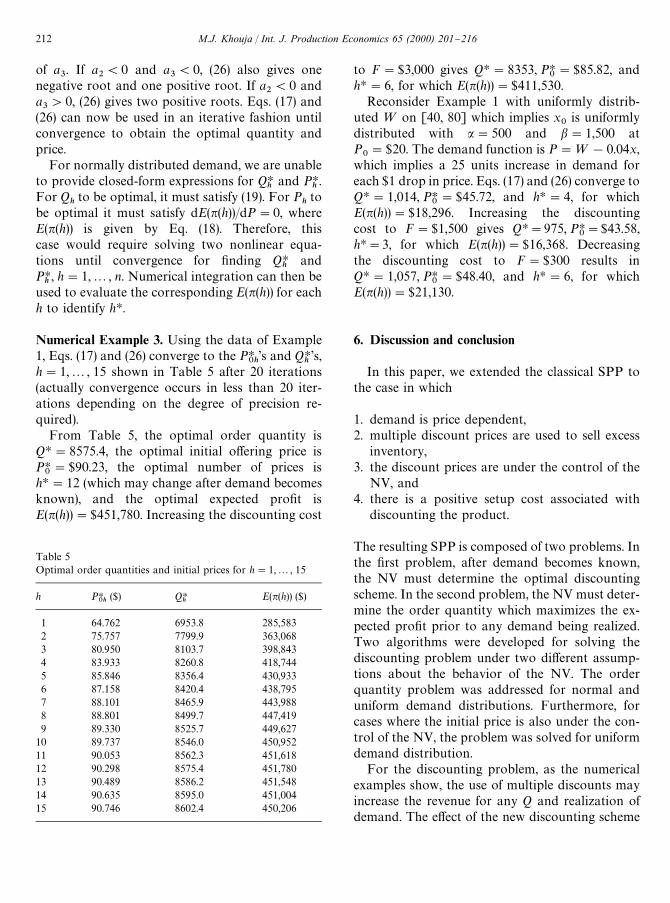
Table 5Optimal order quantities and initial prices for h"1,2, 15

h PH0h

($) QHh

E(n(h)) ($)

1 64.762 6953.8 285,5832 75.757 7799.9 363,0683 80.950 8103.7 398,8434 83.933 8260.8 418,7445 85.846 8356.4 430,9336 87.158 8420.4 438,7957 88.101 8465.9 443,9888 88.801 8499.7 447,4199 89.330 8525.7 449,627

10 89.737 8546.0 450,95211 90.053 8562.3 451,61812 90.298 8575.4 451,78013 90.489 8586.2 451,54814 90.635 8595.0 451,00415 90.746 8602.4 450,206

of a3. If a

2(0 and a

3(0, (26) also gives one

negative root and one positive root. If a2(0 and

a3'0, (26) gives two positive roots. Eqs. (17) and

(26) can now be used in an iterative fashion untilconvergence to obtain the optimal quantity andprice.

For normally distributed demand, we are unableto provide closed-form expressions for QH

hand PH

h.

For Qhto be optimal, it must satisfy (19). For P

hto

be optimal it must satisfy dE(n(h))/dP"0, whereE(n(h)) is given by Eq. (18). Therefore, thiscase would require solving two nonlinear equa-tions until convergence for "nding QH

hand

PHh, h"1,2, n. Numerical integration can then be

used to evaluate the corresponding E(n(h)) for eachh to identify hH.

Numerical Example 3. Using the data of Example1, Eqs. (17) and (26) converge to the PH

0h's and QH

h's,

h"1,2, 15 shown in Table 5 after 20 iterations(actually convergence occurs in less than 20 iter-ations depending on the degree of precision re-quired).

From Table 5, the optimal order quantity isQH"8575.4, the optimal initial o!ering price isPH0"$90.23, the optimal number of prices is

hH"12 (which may change after demand becomesknown), and the optimal expected pro"t isE(n(h))"$451,780. Increasing the discounting cost

to F"$3,000 gives QH"8353, PH0"$85.82, and

hH"6, for which E(n(h))"$411,530.Reconsider Example 1 with uniformly distrib-

uted = on [40, 80] which implies x0

is uniformlydistributed with a"500 and b"1,500 atP0"$20. The demand function is P"=!0.04x,

which implies a 25 units increase in demand foreach $1 drop in price. Eqs. (17) and (26) converge toQH"1,014, PH

0"$45.72, and hH"4, for which

E(n(h))"$18,296. Increasing the discountingcost to F"$1,500 gives QH"975, PH

0"$43.58,

hH"3, for which E(n(h))"$16,368. Decreasingthe discounting cost to F"$300 results inQH"1,057, PH

0"$48.40, and hH"6, for which

E(n(h))"$21,130.

6. Discussion and conclusion

In this paper, we extended the classical SPP tothe case in which

1. demand is price dependent,2. multiple discount prices are used to sell excess

inventory,3. the discount prices are under the control of the

NV, and4. there is a positive setup cost associated with

discounting the product.

The resulting SPP is composed of two problems. Inthe "rst problem, after demand becomes known,the NV must determine the optimal discountingscheme. In the second problem, the NV must deter-mine the order quantity which maximizes the ex-pected pro"t prior to any demand being realized.Two algorithms were developed for solving thediscounting problem under two di!erent assump-tions about the behavior of the NV. The orderquantity problem was addressed for normal anduniform demand distributions. Furthermore, forcases where the initial price is also under the con-trol of the NV, the problem was solved for uniformdemand distribution.

For the discounting problem, as the numericalexamples show, the use of multiple discounts mayincrease the revenue for any Q and realization ofdemand. The e!ect of the new discounting scheme


is more signi"cant for higher demand elasticity andsmaller "xed discounting cost. The more elastic thedemand, the larger the number of prices the NVshould use and the smaller the di!erence betweenconsecutive prices. The higher the "xed discountingcost, the smaller the number of prices the NV shoulduse and the larger the di!erence between consecutiveprices. Actually, the proposed model sheds somelight on the behavior of retailers where multipleitems are usually discounted together. By discount-ing multiple items together (such as all men's and/orwomen's apparel), the "xed discounting cost peritem is reduced, the number of prices used to sell theitems are increased, and revenue is increased.

The e!ect of the incorporation of multiple dis-counts on the optimal order quantity depends bothon the elasticity of demand and the "xed discount-ing cost. From Eq. (17) one obtains QH

h`1!QH

h"

P0(h3! (2h#1 )+ h~1

i/0i ) /bh2(h#1 )2!F /P

0.

Simple analysis shows that the "rst term to theright of the equality is positive and decreasing in h.Thus, the smaller the value of b and the smaller the"xed discounting cost, the more likely thatQH

h`1*QH

hand that QH

h`1has higher expected

pro"t than QHh, especially at smaller values of h. In

this case, because demand elasticity is high and the"xed discounting cost is low, the NV orders largerquantities knowing that any excess inventory canbe sold by using small discounts without incurringa large "xed discounting cost.

Future research can address several extensions ofthe above model. An extension dealing with pricesthat are not equally spaced provides a useful gener-alization of the model. In this case, the NV onlyrestricts the discounts to be at least a certain per-centage o! the original price so that customers seethem as meaningful. The decision variables becomethe optimal prices (P

0, P

1,2, P

n) for the discount-

ing problem. Other extensions can deal with othertypes of demand}price relationships and otherprobability distributions of demand.

Acknowledgements

The author would like to thank the referees fortheir helpful suggestions. This work was supported,in part, by funds provided by the University ofNorth Carolina at Charlotte.

Appendix A

Proof of Lemma 1. Suppose for h"k, P0(k!1)/

k)Pa(P

0and for h"N"k!1, R

B(N)'

RB(k). From (8),

RB(k)"

1

kP

0x0#

k!1

kP

0Q!F. (A.1)

Since P0(k!1)/k!P

0(k!2)/(k!1)"P

0/k(k!1)

'0, P0(k!1)/k)P

a(P

0implies that P

0(k!2)/

(k!1))Pa(P

0. Thus from (8),

RB(N)"

1

k!1P0x0#

k!2

k!1P0Q!F. (A.2)

Subtracting (A.1) from (A.2) and simplifying gives

RB(N)!R

B(k)"

P0

k(k!1)(x

0!Q)(0, (A.3)

which leads to a contradiction.

Proof of Lemma 2. From (8),

RB(v#1)"

j

v#1P0x0#

v#1!j

v#1P0Q

#

P20

b(v#1)2j~1+i/0

i!jF (A.4)

and

RB(v)"

j

vP

0x0#

v!j

vP0Q#

P20

bv2j~1+i/0

i!jF.

(A.5)

Subtracting (A.5) from (A.4) and simplifying gives:

RB(v#1)!R

B(v)

"

P0(Q!x

0)

v2(v#1)2(P0!P

a)

]Cjv(v#1)(P0!P

a)!(2v#1)P

0

j~1+i/0

iD.(A.6)

For any discounting to be needed, Q'x0

(orequivalently P

0'P

a). Thus, the sign of R

B(v#1)


Table 6

j g

1 02 P

03 3P

04 6P

05 10P

06 15P

02 2

j j( j!1)P0/2

2 2

!RB(v) is determined by the term inside the

brackets. De"ne

g"jv(v#1) (P0!P

a)!(2v#1)P

0

j~1+i/0

i. (A.7)

The largest value Pacan take is computed by taking

the smaller limit obtained using Pa([(v!j#1)/

v]P0

and Pa([(v!j#2)/(v#1)]P

0in (8). Since

v!j#1

v!

v!j#2

v#1"

!j

v(v#1)(0

the upper limit on Pa

is Pa"[(v!j#1)/v]P

0which when used in (A.7) gives the following expres-sion for g:

g"j(v#1)P0(j!1)!(2v#1)P

0

j~1+i/0

i. (A.8)

The values of g are shown in Table 6. Thusg"j( j!1)P

0/2*0 which implies R

B(v#1)*R

B(v).

Proof of Lemma 3. Suppose for h"k, P0(k!1)/

k)Pa(P

0. The proof that for h"N"k!1,

RM(N))R

M(k) is provided in three parts:

1. Since

k!1

kP

0!

k!2

k!1P

0"

P0

k(k!1)'0,

ifk!2

k!1P0(Q!x

0)'F

then [(k!1)/k)]P0(Q!x

0)'F and the revenue

is given by (8). Thus, by Lemma 1, RM(N)(

RM(k).

2. If [(k!2)/(k!1)]P0(Q!x

0)(F then R

M(N)"

RM(k!1)"P

0x0and if [(k!1)/k)]P

0(Q!x

0)(F

then R(k)"P0x0

which gives RM(N)"R

M(k).

3. If [(k!2)/(k!1)]P0(Q!x

0)(F then R

M(N)"

RM(k!1)"P

0x0. If [(k!1)/k]P

0(Q!x

0)'F,

then from (9) RM(k)"P

0x0#[(k!1)/k]

P0(Q!x

0)!F'P

0x0

which implies RM(N)(

RM(k).

From parts 1, 2, and 3, RM(N))R

M(k).

Proof of Lemma 4. The "rst derivative of E(n(h)) in(16) is

dE(n(h))

dQ"

1

b!a CP0(b!Q)#

P20

+h~1i/0

i

h2b

!(h!1)F!C(b!a)D (A.9)

and the second derivative

d2E(n(h))

dQ2"

!P0

b!a.

Sinced2E(n(h))

dQ2(0, E(n(h)) is concave.

Proof of Lemma 5. Simplifying (18) gives

E(n(h))"P`=

Q

P0Q f (x

0) dx

0

#

h~1+j/1

PQ~(j~1)P0@hb

Q~jP0@hbAjP

0x0

h

#

(h!j)P0Q

h B f (x0) dx

0

!

h~1+j/1A

P20

bh2

j~1+i/0

i!jFB](F(Q!(j!1)P

0/hb)

!F(Q!jP0/hb))

#PQ~(h~1)P0@hb

~=

P0x0

f (x0) dx

0

#AP2

0bh2

h~1+i/0

i!(h!1)FB]F(Q!(h!1)P

0/hb). (A.10)


The "rst and second derivatives of E(n(h)) are

dE(n(h))

dQ"

P0

h Ch!h~1+i/0

FAQ!

iP0

hb BD!F

h~2+i/0

f AQ!

iP0

hb B!C, (A.11)

and

d2E(n(h))

dQ2"

!P0

h

h~1+i/0

f AQ!

iP0

hb B!F

h~2+i/0

f@ AQ!

iP0

hb B. (A.12)

Let y be normally distributed with mean k andstandard deviation p. The probability distributionof y is

f (y)"1

J2npe~(y~k)2@2p2 (A.13)

with "rst derivative

f@(y)"!

y!kp2

1

J2npe~(y~k)2@2p2

"!

y!kp2

f (y). (A.14)

Substituting from (A.14) into (A.12) gives

d2E(n(h))

dQ2"

!P0

hf AQ!

(h!1)P0

hb B#

h~2+i/0

CFh(Q!iP

0/hb!k

0)!P

0p2

hp2 D]f AQ!

iP0

hb B. (A.15)

Since f (Q!(iP0/hb))'0 for any Q, d2E(n(h))/

dQ2)0 for Q)k0.

For, Q'k0, the proof that d2E(n(h))/dQ2)0 is

provided in three parts:

1. From (A.15), a su$cient condition for d2E(n(h))/dQ2)0 is

Fh(Q!iP0/hb!k

0)(P

0p2, i"1,2, h!2.

(A.16)

which is satis"ed if

Fh(Q!k0)(P

0p2. (A.17)

By assumption 1, the largest F is at F"P20/bh2

which when substituted in (A.17) gives

Q(k0#

bhp2

P0

.

Thus, E(n(h)) is concave for any Q(QC"

k0#bhp2/P

0.

2. For any value of Q, the expected gain is

G(Q)"(P0!C)[1!F

0(Q)]#(P

1!C)[F

0(Q)

!F1(Q)]#2#(P

k!C)

]Ck~1+i/0

Fi(Q)!F

k(Q)!(k!1)D. (A.18)

The largest per unit pro"t in (A.18) is (P0!C)

and the largest probability of obtaining thispro"t is [1!F

k(Q)]. Thus, an upper bound on

G(Q) is

GU(Q)"k(P0!C)[1!F

k(Q)]. (A.19)

For any value of Q, the expected loss is

¸(Q)"(F#C!Pk`1

)Fk(Q). (A.20)

An upper bound on QH, denoted QU is one whichsatis"es GU(Q)*¸(Q) which gives

k(P0!C)[1!F

k(Q)]*(F#C!P

k`1)F

k(Q).

(A.21)

Simplifying (A.21) gives

k(P0!C)

F#C!Pk`1

*

Fk(Q)

1!Fk(Q)

. (A.22)

Since F#C!Pk`1

*k(P0!C), (A.22) becomes

1*F

k(Q)

1!Fk(Q)

(A.23)

which simpli"es to Fk(Q))0.5. Thus, QU)

kk"k

0#kP

0/hb.

From part 1, E(n(h)) is concave for any Q(QC.Thus, if QU)QC, then QH is in the concaveregion of E (n(h)) and dE (n(h))/dQ"0 is a su$-cient condition for optimality. Substituting forQU and QC gives k

0#kP

0/hb)k

0#bhp2/P

0


which simpli"es to the condition kP20)b2h2p2

of the Lemma.3. The smallest per unit pro"t in (A.18) is (P

k!C)

and the smallest probability of obtaining thispro"t is [1!F

0(Q)]. Thus, a lower bound on

G(Q) is

GL(Q)"k(Pk!C)[1!F

0(Q)]. (A.24)

Again an upper bound on QH, denoted QU is onewhich satis"es GL(Q)*¸(Q) which gives

k(Pk!C)[1!F

0(Q)]*(F#C!P

k`1)F

k(Q).

(A.25)

Simplifying (A.25) gives

k(Pk!C)

F#C!Pk`1

*

Fk(Q)

1!F0(Q)

. (A.26)

Since F#C!Pk`1

*k(P0!C), F#C!P

k`1*k(P

k!C) and (A.26) becomes

1*F

k(Q)

1!F0(Q)

. (A.27)

Since F0(Q)*F

k(Q), F

0(Q) can be written as

F0(Q)"F

k(Q)#D where D*0. Substituting in

(A.27) gives Fk(Q))(0.5!D/2). Thus, QU)

kk"k

0#kP

0/hb and the same argument deal-

ing with the largest expected gain can be applied

resulting in the condition kP20)b2h2p2 being

su$cient.

References

[1] S. Nahmias, Production and Operations Management,Irwin, Boston, MA, 1996.

[2] G. Gallego, I. Moon, The distribution free newsboy prob-lem: Review and extensions, Journal of the OperationalResearch Society 44 (1993) 825}834.

[3] L.R. Weatherford, P.E. Pfeifer, The economic value ofusing advance booking of orders, OMEGA: InternationalJournal of Management Sciences 22 (1994) 105}111.

[4] T.M. Whitin, Inventory control and price theory, Manage-ment Science 2 (1955) 61}68.

[5] E.S. Mills, Uncertainty and price theory, Quarterly Jour-nal of Economics 73 (1959) 116}130.

[6] A. Lau, H. Lau, The newsboy problem with price-dependentdemand distribution, IIE Transactions 20 (1988) 168}175.

[7] L.H. Polatoglu, Optimal order quantity and pricing deci-sions in single-period inventory systems, InternationalJournal of Production Economics 23 (1991) 175}185.

[8] M. Khouja, The newsboy problem under progressive mul-tiple discounts, The European Journal of Operational Re-search 84 (1995) 458}466.

[9] M. Khouja, A. Mehrez, A multi-product constrained news-boy problem with progressive multiple discounts, Com-puters and Industrial Engineering 30 (1996) 95}101.

[10] M. Khouja, The newsboy problem with progressive re-tailer discounts and supplier quantity discounts, DecisionSciences 27 (1996) 589}599.


optimal ordering, discounting, and pricing in the single-period problem

Documents