Ocd

Sa

b

a

ARRAA

KSIDDS

1

tpat2toha(rrttdsit

h0

Computers and Chemical Engineering 65 (2014) 102–111

Contents lists available at ScienceDirect

Computers and Chemical Engineering

j our na l ho me pa g e: www.elsev ier .com/ locate /compchemeng

ptimal multi-scale capacity planning for power-intensiveontinuous processes under time-sensitive electricity prices andemand uncertainty. Part II: Enhanced hybrid bi-level decomposition

umit Mitraa, Jose M. Pintob, Ignacio E. Grossmanna,∗

Center for Advanced Process Decision-making, Department of Chemical Engineering, Carnegie Mellon University, Pittsburgh, PA 15213, United StatesPraxair, Inc., Danbury, CT 06810, United States

r t i c l e i n f o

rticle history:eceived 24 May 2013eceived in revised form 11 February 2014ccepted 14 February 2014vailable online 24 February 2014

a b s t r a c t

We describe a hybrid bi-level decomposition scheme that addresses the challenge of solving a large-scaletwo-stage stochastic programming problem with mixed-integer recourse, which results from a multi-scale capacity planning problem as described in Part I of this paper series. The decomposition schemecombines bi-level decomposition with Benders decomposition, and relies on additional strengtheningcuts from a Lagrangean-type relaxation and subset-type cuts from structure in the linking constraints

eywords:tochastic programmingnteger recourseecompositionemand-side management

between investment and operational variables. The application of the scheme with a parallel implemen-tation to an industrial case study reduces the computational time by two orders of magnitude whencompared with the time required for the solution of the full-space model.

© 2014 Elsevier Ltd. All rights reserved.

mart grid

. Introduction

In Part I of the paper, we described a model for the integra-ion of operational and strategic decision-making for continuousower-intensive processes under time-sensitive electricity pricesnd product demand uncertainty. The resulting formulation is awo-stage stochastic programming problem (Birge & Louveaux,011), whose deterministic equivalent is a large-scale MILP dueo the integration of different time-scales, from hourly decisionsn production levels and modes to investments decisions over aorizon of multiple years. Therefore, the problem is hard to solvend it already has nearly 1 million constraints, 2.4 million variablesof which 221,780 are binary) for the case of 60 scenarios, whichesult from modeling a ten year horizon with an aggregated timeepresentation and three scenarios per season. At the same time,he problem has a structure that deserves special attention. Similaro other two-stage stochastic programming problems, the problemecomposes into individual operational subproblems once first-

tage investment decisions are fixed. However, one major challenges the large number of binary decision variables in the second stagehat originate from detailed scheduling problems.

∗ Corresponding author. Tel.: +1 412 268 3642; fax: +1 412 268 7139.E-mail address: grossmann@cmu.edu (I.E. Grossmann).

ttp://dx.doi.org/10.1016/j.compchemeng.2014.02.012098-1354/© 2014 Elsevier Ltd. All rights reserved.

There are two main decomposition schemes that have beenapplied to two-stage stochastic programming problems, namelyLagrangean decomposition (Caroe & Schultz, 1999; Guignard &Kim, 1987; Guignard, 2003) and Benders decomposition alsoknown as L-shaped method (Benders, 1962; Geoffrion, 1972; VanSlyke & Wets, 1969).

Lagrangean decomposition applied to stochastic programmingproblems is a special form of Lagrangean relaxation, which decom-poses the original problem into subproblems by duplicatingthe first-stage investment variables and dualizing the so-callednon-anticipativity constraints that enforce the same first-stageinvestment decisions across all scenarios. The multipliers of thedualized non-anticipativity constraints (the so-called complicatingconstraints) are iteratively updated with subgradient optimizationor cutting planes. Lagrangean decomposition can also be appliedfor non-convex problems. However, the duality gap that arises canonly be closed by using a branch-and-bound enumeration in thefull variable space (Karuppiah & Grossmann, 2008).

Benders decomposition solves the original problem by evaluat-ing the second-stage subproblems for different realizations of thecomplicating variables. The search in the space of the complicat-ing variables is performed with a master problem that collects dual

information from the subproblems, which describe the sensitivityof the second-stage decisions with respect to the first-stage deci-sions. Note that the collection of dual information relies on strongduality and becomes difficult if the problem is non-convex in the

emica

selrSrc

at1t(1p2vdp

ptreittratRTp(cL

amPosppftusTiletat

2

ppafhc

S. Mitra et al. / Computers and Ch

econd-stage variables. Recently, Li, Tomasgard, and Barton (2011)xtend the idea of Benders decomposition to non-convex prob-ems by replacing the original non-convex problem by a convexelaxation and applying Benders decomposition to the relaxation.undaramoorthy, Li, Evans, and Barton (2012) apply Li et al.’s algo-ithm to a two-stochastic programming problem that represents aapacity planning problem in the pharmaceutical industry.

Another decomposition scheme, which in contrast to Bendersnd Lagrangean decomposition does not rely on dual information, ishe so-called bi-level decomposition algorithm (Iyer & Grossmann,998). Bi-level decomposition has been used in various applica-ions, ranging from investment planning problems for utility plantsIyer & Grossmann, 1998), oil fields (van den Heever & Grossmann,999), and supply chains (You, Grossmann, & Wassick, 2011) tolanning and scheduling problems (Erdirik-Dogan & Grossmann,008). The algorithm is also based on the idea that some decisionariables of the problem are complicating variables, e.g. investmentecisions in strategic planning problems or assignment variables inlanning and scheduling problems.

However, in contrast to Benders decomposition, the masterroblem is an aggregated problem (AP) that corresponds to aailored relaxation of the original problem, typically obtained byelaxing 0/1 variables, relaxing some constraints and/or taking lin-ar combinations of them. The aggregated problem (AP) yields annitial bound, normally much tighter than the one obtained fromhe initial Benders master problem. AP is solved alternately withhe detailed problem (DP), in which the complicating variables areestricted. Primal cuts are inferred from DP and added back to AP,nd the process iterates until the gap between the objective func-ion values of the two problems is within a specified tolerance.ecently, Calfa, Agarwal, Grossmann, and Wassick (2013) as well aserrazas-Moreno and Grossmann (2011) apply Lagrangean decom-osition within bi-level decomposition to the aggregated problemAP). While both authors can speed up the solution process signifi-antly, their schemes lead to duality gaps due to the application ofagrangean decomposition.

In this part of the paper, we focus on the development andpplication of a suitable decomposition strategy for the two-stageulti-scale stochastic programming problem that we described in

art I of the paper. We intend to combine the individual strengthsf the afore mentioned decomposition schemes. First, the problemtatement is reviewed in Section 2. The classical bi-level decom-osition algorithm is introduced in Section 3 and applied to ourroblem. We derive subset-type cuts for the second-stage valueunction based on the solution of the detailed problem (DP). In Sec-ion 4, we explain how a Lagrangean-type relaxation of DP can besed to generate good initial bounds, and how Benders decompo-ition is used to further decompose the aggregated problem (AP).he complete enhanced hybrid bi-level decomposition algorithms described in Section 5. Finally, in Section 6, we discuss the paral-el implementation of our scheme within the GAMS grid computingnvironment (Bussieck, Ferris, & Meeraus, 2009), and show compu-ational results that demonstrate the impact of our decompositionlgorithm for the multi-scale capacity planning problem applied tohe industrial case study from Part I of this paper.

. Problem statement

We would like to solve a two-stage stochastic programmingroblem for the multi-scale capacity planning of a continuousower-intensive process under time-sensitive electricity prices

nd product demand uncertainty. The scenarios correspond to dif-erent demand realizations over the time horizon and the problemas complete recourse since variables for external product pur-hases with associated cost terms in the objective function are

l Engineering 65 (2014) 102–111 103

present. The problem we introduced in Part I of this paper can besummarized in the following way:

(P) min∑

t′∈Tinvest

cTt′ xt′ +

∑t∈T,s∈S

�t,sdTt,syt,s (1)

s.t.∑

t′∈Tinvest

A0,t′ xt′ ≤ b0 (2)

∑t′∈Tinvest ,t′≤t

A1,t′ xt′ + B1yt,s ≤ b1 ∀t ∈ T, s ∈ S (3)

yt,s ∈ Yt,s ∀t ∈ T, s ∈ S (4)

xt′ ∈ {0, 1}n ∀t′ ∈ Tinvest (5)

The objective function (1) minimizes the sum of capital expendi-tures (CAPEXt′ = cT

t′ xt′ ), as defined by Eq. (23) in Part I, and operatingexpenditures (OPEXt,s = dT

t,syt,s) over a set of seasons t ∈ T and sce-narios s ∈ S with probabilities �t,s, as defined by Eq. (24) in Part I.The first-stage variables, xt′ , are binary and involve decisions ona set of investments (N, |N| = n) with fixed capacities, which areallowed in certain time periods, Tinvest (in our case at the begin-ning of each year), as described in Eq. (5). Eq. (2) specifies therestrictions on the investment decisions xt′ , such as constraints (17)and (20) from Part I, which allow certain investments (new majorequipment and equipment upgrades) to be executed only onceover the time horizon. Eq. (3) summarizes the linking constraintsbetween investment decisions xt′ and operational second-stagedecisions yt,s, which include constraints (15) and (16) for equip-ment upgrades, constraints (18) and (19) for new equipment andconstraint (21) for new storage tanks from Part I. In Eq. (4), Yt,s sum-marizes the operational constraints (2)–(14) from Part I for season tand scenario s, in which the variables for modes ym

t,s and transitionsytr

t,s are binary, and the variables for internal flowrates, inventories,sales and external product purchases, yc

t,s, are continuous:

Yt,s = {yt,s = (ymt,s, ytr

t,s, yct,s)

T, ym

t,s ∈ {0, 1}, ytrt,s ∈ {0, 1},

yct,s≥0 : Bt,syt,s ≤ bt,s} (6)

While the index for hours h is omitted in (6), we would liketo highlight that each set of operational constraints Yt,s representsa weekly scheduling problem with an hourly time discretization(168 h). Note that the operational problems become independentof each other, once the investment decisions xt′ are fixed since thereis no inventory carry-over between adjacent seasons or scenar-ios, which we can exploit with our decomposition strategy in thefollowing section.

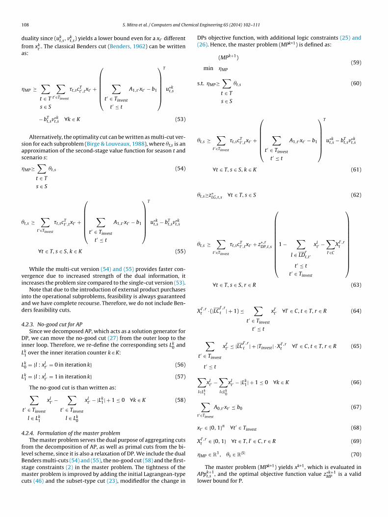
3. Bi-level decomposition algorithm

The bi-level decomposition algorithm tackles the original prob-lem (P) by alternately solving a relaxation and a restriction of P. Therelaxation of P, denoted as aggregated problem (AP), is built with asubset of the original primal constraints, based on domain-specificknowledge. The idea is that not all primal information is neededin order to determine good values for the complicating variablesof P. Once AP is solved, the complicating variables are restricted byeither fixing all of them to their respective values obtained from AP,or only fixing the variables that were found to be zero in AP. For therestricted complicating variables, the detailed problem (DP), which

is a restriction of P, is solved and primal cuts that are inferred from DPare added back to AP. The algorithm iterates until the gap betweenthe bounds obtained from AP and DP is within a predefined tol-erance. The generic bi-level decomposition algorithm is shown in

104 S. Mitra et al. / Computers and Chemical Engineering 65 (2014) 102–111

is a re

Frtf

ddrcitp

3

crwd

rabtttWnsoa

rvltttln

Fig. 1. Classical bi-level decomposition algorithm, in which AP

ig. 1. It was proved by Iyer and Grossmann (1998) that the algo-ithm converges within a finite number of iterations for the givenolerance, or enumerates in the worst case all feasible combinationsor the complicating variables.

The concept of complicating variables is the same as in Bendersecomposition (Benders, 1962; Geoffrion, 1972). However, Bendersecomposition tends to converge slowly if the underlying LP or NLPelaxation is weak (Sahinidis & Grossmann, 1991) since the dualuts are weak, as well as essential problem information is missingn the master problem. The bi-level decomposition algorithm aimso address this issue by incorporating some or most of the originalrimal constraints in its “master problem” (AP).

.1. Aggregated problem (AP)

It is important to recognize that there are multiple ways toonstruct AP. We identify several constraints that seem to be lesselevant in order to obtain a “good set” of investments for P, ofhich we discuss two options for subsets of constraints in moreetail.

The first option for a subset of constraints, which could beelaxed, contains the logic constraints (9)–(12) from Part I, whichre part of Yt,s. The logic constraints (9)–(12) restrict the transitionsetween operating modes and include minimum up- and down-imes and transitional times. If we relax these logic constraints,he number of second-stage variables is also reduced since theransitional variables ytr

t,s are no longer present in the problem.hile the number of constraints and variables is reduced sig-

ificantly, this relaxation has the drawback that it still containsecond-stage integer variables, and potentially underestimatesperating expenditures greatly since all costs related to transitionsre neglected.

The second option for a subset of constraints that could beelaxed, includes the integrality requirements for the second-stageariables for modes and transitions (ym

t,s and ytrt,s). While the prob-

em size is not reduced, the problem becomes considerably easiero solve since only a small number of integer variables, namely

he investment decisions xt′ , remain in the problem. Furthermore,ransitional costs are not entirely neglected. However, if the formu-ation were not tight in terms of the second-stage integer variables,either would be the relaxation.

laxation of the original problem (P) and DP is a restriction of P.

We notice that two conflicting objectives need to be balanced:the tightness of the relaxation (AP) and its difficulty to solve,which are both problem-dependent. Our computational experienceshows that the first option is faster to solve than the second option,despite the second-stage integer variables for operating modes. Onthe other hand, the relaxation of the second option is tighter sincetransitional cost is not entirely neglected.

However, an additional criterion could be to construct AP in away that AP yields a convex relaxation once the complicating vari-ables xt′ are fixed, which facilitates the application of additionaldecomposition methods to AP. From this perspective, the secondoption is more favorable. Interestingly, it corresponds to the con-vex relaxation suggested by Sundaramoorthy et al. (2012) for theircapacity planning problem in the pharmaceutical industry withinthe non-convex generalized Benders decomposition scheme. Whilewe pursue the second option, we note that the general frameworkof the bi-level decomposition algorithm provides additional toolsto speed up the solution process, such as primal cuts that will be dis-cussed later in this paper. Hence, AP is formulated in the followingway:

(AP) min∑

t′∈Tinvest

cTt′ xt′ +

∑t∈T,s∈S

�t,sdTt,syt,s (7)

s.t.∑

t′∈Tinvest

A0,t′ xt′ ≤ b0 (8)

∑t′∈Tinvest ,t′≤t

A1,t′ xt′ + B1yt,s ≤ b1 ∀t ∈ T, s ∈ S (9)

yt,s ∈ Yt,s ∀t ∈ T, s ∈ S (10)

xt′ ∈ {0, 1}n ∀t′ ∈ Tinvest (11)

where Yt,s is defined by relaxing the second-stage integrality con-straints for Yt,s:

Yt,s = {yt,s = (ymt,s, ytr

t,s, yct,s)

T, ym

t,s, ytrt,s, yc

t,s≥0 : Bt,syt,s ≤ bt,s} (12)

Additional cuts that augment (AP) and facilitate the solutionprocess will be described in Section 3.3.

emica

3

Gmftoadvtd

(

s

y

e

3

&h(diloo&cca

sitDoc

ss

3

(rc

Pros

Ptiars

S. Mitra et al. / Computers and Ch

.2. Detailed problem (DP)

Iyer and Grossmann (1998), as well as Erdirik-Dogan androssmann (2008), construct the detailed problem (DP) by aug-enting the original problem constraints with constraints on the

easible region of the complicating variables. More specifically, onlyhose complicating variables that correspond to zero in the solutionf AP are fixed. Therefore, all subsets for a given set of investmentsre evaluated implicitly in DP. However, in our case, the problemecouples in terms of seasons t and scenarios s only if all binaryariables for investments, xt′ , are fixed, which is denoted as xr

t′ (forhe rth iteration). Hence, we obtain the following definition for ouretailed problem (DPr):

DPr) min∑

t′∈Tinvest

cTt′ xr

t′ +∑

t∈T,s∈S

�t,sdTt,syt,s (13)

.t.∑

t′∈Tinvest ,t′≤t

A1,t′ xrt′ + B1yt,s ≤ b1 ∀t ∈ T, s ∈ S (14)

t,s ∈ Yt,s ∀t ∈ T, s ∈ S (15)

In practice, we can solve DPr individually for each season t andach scenario s.

.3. Cuts for AP

In the original work on bi-level decomposition (Erdirik-Dogan Grossmann, 2008; Iyer & Grossmann, 1998), three types of cutsave been proposed that can be added to the aggregated problemAP) for each iteration of the bi-level decomposition algorithm:esign cuts, superset cuts and subset cuts. The idea of design cuts

s to formulate valid bounds for major continuous variables, e.g.evels for capacity expansions, that become active once the previ-usly set of investments xr evaluated in DP is selected again (basedn a logic condition that is the same as the no-good cut by Balas

Jeroslow, 1972). Depending on the problem structure, supersetuts are formulated to exclude supersets of xr. Analogously, subsetuts exclude any subset of xr since DP is constructed in a way thatll subsets of xr are implicitly evaluated.

Unfortunately, we cannot directly apply any of these cuts. Super-et and subset cuts are not applicable since we cannot predict thempact of an investment in DP based on the solution in AP due tohe non-convexity of Yt,s. Furthermore, related to how we constructP, i.e. fixing all investment variables to their respective valuesbtained from AP to exploit the decomposable structure, the subsetuts would not be valid either.

However, in the following we describe subset-type cuts for theecond-stage value function that combine ideas from design andubset cuts, and do not cut off the optimal solution.

.3.1. Subset-type cuts for second-stage value functionThe idea of the subset-type cuts is to infer information on the

continuous) operating cost from DP for season t and scenario sather than excluding subsets from the feasible space of AP. Theuts are based on the following propositions:

roposition 3.1. Let z∗,rDP,t,s be the optimal objective value of the

ecourse function for season t and scenario s from DP for a given setf investments xr. Then, any subset of investments of xr will yield aecond-stage recourse function value of at least �t,sdT

t,syt,s≥z∗,rDP,t,s.

roof. All objective function cost coefficients are positive andhe coefficients in A1,t′ are such that the feasible region for yt,s is

ncreased if any xt′ is selected. Therefore, any subset of xr will have

more restricted feasible region for yt,s, compared to the feasibleegion for yt,s associated with xr. Hence, �t,sdT

t,syt,s≥z∗,rDP,t,s for any

ubset of xr. �

l Engineering 65 (2014) 102–111 105

Let us partition the set of investments N, in disjunctive invest-ments D, which are investments that can be executed only onceover the entire time horizon as by (2) (e.g. unique new equipmentor equipment upgrades), and cumulative investments C, whichare investments that can be executed multiple times (e.g. storagetanks), such that N = D ∪ C for any t′ ∈ Tinvest.

Proposition 3.2. If a given set of investments xr includes an elementl ∈ D, then the timing of the investment xl

t′ does not impact the boundon the second-stage value function for �t,sdT

t,syt,s from Proposition 3.1,

as long xlt′ is executed for t′ ≤ t.

Proof. In the linking constraint (3), which corresponds to con-straints (15) and (16) for equipment upgrades and constraints (18)and (19) for new equipment (Part I), the increase of the feasibleregion for yt,s is independent of the exact timing of the investmentxt′ , as long as t′ ≤ t. �

Proposition 3.3. For a given set of investments xr, the bound on�t,sdT

t,syt,s from Proposition 3.1 is invalid if an investment l ∈ C isselected at least one time more than in iteration r for t′ ≤ t.

Proof. For a given set of investments xr, the feasible region foryt,s increases further if an investment l ∈ C is executed one moretime for t′ ≤ t due to the linking constraint (3) (e.g. cumulativeincreases for inventory bounds in constraint (21) from Part I forstorage tanks). Therefore, �t,sdT

t,syt,s ≤ z∗,rDP,t,s, which concludes the

proof. �

Let us define the following sets, which partition the solution xr

for each iteration r according to whether investment l in time periodt′ in iteration r is a disjunctive or cumulative investment, and wasselected or not.

LDr0,t′ = {l : l ∈ D, xl

t′ = 0 in iteration r} (16)

LDr1,t′ = {l : l ∈ D, xl

t′ = 1 in iteration r} (17)

LCr0,t′ = {l : l ∈ C, xl

t′ = 0 in iteration r} (18)

LCr1,t′ = {l : l ∈ C, xl

t′ = 1 in iteration r} (19)

Furthermore, we introduce as follows the set LDrt,t′ , which indi-

cates whether a disjunctive investment has not been executedbefore season t:

LDrt,t′ =

⎧⎪⎪⎪⎪⎪⎨⎪⎪⎪⎪⎪⎩

l : l ∈ LDr0,t′ , l /∈

⋃

t′′ ∈ Tinvest

t′′ ≤ t

LDr1,t′′

⎫⎪⎪⎪⎪⎪⎬⎪⎪⎪⎪⎪⎭

∀t ∈ T, t′ ∈ Tinvest, t′ ≤ t, r ∈ R (20)

The set LCl,rt indicates how often the cumulative investment l ∈ C

has been selected for t′ ≤ t in iteration r:

LCl′,rt =

⋃

t′ ∈ Tinvest

LCl′,r1,t′ ∀l′ ∈ C, t ∈ T, r ∈ R (21)

t′ ≤ t

Based on Propositions 3.1–3.3, we can formulate the follow-ing logic statement, for which, if it is true, the bound on the

1 emica

si

utt

�

X

t

⇒

⇐

tit

3

sb1

t

L

L

06 S. Mitra et al. / Computers and Ch

econd-stage value function for season t and scenario s becomesnvalid (Xl′,r

t is defined further below):∨

l ∈ LDrt,t′

t′ ≤ t

t′ ∈ Tinvest

xlt′∨l′∈C

Xl′,rt ∀t ∈ T, s ∈ S, r ∈ R (22)

We can translate the logic statement (22) into the following cutssing propositional logic (Raman & Grossmann, 1993), assuminghat the bound obtained from the previous iteration r is valid unlesshe logic statement becomes true:

t,sdTt,syt,s≥z∗,r

DP,t,s

⎛⎜⎜⎜⎜⎜⎜⎜⎜⎜⎜⎝

1 −∑

l ∈ LDrt,t′

t′ ≤ t

t′ ∈ Tinvest

xlt′ −

∑l′∈C

Xl′,rt

⎞⎟⎟⎟⎟⎟⎟⎟⎟⎟⎟⎠

∀t ∈ T, s ∈ S, r ∈ R (23)

In Eqs. (22) and (23), Xl′,rt is defined as follows:

l′,rt = 1 ⇔ Investment l′ ∈ C is selected more than (24)

|LCl′,rt | times for t′ ≤ t, t′ ∈ Tinvest in iteration r

To establish this link between xl′t′ and Xl′,r

t , we need to formulatehe following two logic relationships:

: Xl′,rt · (|LC

l′,rt | + 1) ≤

∑

t′ ∈ Tinvest

t′ ≤ t

xl′t′ ∀l′ ∈ C, t ∈ T, r ∈ R (25)

:∑

t′ ∈ Tinvest

t′ ≤ t

xl′t′ ≤ |LC

l′,rt | + |Tinvest | · Xl′,r

t ∀l′ ∈ C, t ∈ T, r ∈ R (26)

In summary, Eqs. (23), (25) and (26) need to be included in APo establish the subset-type cut based on previous DP solutions. Ast will be shown in the results, these cuts can have a big impact inerms of a reduction of computational time.

.3.2. No-good cutOnce a given set of investments xr has been evaluated in DP, the

ame set should not be visited again in AP, which can be enforcedy formulating the following no-good/integer cut (Balas & Jeroslow,972):

∑

t′ ∈ Tinvest

l ∈ Lr1

xlt′ −

∑

t′ ∈ Tinvest

l ∈ Lr0

xlt′ − |Lr

1| + 1 ≤ 0 ∀r ∈ R (27)

In (27), Lr0 and Lr

1 are defined as follows (independent whetherhe investment is disjunctive or cumulative):

r0 = {l : xl

t′ = 0 in iteration r} (28)

r1 = {l : xl

t′ = 1 in iteration r} (29)

l Engineering 65 (2014) 102–111

3.4. Discussion of scalability of the classical bi-leveldecomposition algorithm

While each operational subproblem (DP), (13)–(15), is an MILPthat represents the detailed weekly schedule on an hourly basis, thesolution process of DP scales well in the sense that it can poten-tially be parallelized since each operational problem for season tand scenario s can be solved individually. In contrast, the size of AP,(7)–(11), and its associated solution time depends on the numberof individual operational subproblems. For a large set of seasonsand scenarios, AP will still be hard to solve. Therefore, we needadditional algorithmic techniques to enable the solution of AP in ascalable manner.

4. Ingredients for an enhanced bi-level decompositionalgorithm

In the following, we describe the ingredients for a decompo-sition algorithm that is based on the previously outlined bi-levelscheme. First, we revisit the detailed problem (DP), and introducea modification in the objective function that allows us to deriveadditional Lagrangean-type cuts that can be included in AP dur-ing the initialization phase to improve the tightness of AP. Second,the application of Benders decomposition to AP is discussed, whichfacilitates the solution of AP independent of the number of seasonsand scenarios.

4.1. Detailed problem (DP)

To enable the Lagrangean-type cuts, we reformulate the detailedproblem (DP), which is defined by Eqs. (13)–(15), by distributing thefirst-stage investment cost of (13) over all scenarios, in the spirit ofthe scenario decomposition approach (Caroe & Schultz, 1999). Forthis purpose we split the cost coefficients as follows: ct′ =

∑t∈T ct′,t .

The detailed problem can be written as:

(DPr) min∑

t∈T,s∈S

∑t′∈Tinvest

�t,scTt′,tx

rt′ +

∑t∈T,s∈S

�t,sdTt,syt,s (30)

s.t.∑

t′∈Tinvest ,t′≤t

A1,t′ xrt′ + B1yt,s ≤ b1 ∀t ∈ T, s ∈ S (31)

yt,s ∈ Yt,s ∀t ∈ T, s ∈ S (32)

4.1.1. Detailed subproblems for each season and scenarioIn practice, we solve DP for each season t and scenario s inde-

pendently, for which we define (DPrt,s) as:

(DPrt,s) min

∑t′∈Tinvest

�t,scTt′,tx

rt′ + �t,sd

Tt,syt,s (33)

s.t.∑

t′∈Tinvest ,t′≤t

A1,t′ xrt′ + B1yt,s ≤ b1 (34)

yt,s ∈ Yt,s (35)

Let z∗rDP,t,s be the optimal solution of DPr

t,s. Then, the optimal solu-tion of the rth iteration of DP, z∗r

DP , is defined as z∗rDP =

∑t∈T,s∈Sz∗r

DP,t,s.

4.1.2. Initial Lagrangean-type cutsThe solution of the non-convex problem (DP) is a time-

consuming ingredient of our algorithm, and we would like tominimize the number of DP evaluations. As described previously,

the reformulation of the objective function as per (30) allows us tosolve a Lagrangean-type reformulation of DP, denoted as LG, duringthe initialization phase to find strong initial bounds. The idea is toduplicate the first-stage investment variables xt′ for each season t

emica

avaca

(

s

t

y

x

s

(

s

t

y

x

Ls

t

towi

4

aaasscot

poGTiA

lt

S. Mitra et al. / Computers and Ch

nd scenario s, denoted as xt′,t,s, and solve each subproblem indi-idually such that the same investment decisions are not enforcedcross all scenarios. We obtain the formulation (LG), which is a non-onvex relaxation of DP and is expected to yield good initial boundss follows:

LG) min∑

t∈T,s∈S

∑t′∈Tinvest

�t,scTt′,txt′,t,s +

∑t∈T,s∈S

�t,sdTt,syt,s (36)

.t.∑

t′∈Tinvest

A0,t′ xt′,t,s ≤ b0 ∀t ∈ T, s ∈ S (37)

∑′∈Tinvest ,t′≤t

A1,t′ xt′,t,s + B1yt,s ≤ b1 ∀t ∈ T, s ∈ S (38)

t,s ∈ Yt,s ∀t ∈ T, s ∈ S (39)

t′,t,s ∈{

0, 1}n ∀t′ ∈ Tinvest, t ∈ T, s ∈ S (40)

LG can be decomposed and formulated for each season t andcenario s as (LGt,s):

LGt,s) min∑

t′∈Tinvest

�t,scTt′,txt′,t,s + �t,sd

Tt,syt,s (41)

.t.∑

t′∈Tinvest

A0,t′ xt′,t,s ≤ b0 (42)

∑′∈Tinvest ,t′≤t

A1,t′ xt′,t,s + B1yt,s ≤ b1 (43)

t,s ∈ Yt,s (44)

t′,t,s ∈ {0, 1}n ∀t′ ∈ Tinvest (45)

Let z∗LG,t,s =

∑t′∈Tinvest

�t,scTt′,tx

∗t′,t,s + �t,sdT

t,sy∗t,s be the solution of

Gt,s. Note that z∗LG,t,s yields a valid lower bound for the cost in

eason t and scenarios s in DPt,s:∑′∈Tinvest

�t,scTt′,txt′ + �t,sd

Tt,syt,s≥z∗

LG,t,s ∀t ∈ T, s ∈ S (46)

Remark: From a Lagrangean relaxation perspective, we relaxhe non-anticipativity constraints for xt′,t,s, which enforce equalityf xt′,t,s across all scenarios, and solve the Lagrangean relaxationith the Lagrangean multipliers set to zero once during the initial-

zation phase.

.2. Decomposition of AP

The bottleneck of the classical bi-level decomposition is theggregated problem (AP), which grows as the number of seasonsnd scenarios increases. Interestingly, AP has only a few binary vari-bles, the first-stage investment decisions, which complicate theolution of the problem. If we fix the first-stage investment deci-ions, AP decouples into individual subproblems, which only haveontinuous variables and are linear. For this setup, the applicationf Benders decomposition to AP is a natural one that we discuss inhe following.

Note that AP could also be decomposed with Lagrangean decom-osition, which would lead to a hybrid scheme similar to thenes described by Calfa et al. (2013) and Terrazas-Moreno androssmann (2011). However, both report dual gaps. Furthermore,errazas-Moreno and Grossmann (2011) remove the upper bound-ng procedure of AP, which potentially weakens the strength of the

P bound.

In general, the application of Lagrangean decomposition canead to the presence of a duality gap, which requires fur-her branch and bound search. Furthermore, the update of the

l Engineering 65 (2014) 102–111 107

Lagrangean multipliers, as well as the application of a heuris-tic to find first-stage feasible solutions, is known to be difficultfor Lagrangean decomposition. Additionally, the addition of inte-ger cuts like the ones described in Section 3.3 to the Lagrangeandual requires the application of a somewhat complicated re-optimization scheme (Frangioni, 2005) if cutting planes are usedto update the Lagrangean multipliers.

4.2.1. Benders subproblems for APWe apply Benders decomposition for AP, which decouples into

subproblems for each season t and scenario s. Note that we needto modify the objective function according to the change in DPsobjective function (33). We formulate the Benders subproblem inits primal form as follows for a given set of investments xk

t′ , wherek ∈ K is the counter of the inner loop for the decomposition of AP:

(APpkt,s) min

∑t′∈Tinvest

�t,scTt′,tx

kt′ + �t,sd

Tt,syt,s (47)

s.t. B1yt,s ≤ b1 −∑

t′ ∈ Tinvest

t′ ≤ t

A1,t′ xkt′ (48)

yt,s ∈ Yt,s (49)

Let ut,s be the dual multiplier associated with constraint (48)and vt,s be the dual multiplier of constraint (49), which representsBt,syt,s ≤ bt,s according to the definition of Yt,s in (12). Then, the dualof APpt,s can be written as:

(APdkt,s) max

∑t′∈Tinvest

�t,scTt′,tx

kt′ +

⎛⎜⎜⎜⎜⎜⎝

∑

t′ ∈ Tinvest

t′ ≤ t

A1,t′ xkt′ − b1

⎞⎟⎟⎟⎟⎟⎠

T

ut,s

− bTt,svt,s (50)

s.t. − uTt,sB1 − vT

t,sBt,s ≤ �t,sdt,s (51)

ut,s, vt,s≥0 (52)

Let y∗kt,s be the solution of APpk

t,s and (u∗kt,s, v∗k

t,s) be the solution of

APdkt,s. Let us define z∗k

AP,t,s, in the following way (equivalence dueto strong duality):

z∗kAP,t,s =

∑t′∈Tinvest

�t,scTt′,tx

kt′ + �t,sd

Tt,sy

∗kt,s

=∑

t′∈Tinvest

�t,scTt′,tx

kt′ +

⎛⎜⎜⎜⎜⎜⎝

∑

t′ ∈ Tinvest

t′ ≤ t

A1,t′ xkt′ − b1

⎞⎟⎟⎟⎟⎟⎠

T

u∗kt,s − bT

t,sv∗kt,s

The optimal solution of the kth iteration of AP, z∗kAP , is therefore

defined as z∗kAP =

∑t∈T,s∈Sz∗k

AP,t,s.

4.2.2. Dual Benders optimality cutsWith the dual solution (u∗k

t,s, v∗kt,s) from APpk

t,s, we can derive Ben-ders optimality cuts for AP. The Benders cuts are based on weak

1 emica

d

fa

�

sas

�

�

vi

iad

4

DiL

L

L

4

flBsmc

08 S. Mitra et al. / Computers and Ch

uality since (ukt,s, vk

t,s) yields a lower bound even for a xt′ different

rom xkt′ . The classical Benders cut (Benders, 1962) can be written

s:

MP ≥∑

t ∈ T

s ∈ S

∑t′∈Tinvest

�t,scTt′,txt′ +

⎛⎜⎜⎜⎜⎜⎝

∑

t′ ∈ Tinvest

t′ ≤ t

A1,t′ xt′ − b1

⎞⎟⎟⎟⎟⎟⎠

T

u∗kt,s

− bTt,sv

∗kt,s ∀k ∈ K (53)

Alternatively, the optimality cut can be written as multi-cut ver-ion for each subproblem (Birge & Louveaux, 1988), where �t,s is anpproximation of the second-stage value function for season t andcenario s:

MP≥∑

t ∈ T

s ∈ S

�t,s (54)

t,s ≥∑

t′∈Tinvest

�t,scTt′,txt′ +

⎛⎜⎜⎜⎜⎜⎝

∑

t′ ∈ Tinvest

t′ ≤ t

A1,t′ xt′ − b1

⎞⎟⎟⎟⎟⎟⎠

T

u∗kt,s − bT

t,sv∗kt,s

∀t ∈ T, s ∈ S, k ∈ K (55)

While the multi-cut version (54) and (55) provides faster con-ergence due to increased strength of the dual information, itncreases the problem size compared to the single-cut version (53).

Note that due to the introduction of external product purchasesnto the operational subproblems, feasibility is always guaranteednd we have complete recourse. Therefore, we do not include Ben-ers feasibility cuts.

.2.3. No-good cut for APSince we decomposed AP, which acts as a solution generator for

P, we can move the no-good cut (27) from the outer loop to thenner loop. Therefore, we re-define the corresponding sets Lk

0 andk1 over the inner iteration counter k ∈ K:

k0 = {l : xl

t′ = 0 in iteration k} (56)

k1 = {l : xl

t′ = 1 in iteration k} (57)

The no-good cut is than written as:∑

t′ ∈ Tinvest

l ∈ Lk1

xlt′ −

∑

t′ ∈ Tinvest

l ∈ Lk0

xlt′ − |Lk

1| + 1 ≤ 0 ∀k ∈ K (58)

.2.4. Formulation of the master problemThe master problem serves the dual purpose of aggregating cuts

rom the decomposition of AP, as well as primal cuts from the bi-

evel scheme, since it is also a relaxation of DP. We include the dualenders multi-cuts (54) and (55), the no-good cut (58) and the first-tage constraints (2) in the master problem. The tightness of theaster problem is improved by adding the initial Lagrangean-type

uts (46) and the subset-type cut (23), modifiedfor the change in

l Engineering 65 (2014) 102–111

DPs objective function, with additional logic constraints (25) and(26). Hence, the master problem (MPk+1) is defined as:

(MPk+1)

min �MP

(59)

s.t. �MP≥∑

t ∈ T

s ∈ S

�t,s (60)

�t,s ≥∑

t′∈Tinvest

�t,scTt′,txt′ +

⎛⎜⎜⎜⎜⎜⎝

∑

t′ ∈ Tinvest

t′ ≤ t

A1,t′ xt′ − b1

⎞⎟⎟⎟⎟⎟⎠

T

u∗kt,s − bT

t,sv∗kt,s

∀t ∈ T, s ∈ S, k ∈ K (61)

�t,s≥z∗LG,t,s ∀t ∈ T, s ∈ S (62)

�t,s ≥∑

t′∈Tinvest

�t,scTt′,txt′ + z∗,r

DP,t,s

⎛⎜⎜⎜⎜⎜⎜⎜⎜⎜⎜⎜⎝

1 −∑

l ∈ LDrt,t′

t′ ≤ t

t′ ∈ Tinvest

xlt′ −

∑l′∈C

Xl′,rt

⎞⎟⎟⎟⎟⎟⎟⎟⎟⎟⎟⎟⎠

∀t ∈ T, s ∈ S, r ∈ R (63)

Xl′,rt · (|LC

l′,rt | + 1) ≤

∑

t′ ∈ Tinvest

t′ ≤ t

xl′t′ ∀l′ ∈ C, t ∈ T, r ∈ R (64)

∑

t′ ∈ Tinvest

t′ ≤ t

xl′t′ ≤ |LC

l′,rt | + |Tinvest | · Xl′,r

t ∀l′ ∈ C, t ∈ T, r ∈ R (65)

∑l∈Lk

1

xlt′ −

∑l∈Lk

0

xlt′ − |Lk

1| + 1 ≤ 0 ∀k ∈ K (66)

∑t′∈Tinvest

A0,t′ xt′ ≤ b0 (67)

xt′ ∈ {0, 1}n ∀t′ ∈ Tinvest (68)

Xl′,rt ∈ {0, 1} ∀t ∈ T, l′ ∈ C, r ∈ R (69)

�MP ∈ R1, �s ∈ R

|S| (70)

The master problem (MPk+1) yields xk+1, which is evaluated inAPpk+1

t,s , and the optimal objective function value z∗k+1MP is a valid

lower bound for P.

S. Mitra et al. / Computers and Chemical Engineering 65 (2014) 102–111 109

thin a

5

5

d1

2

3

4

5

6

7

5

di

Fig. 2. Algorithmic flow (bold arrows) and flow of information (

. The enhanced hybrid bi-level decomposition algorithm

.1. Algorithm EBL-multi + LG + subset

In the following we describe the enhanced hybrid bi-levelecomposition algorithm, which is depicted in Fig. 2.. Initialization of algorithm

Set k = 1, K = {}, K′ = {}, r = 1, R = {}, xk=1 = 0,LB =− ∞, UBAP =∞, UB =∞, tol ≥ 0,Go to step 2

. Initial Lagrangean-type cuts from LGSolve LGt,s , (41)–(45), ∀t ∈ T, s ∈ S in parallel and store z∗

LG,t,s

Go to step 3

. Benders subproblems of APFor given xk , solve APpk

t,s , (47)–(49), ∀t ∈ T, s ∈ S in parallelStore dual multipliers u*k , v∗k and generate sets Lk

0, Lk1, K = K ∪ {k}

If z∗kAP

< UBAP : UBAP = z∗kAP

and xr = xk , k′ = kGo to step 4

. Master problem (MP)

For given u*k , v∗k , Lk0, Lk

1, z∗LG,t,s

, z∗,rDP,t,s

, LDr

t,t′ , LCl,r

t :Solve (MPk+1), (59)–(70), and store solution as xk+1

If z∗k+1MP

> LB: LB = z∗k+1MP

Go to step 5

. Convergence check for inner loopIf UBAP − LB ≤ 0 or UB − LB ≤ tol: Go to step 6Else: Set k = k + 1, go to step 3

. Detailed problem (DP)If UB − UBAP > tol:

For given xr , solve DPrt,s , (33)–(35), ∀t ∈ T, s ∈ S in parallel

R = R ∪ {r}, K′ = K′ ∪ {k′}If z∗k

DP< UB: UB = z∗k

DP, solution = (xr , y∗

t,s)DPIf K\ K′ = ∅: UBAP =∞Else: k′ = argmink∈K\K ′ {z∗k

AP}, UBAP = z∗k′

AP, xr = xk′

Go to step 7

. Convergence check for outer loopIf UB − UBAP ≤ tol and UB − LB ≤ tol: Stop and return solutionElse: Set r = r + 1, go to step 5

.2. Further variants of the algorithm

In this section, we define “reduced” variants of the previouslyescribed algorithm EBL-multi + LG + subset in order to test the

mpact of the individual components of the algorithm.

rrows) for our enhanced hybrid bi-level decomposition scheme.

5.2.1. EBL-singleIn the first variant, we remove the Lagrangean-type cuts (step

2) completely, and do not use the subset type cuts, Eqs. (63)–(65),in the master problem. Furthermore, we use the classical Benderscut, Eq. (53), in place of the multi-cut (60) and (61).

Remark: The bi-level decomposition algorithm with classicalBenders single cuts for (AP), denoted by EBL-single, is equiva-lent to non-convex generalized Benders decomposition appliedto two-stage stochastic programming problem, as described bySundaramoorthy et al. (2012) for a capacity planning problem inthe pharmaceutical industry.

5.2.2. EBL-multiIn this variant, we remove the Lagrangean-type cuts (step 2)

completely, and do not use the subset type cuts, Eqs. (63)–(65), inthe master problem. The rest of the algorithm is as described inSection 5.1.

5.2.3. EBL-multi + LGThe only difference between EBL-multi + LG and the algorithm

we described in Section 5.1 is that we do not use the subset-typecuts, Eqs. (63)–(65), in the master problem.

5.3. Convergence of the algorithm

A formal proof of convergence for the bi-level decompositionalgorithm was given by Iyer and Grossmann (1998), and a prooffor the non-convex generalized Benders decomposition was statedby Barton and co-workers (Li et al., 2011; Sundaramoorthy et al.,2012). Therefore, we omit the proof in this paper.

Furthermore, we would like to comment on the issue of thetightness of the relaxation (AP). If the relaxation of AP is weak, wemight enumerate all investments and observe a slow progress inthe lower bound obtained from the master problem. The additionof the Lagrangean-type cuts from (LG) and the subset-type cuts ismotivated by this potential issue.

6. Computational aspects

6.1. Parallel implementation

The Lagrangean-type relaxation (LGt,s), the Benders subprob-lems for APpk

t,s and the detailed problem (DPrt,s) can be decomposed

110 S. Mitra et al. / Computers and Chemical Engineering 65 (2014) 102–111

Table 1Sizes of the resulting optimization problems. Except for MP, which depends on the number of iterations, the sizes are the same for all problem instances (1–4). Note that thenumbers for MP correspond to case 3 for the EBL-multi + LG + subset scheme.

Full-space DPrt,s LGt,s APk

t,s MP MPk = 1, r = 1 k = 14, r = 6

Number of op. problems 60 1 1 1 – –Constraints 915,270 14,958 14,958 14,958 184 1877

39,840 39,840 141 4413716 0 20 320

20 0 20 20

ittpolaml

6

dnomC&mscs

llcls

totivt

1

2

3

4

6

tbf

Fig. 3. Convergence of the inner iteration in case 2: scaled lower bound from MP.

Variables 2,388,984 39,840

Binary Var. 221,780 3696

Binary Invest. 20 0

nto operational subproblems for each season t and scenario s. Notehat these subproblems can be solved in parallel. Hence, we usehe GAMS grid computing environment (Bussieck et al., 2009) toarallelize the solution process for LGt,s, APpk

t,s and DPrt,s. We run

ur implementation on a machine with 8 cores, which were uti-ized in the parallelization. The same code could be executed on

‘real’ grid computing environment, in which we envision that auch larger number of scenarios could be easily solved in paral-

el.

.2. Discussion of case study setup

We solve the same test cases (cases 1–4 for varying baselineemand, growth rate, demand distribution and prices for exter-al product purchases) that were reported in Part I of the papern the same computing machine, an Intel i7-2600 (3.40 GHz)achine with 8 processors and 8 GB RAM. The commercial solver

PLEX 12.4.0.1 was employed in GAMS 23.9.1 (Brooke, Kendrick, Meeraus, 2012). The termination criterion was set to 0.5% opti-ality gap. Note that the algorithm could accept and converge for

maller values as well, but we choose 0.5% to make our numbersomparable with the full-space approach, in which we allowed theame final gap.

As we can see in Table 1, the resulting full-space model is veryarge, as it has almost 1 million constraints and more than 2 mil-ion variables, of which there are more than 200,000 binaries. Inontrast, we can observe that the problem sizes for each subprob-em for one season and scenario in DPr

t,s, LGt,s and APkt,s are (not

urprisingly) much smaller.We compare the full-space solution (as reported in Part I of

he paper for which we used the parallel computing capabilitiesf CPLEX by setting threads=8) with four different variants ofhe decomposition algorithm, and investigate the impact of eachndividual component in the decomposition algorithm. The fourariants are described in detail in Section 5, and we shortly restatehem here:

. EBL-single: Hybrid bi-level decomposition with single cut Ben-ders decomposition for (AP)

. EBL-multi: Hybrid bi-level decomposition with multi-cut Ben-ders decomposition for (AP)

. EBL-multi + LG: Hybrid bi-level decomposition with multi-cutBenders decomposition for AP and the initial Lagrangean-typecuts from LG

. EBL-multi + LG + subset: Hybrid bi-level decomposition withmulti-cut Benders decomposition for AP, the initial Lagrangean-type cuts from LG and the subset-type cuts from DP, i.e. like thealgorithm we described in Section 5.

.3. Discussion of results

Due to confidentiality issues, we cannot disclose the final objec-ive function values. However, we can confirm that all hybridi-level decomposition schemes converge to the same final solutionor each case. Furthermore, the same investments are proposed in

Fig. 4. Convergence of the outer iteration in case 2: scaled upper bound from DP.

the full-space method and in each of the hybrid bi-level decompo-sition schemes. Thus, we can conclude that the full-space method’smajor issue is to prove optimality due to the large number of binaryvariables.

We illustrate the convergence of the different versions of thealgorithm for case 2. We report the convergence progress of theoverall lower bound obtained from the master problem (MP) in theinner iteration in Fig. 3, and the overall upper bound from DP inthe outer iteration in Fig. 4. One can clearly observe the impact ofthe cuts in terms of a strengthened relaxation for the lower boundand a reduced number of inner iterations. When subset cuts areapplied, the number of outer iterations is also reduced.

We report the total execution times in seconds, and the numberof AP and DP evaluations in Table 2. The most time-consuming partof the algorithm is the detailed problem (DP), which is a detailedscheduling problem (MILP) for an entire week on an hourly foreach season t and scenario s. In fact, DP can consume 90% or moreof the total execution time since one (AP) evaluation takes only40–50 s. Therefore, the impact on execution time of the multi cutsin EBL-multi is small compared to EBL-single since it only reducesthe number of AP evaluations. In contrast, the Lagrangean-typecuts from LG reduce the number of DP iterations in the diffi-cult cases 3 and 4, and saves 20–25% in computational time. Theaddition of the subset-type cuts (EBL-multi + LG + subset) has thelargest impact on computational time since we can observe another50–80% reduction compared to EBL-multi + LG and a speed-up of

45–85% compared to the EBL-single scheme. If we compare thetimes for our most advanced scheme (EBL-multi + LG + subset) withthe full space method we can observe a speed-up of up to two ordersof magnitude across all four test cases.

S. Mitra et al. / Computers and Chemica

Table 2Comparison of computational times for the full-space method and the differentvariants of the hybrid bi-level decomposition algorithm. Allowed gap in full-space:0.50%.

Method Property Case 1 Case 2 Case 3 Case 4

Full-space Time (s) 78,810 67,137 288,000 154,312Full-space Gap 1.32%a 0.50% 3.23%b 0.60%a

All EBL-schemes Gap <0.50% <0.50% <0.50% <0.50%

EBL-single Time (s) 721 4321 9832 16,345EBL-single AP 14 28 43 33EBL-single DP 1 5 16 14

EBL-multi Time (s) 583 3820 9097 16,009EBL-multi AP 11 18 28 24EBL-multi DP 1 5 16 14

EBL-multi + LG Time (s) 403 3930 6415 11,925EBL-multi + LG AP 1 13 21 17EBL-multi + LG DP 1 5 14 11

EBL-multi + LG + subset Time (s) 403 1869 2846 2436EBL-multi + LG + subset AP 1 9 14 9EBL-multi + LG + subset DP 1 2 7 3

In bold, the longest and shortest CPU times are highlighted.

7

bttsdtfgasltoaf

A

F

a Out of memory.b Terminated after 80 h of computation.

. Conclusion

In this paper (Part II), we have described an enhanced hybridi-level decomposition scheme that combines bi-level decomposi-ion with Benders decomposition and additional cuts to strengthenhe relaxation. We have solved a set of instances for a large multi-cale capacity planning problem based on industrial data with theecomposition scheme, and we were able to reduce the compu-ational time by up to two orders of magnitude compared to theull-space method and by 45–85% compared to a pure non-convexeneralized Benders approach. The results were obtained due todditional cuts obtained from a Lagrangean-type relaxation andubset-type cuts from the detailed problem (DP) that exploit theinking structure between investment and operational variables inhe problem. For future work, it would be interesting to explorether cuts from the structure of DP or other (non-convex) relax-tions of DP that can be utilized to yield strong bounds in order tourther reduce the number of DP evaluations.

cknowledgments

We would like to thank Praxair, Inc., and the National Scienceoundation for financial support under grant CBET-1159443.

l Engineering 65 (2014) 102–111 111

References

Balas, E., & Jeroslow, R. G. (1972). Canonical cuts on the unit hypercube. SIAM Journalof Applied Mathematics, 23, 61–69.

Benders, J. F. (1962). Partitioning procedures for solving mixed-variables program-ming problems. Numerische Mathematik, 4, 238–252.

Birge, J. R., & Louveaux, F. (2011). Introduction to stochastic programming. Springerseries in operations research. New York: Springer.

Birge, J. R., & Louveaux, F. V. (1988). A multicut algorithm for two-stage stochasticlinear programs. European Journal of Operational Research, 34, 384–392.

Brooke, A., Kendrick, D., & Meeraus, A. (2012). GAMS: A users guide, Release 23.9.1.South San Francisco: The Scientific Press.

Bussieck, M. R., Ferris, M. C., & Meeraus, A. (2009). Grid-enabled optimization withGAMS. INFORMS Journal on Computing, 21, 349–362.

Calfa, B. A., Agarwal, A., Grossmann, I. E., & Wassick, J. M. (2013). Hybridbilevel-Lagrangean decomposition scheme for the integration of planning andscheduling of a network of batch plants. Industrial & Engineering ChemistryResearch, 52, 2152–2167.

Caroe, C. C., & Schultz, R. (1999). Dual decomposition in stochastic integer program-ming. Operations Research Letters, 24, 37–45.

Erdirik-Dogan, M., & Grossmann, I. E. (2008). Simultaneous planning and schedulingof single-stage multi-product continuous plants with parallel lines. Computers& Chemical Engineering, 32, 2664–2683.

Frangioni, A. (2005). About Langrangian methods in integer optimization. Annals ofOperations Research, 139, 163–193.

Geoffrion, A. M. (1972). Generalized benders decomposition. Journal of OptimizationTheory and Applications, 10, 237–260.

Guignard, M. (2003). Lagrangean relaxation. Top, 11, 151–228.Guignard, M., & Kim, S. (1987). Lagrangean decomposition – A model yielding

stronger Lagrangean bounds. Mathematical Programming, 39, 215–228.Iyer, R., & Grossmann, I. E. (1998). A bilevel decomposition algorithm for long-range

planning of process networks. Industrial & Engineering Chemistry Research, 37,474.

Karuppiah, R., & Grossmann, I. E. (2008). A Lagrangean based branch-and-cut algo-rithm for global optimization of nonconvex mixed-integer nonlinear programswith decomposable structures. Journal of Global Optimization, 41, 163–186.

Li, X., Tomasgard, A., & Barton, P. I. (2011). Nonconvex generalized benders decom-position for stochastic separable mixed-integer nonlinear programs. Journal ofOptimization Theory and Applications, 151, 425–454.

Raman, R., & Grossmann, I. E. (1993). Modeling and computational techniquesfor logic based integer programming. Computers & Chemical Engineering,18, 563.

Sahinidis, N. V., & Grossmann, I. E. (1991). Convergence properties of generalizedbenders decomposition. Computers & Chemical Engineering, 15, 481–491.

Sundaramoorthy, A., Li, X., Evans, J. M. B., & Barton, P. I. (2012). Capacity planningunder clinical trials uncertainty in continuous pharmaceutical manufactur-ing, 2: Solution method. Industrial & Engineering Chemistry Research, 51,13703–13711.

Terrazas-Moreno, S., & Grossmann, I. E. (2011). A multiscale decomposi-tion method for the optimal planning and scheduling of multi-sitecontinuous multiproduct plants. Chemical Engineering Science, 66,4307–4318.

van den Heever, S. A., & Grossmann, I. E. (1999). Disjunctive multiperiod optimizationmethods for design and planning of chemical process systems. Computers &Chemical Engineering, 23, 1075.

Van Slyke, R., & Wets, R. J. B. (1969). L-shaped linear programs with applicationsto optimal control and stochastic programming. SIAM Journal on Applied Mathe-

matics, 17, 638–663.

You, F., Grossmann, I. E., & Wassick, J. M. (2011). Multisite capacity, production anddistribution planning with reactor modifications: MILP model, bilevel decompo-sition algorithm vs. Lagrangean decomposition scheme. Industrial & EngineeringChemistry Research, 50, 4831–4849.