optimal low earth orbit transfers with drag sails
TRANSCRIPT

Politecnico di Torino
Master's Degree in Aerospace Engineering
Master's Thesis
Optimal low Earth orbit transfers with drag sails
Supervisor: Prof. Lorenzo Casalino
Co-Supervisor: Prof. Francesco Topputo
Author:
Andrea Forestieri
April 2021

A Pippo,
ovunque tu sia ora, spero che sia ruscito a trovare la serenità che tanto meriti,
amico mio.

Acknowledgments
Ringrazio di cuore il Prof. Casalino e il Prof. Topputo, per avermi dato l'opportunità
di sviluppare un argomento di mio grande interesse.
Un sentito ringraziamento anche al Dott. Fasano, per i suoi preziosi consigli e
per tutte le opportunità che mi ha dato.
Ai miei genitori: grazie per aver sempre avuto ducia nelle mie capacità, per aver
sempre investito su di me, per avermi lasciato libero di seguire le mie ambizioni, per
aver sempre fatto di tutto anché io non perdessi nessuna opportunità che mi si
presentava davanti e, prima di tutto, per essere sempre stati dei modelli da seguire.
A mio fratello Giacomo: per te niente frasi strappalacrime. In fondo, io e te siam
tipi coincisi. Sappi solo che, nonostante tutte le azzuate, ti ringrazio per essere un
fratello generoso ed è bello sapere di avere le proprie spalle coperte.
Desidero inoltre ringraziare Mattia e Vittoria, con cui ho condiviso tanto in questo
percorso ed ancor prima di esso. Grazie per esserci sempre stati e per avermi aiutato
quando ne avevo più bisogno. Avervi come amici è un privilegio.
Ringrazio inoltre tutta la compagnia de gli Olbicelli. Un ringraziamento sentito
a Fra, per essere stato un fratello maggiore e l'artece di tutte le avventure più pazze
che ho vissuto in questi anni. Lalla e Loris, da quando vi ho conosciuto ci avete
messo poco a diventare delle persone importanti. Grazie per essermi stati accanto,
soprattutto nell'ultimo dicile periodo. A Manu, per tutte le discussioni losoche
davanti alle tante, forse troppe, birre del MacGilly's. Ad Andre e Vale, per la vostra
gentilezza e per avere portato un po' di vivacità nel freddo di Torino.
Come non ringraziare anche tutti i miei colleghi di corso per tutte le giornate
passate tra i corridoi del Poli, per i pranzi insieme, per le chiacchiere scambiate in
la alle macchinette del caè, per le ore passate a ripetere e per quelle passate a far
festa. Senza di voi non sarebbe stata la stessa esperienza.
E grazie a te, Chiara, che riesci sempre a tirare fuori il meglio di me. Senza di
te, la redazione di questa tesi sarebbe stata immensamente più dicoltosa. Grazie
per essere la mia voce quando non sono abbastanza forte per parlare e per rendermi
ogni giorno un uomo migliore.
Grazie.

Abstract
Satellite operations in low Earth orbit will be extremely frequent in the near fu-
ture, and consequently the optimization of trajectories between such orbits is becom-
ing of extreme interest. Low-thrust electric propulsion will arguably be the preferred
option for many missions, as it provides benets in terms of propellant consump-
tion. Low-thrust trajectories in low Earth orbit require several revolutions around
the Earth and they are carried out in an environment where the two-body problem
approximation is not suited to describe the motion of a satellite. The objective of
this thesis is to illustrate a general methodology to take into account the eects of
the oblateness of the Earth and aerodynamic drag, and obtain useful solutions to the
minimum-time and minimum-propellant problems. An indirect optimization method
based on Edelbaum's approximation is applied to transfers between almost circular
low Earth orbits, considering the eects of drag and the asphericity of the Earth.
The exploitation of drag sails is investigated in a case study, considering a small
15-kg spacecraft in an initial orbit similar to that of the International Space Station.
Depending on the maximum frontal area of the sail, minor to signicant improve-
ments can be obtained in terms of minimum-time. The propellant consumption is
improved signicantly for a negative altitude change and in some cases nearly-zero-
consumption maneuvers are achieved by deploying the sail at the right time.

Contents
Introduction 1
1 Research context 3
1.1 Active debris removal . . . . . . . . . . . . . . . . . . . . . . . . . . . 3
1.2 On-orbit servicing . . . . . . . . . . . . . . . . . . . . . . . . . . . . 6
1.3 Small-sat deployment from platforms . . . . . . . . . . . . . . . . . . 6
2 Orbital mechanics 8
2.1 Two-body orbital mechanics . . . . . . . . . . . . . . . . . . . . . . . 8
2.1.1 The n-body problem . . . . . . . . . . . . . . . . . . . . . . . 9
2.1.2 The two-body problem . . . . . . . . . . . . . . . . . . . . . . 10
2.1.3 Potential energy . . . . . . . . . . . . . . . . . . . . . . . . . 12
2.1.4 Constants of the motion . . . . . . . . . . . . . . . . . . . . . 13
2.1.5 Trajectory equation . . . . . . . . . . . . . . . . . . . . . . . 15
2.1.6 Conic sections . . . . . . . . . . . . . . . . . . . . . . . . . . . 16
2.1.7 Relating energy to the geometry of an orbit . . . . . . . . . . 19
2.1.8 Closed orbits . . . . . . . . . . . . . . . . . . . . . . . . . . . 21
2.1.8.1 Period of an elliptical orbit . . . . . . . . . . . . . . 21
2.1.8.2 Time of ight on an elliptical orbit . . . . . . . . . . 22
2.1.8.3 Circular orbit . . . . . . . . . . . . . . . . . . . . . . 24
2.2 Coordinate systems . . . . . . . . . . . . . . . . . . . . . . . . . . . . 25
2.2.1 The heliocentric-ecliptic coordinate system . . . . . . . . . . . 25
2.2.2 The geocentric-equatorial coordinate system . . . . . . . . . . 26
2.2.3 The right ascension-declination coordinate system . . . . . . . 26
2.2.4 The world geodetic system 84 . . . . . . . . . . . . . . . . . . 28
2.2.5 The perifocal coordinate system . . . . . . . . . . . . . . . . . 28
2.3 Classical orbital elements . . . . . . . . . . . . . . . . . . . . . . . . 30
2.4 Perturbations . . . . . . . . . . . . . . . . . . . . . . . . . . . . . . . 32
2.4.1 Variation of parameters . . . . . . . . . . . . . . . . . . . . . 33
2.4.1.1 The Gauss planetary equations . . . . . . . . . . . . 33
2.4.2 Perturbations in LEO . . . . . . . . . . . . . . . . . . . . . . 35
i

Contents
2.4.2.1 Atmospheric drag . . . . . . . . . . . . . . . . . . . 35
2.4.2.2 Asphericity of the Earth . . . . . . . . . . . . . . . . 36
3 Propulsion 38
3.1 Generalities of space propulsion . . . . . . . . . . . . . . . . . . . . . 38
3.2 Performance of the propulsion system . . . . . . . . . . . . . . . . . 40
3.3 Chemical propulsion and electric propulsion . . . . . . . . . . . . . . 43
3.4 Limits of electric propulsion . . . . . . . . . . . . . . . . . . . . . . . 44
4 Mathematical model 46
4.1 Atmospheric model . . . . . . . . . . . . . . . . . . . . . . . . . . . . 46
4.2 Analytical description of the perturbations . . . . . . . . . . . . . . . 47
5 Indirect optimization of space trajectories 52
5.1 Optimal control theory . . . . . . . . . . . . . . . . . . . . . . . . . . 52
5.2 Boundary value problem . . . . . . . . . . . . . . . . . . . . . . . . . 57
5.3 Approximate optimal LEO transfers between almost circular orbits . 60
5.3.1 One-revolution transfer . . . . . . . . . . . . . . . . . . . . . 61
5.3.2 Multiple-revolution transfer . . . . . . . . . . . . . . . . . . . 65
5.3.3 Problem formulation . . . . . . . . . . . . . . . . . . . . . . . 68
6 Results 71
6.1 Minimum-time solutions . . . . . . . . . . . . . . . . . . . . . . . . . 72
6.1.1 Negative change of altitude . . . . . . . . . . . . . . . . . . . 72
6.1.2 Positive change of altitude . . . . . . . . . . . . . . . . . . . . 78
6.2 Minimum-propellant solutions . . . . . . . . . . . . . . . . . . . . . . 83
6.2.1 Propellant consumption analysis . . . . . . . . . . . . . . . . 86
Conclusions 93
Bibliography 96
A Vector and matrix operations 97
A.1 Vector operations . . . . . . . . . . . . . . . . . . . . . . . . . . . . . 97
A.2 Vector notation . . . . . . . . . . . . . . . . . . . . . . . . . . . . . . 98
B Coordinate transformations 100
C Minimum-propellant tables 104
ii

List of Figures
1.1 History of the increase of the debris population cataloged by the SSN:
1 - total objects; 2 - fragmentation debris; 3 - satellites; 4 - debris
related to missions; and 5 - rocket bodies . . . . . . . . . . . . . . . . 4
1.2 Growth projection of the debris population larger than 10 cm in LEO,
MEO and GEO. The projection assumes no mitigation measures im-
plemented in the future: 1 - LEO (between 200 km and 2000 km alti-
tude); 2 - MEO (between 2000 km and 35586 km altitude); and GEO
(between 35586 km and 35986 km altitude) . . . . . . . . . . . . . . . 5
1.3 Deployment from the International Space Station . . . . . . . . . . . 7
2.1 The n-body problem . . . . . . . . . . . . . . . . . . . . . . . . . . . 9
2.2 The two-body problem . . . . . . . . . . . . . . . . . . . . . . . . . . 11
2.3 Flight path angle . . . . . . . . . . . . . . . . . . . . . . . . . . . . . 15
2.4 Conic sections . . . . . . . . . . . . . . . . . . . . . . . . . . . . . . . 16
2.5 Conic sections parameters . . . . . . . . . . . . . . . . . . . . . . . . 17
2.6 Geometry of conic sections . . . . . . . . . . . . . . . . . . . . . . . . 18
2.7 Eccentric anomaly, E . . . . . . . . . . . . . . . . . . . . . . . . . . . 22
2.8 Heliocentric-ecliptic coordinate system (seasons are for Northern Hemi-
sphere) . . . . . . . . . . . . . . . . . . . . . . . . . . . . . . . . . . . 26
2.9 Geocentric-equatorial coordinate system . . . . . . . . . . . . . . . . 27
2.10 Right ascension-declination coordinate system . . . . . . . . . . . . . 27
2.11 WGS 84 . . . . . . . . . . . . . . . . . . . . . . . . . . . . . . . . . . 28
2.12 Perifocal coordinate system . . . . . . . . . . . . . . . . . . . . . . . 29
2.13 Classical orbital elements . . . . . . . . . . . . . . . . . . . . . . . . 30
6.1 Minimum transfer time as a function of the target's initial RAAN for
transfers with an altitude change of −200 km . . . . . . . . . . . . . 75
6.2 Minimum-time trajectories for ∆a0 = −200 km and Smax = 4 m2 . . 76
6.3 Minimum-time trajectories for ∆a0 = −200 km and ∆ı0 = 1 . . . . 77
6.4 Minimum transfer time as a function of the target's initial RAAN for
transfers with an altitude change of +200 km . . . . . . . . . . . . . 80
iii

List of Figures
6.5 Minimum-time trajectories for ∆a0 = +200 km and Smax = 4 m2 . . 81
6.6 Minimum-time trajectories for ∆a0 = +200 km and ∆ı0 = 1 . . . . 82
6.7 Minimum-propellant trajectories for dierent trip times in the no-sail
scenario (∆a0 = −200 km, ∆ı0 = 0 and ∆Ω0 = 10) . . . . . . . . . 83
6.8 Minimum-propellant trajectories for dierent trip times in the 4 m2
scenario (∆a0 = −200 km, ∆ı0 = 0 and ∆Ω0 = 10) . . . . . . . . . 84
6.9 Minimum-propellant trajectories for dierent trip times in the 4 m2
scenario (∆a0 = +200 km, ∆ı0 = 0 and ∆Ω0 = −10) . . . . . . . . 85
6.10 Minimum-propellant trajectories for dierent trip times in the 4 m2
scenario (∆a0 = +200 km, ∆ı0 = 0 and ∆Ω0 = 10) . . . . . . . . . 86
6.11 Minimum propellant trajectory for ∆Ωf = 2π in the 4 m2 scenario
(∆a0 = +200 km, ∆ı0 = 0 and ∆Ω0 = 10) . . . . . . . . . . . . . . 87
6.12 Minimum-propellant as a function of transfer time . . . . . . . . . . 88
6.13 Minimum-propellant trajectories for a given trip time . . . . . . . . . 89
6.14 Minimum-propellant as a function of transfer time (∆a0 = +200 km,
∆ı0 = 0 and ∆Ω0 = 10) . . . . . . . . . . . . . . . . . . . . . . . . 91
6.15 Minimum-propellant trajectories for trip times of 30 and 40 days
(∆a0 = +200 km, ∆ı0 = 0 and ∆Ω0 = 10) . . . . . . . . . . . . . . 91
iv

List of Tables
2.1 Gravitational parameter of the Sun and planets . . . . . . . . . . . . 12
3.1 Results of the rocket equation . . . . . . . . . . . . . . . . . . . . . . 42
3.2 Typical delta-Vs . . . . . . . . . . . . . . . . . . . . . . . . . . . . . 42
4.1 Density formula coecients . . . . . . . . . . . . . . . . . . . . . . . 47
6.1 Minimum transfer time and corresponding propellant consumption for
transfers with an altitude change of −200 km . . . . . . . . . . . . . 74
6.2 Minimum transfer time and corresponding propellant consumption for
transfers with an altitude change of +200 km . . . . . . . . . . . . . 79
C.1 Minimum propellant consumption for transfer with lines of nodes ini-
tially moving closer . . . . . . . . . . . . . . . . . . . . . . . . . . . . 104
C.2 Minimum propellant consumption for transfer with lines of nodes ini-
tially drifting apart (∆a0 = +200 km, ∆ı0 = 0 and ∆Ω0 = 10) . . . 105
v

Introduction
Active debris removal (ADR), on-orbit servicing (OOS) and small-sat deploy-
ment from the International Space Station (ISS) are just a few examples of missions
the require a spacecraft to maneuver in low Earth orbit (LEO). Therefore, the opti-
mization of trajectories between LEOs is becoming of extreme interest. Low-thrust
electric propulsion will arguably be the preferred option for such missions, as it pro-
vides benets in terms of propellant consumption. However, low-thrust trajectories
require several revolutions around the Earth and they are carried out in an envi-
ronment where the two-body problem approximation is not suited to describe the
motion of satellites. As a result, the presence of perturbations must be accounted
for in order to obtain signicant solutions. The objective of this thesis is to illus-
trate a general method to take into account the eects of the oblateness of the Earth
and aerodynamic drag for a quick and accurate estimation of minimum-time and
minimum-propellant trajectories.
Given an orbital transfer, the optimization of a space trajectory consists in the
determination of a control law (such as the time history of the thrust magnitude and
direction) that either maximizes or minimizes a certain performance index. This work
will be focused on the search of optimal control laws that either minimize the transfer
time or maximize the nal mass of a satellite or, equivalently, minimize propellant
consumption. The optimization problem will be addressed with an optimal control
theory (OCT) approach, that is a mathematical optimization method which aims to
determine the control law that satises well determined physical constraints while
maximizing (or minimizing) a performance index. OCT, explained in full detail
in [3, 15, 22], applies the principles of the calculus of variations [16, 18] to obtain
a set of optimality conditions, that result in boundary-value problem, the solution
of which yields the optimal control law. This indirect optimization method has the
advantage of having a high numerical precision, although the boundary value problem
is somewhat dicult to solve [5].
LEOs have an altitude below 2000 km, so the eccentricity values are often less
than 0.1. Therefore, the complexity of the optimization problem can be reduced by
considering such orbits as circular. This approximation was used by Edelbaum for
the most famous solution [8] to the minimum-time problem, published in 1961. His
1

Introduction
approach was based on an averaged dynamical model; he rst determined the optimal
controls for the one-revolution transfer and then used the obtained results to solve
the multiple-revolutions transfer. Although the work of Edelbaum didn't include
the precession of the line of nodes due to the oblatebess of the Earth, he laid the
foundations for several modications which added complexity to the original work.
Other contributions to the analysis of optimal low-thrust orbit transfers between
circular orbits appear in references [9, 11, 13, 27]. In [4] the Edelbaum's approach is
enhanced by accounting for the variation of the mass of the S/C and in [7, 12] the
precession of the line of nodes is accounted for by the Earth's gravitational harmonic
J2 coecient. This thesis further extends the method to deal with aerodynamic drag
without being far more demanding in terms of computational eort.
The atmospheric density in LEO is quite dicult to be estimated. As a matter
of fact, the upper atmosphere is subject to uctuations that depend on a variaty
of factors, such as altitude, local solar time and solar activity. One of the most
precise models for the Earth's atmosphere is the Jacchia-Bowman 2008 model [2].
However, a less accurate exponential model based on the U.S. Standard Atmosphere
1976 [20] is used here for simplicity and much faster computation. Nonetheless, the
proposed methodology is not dependent on the atmospheric model, so any model
can be readily adopted instead. In addition, a constant value for the drag coecient
is adopted, although a more rigorous analysis could be carried out by considering its
variation at dierent altitudes and at dierent solar times.
Since the orbits are almost-circular, changes of eccentricity and argument of pe-
riapsis are not considered. In addition, the rendezvouz problem is not addressed and
the true anomaly time history is neglected as well. Therefore, the state of the system
is described by semimajor axis, inclination and RAAN. The optimization problem
is formulated by xing such parameters at the initial time for a chaser spacecraft.
The solution yields the control law to achieve rendezvous with a target spacecraft
in either minimum time or with minimum propellant consumption. Both orbits are
perturbed by J2, whereas aerodynamic drag doesn't aect the target orbit. Namely,
it is assumed that the target spacecraft perfoms station-keeping maneuvers to main-
tain the same semimajor axis and inclination. In addition to thrust magnitude and
direction, the frontal area of the chaser spacecraft is treated as a control variable.
This assumption entails that the spacecraft is equipped with a drag sail and can
perform aeroassisted maneuvers.
The thesis is structured as follows. Chapter 1 introduces the context of this
work, Chapters 2 and 3 give a brief overview of astrodynamics and space propulsion.
Chapter 4 describes the adopted mathematical model for the perturbations. Chapter
5 presents the basics of OCT and shows how to apply it to LEO transfers. A case
study is then presented in Chapter 6 and the advantages brought by drag sails are
evaluated.
2

Chapter 1
Research context
This work will apply an indirect optimization method to LEO trajectories. Thus,
this chapter is meant to give the reader an insight into the reasons why the opti-
mization of such trajectories is becoming of extreme interest among the scientic
community.
1.1 Active debris removal
Sixty-four years ago Sputnik 1 was inserted into orbit. Since then, we've launched
so many satellites for so many dierent applications that we can't even think of living
without their endless benets. Unfortunately, the bill always comes due. For all these
years we've chosen to ignore the byproduct of space activities: orbital debris. The so
called space-junk comes in dierent shapes and sizes. They can be as tiny as a eck
of paint or as big as a whole satellite. Collision-avoidance maneuvers are becoming
routine to deal with the problem. However, this is not a permanent solution. The
average impact speed of a piece of debris running into another object is roughly
10 km/s and even a tiny piece can cause a lot of damage. The most signicant
collision happened in 2009, when the dead Russian military satellite Kosmos-2251
accidentally collided with the active American commercial satellite Iridium 33. The
collision had some serious consequences and scattered more than 1000 pieces of debris
larger than 10 cm [26], let alone the smaller ones. The following year, the U.S. Space
Surveillance Network (SSN) was able to catalog over 2000 debris fragments from the
collision. The causes for this accident are to be found in the lack of precise and up-
to-date information of current satellite positions and velocities. Although sometimes
this information is available, it is often aected by errors. In this specic case, the
two satellites were expected to miss by 584 meters. In addition, close approaches
are becoming more frequent and planning an avoidance maneuver is a challenging
task, also considering its eects on the satellite's normal functioning. Although the
fallout of this event is under control, we can't ignore the fact it's a warning of the
3

1.1. Active debris removal
Figure 1.1: History of the increase of the debris population cataloged by the SSN: 1- total objects; 2 - fragmentation debris; 3 - satellites; 4 - debris related to missions;and 5 - rocket bodies
potential collision cascade eect, known as the Kessler Syndrome [14]. This collision
cascading was rst predicted by Kessler and Cour-Palais in 1978. They formulated
a theoretical scenario in which the density of orbital debris in LEO is so high that a
satellite collision could cause a cascade in which each collision is the cause of further
ones. By using a mathematical model they were able to predict the rate at which a
belt of orbital debris might form. This event could have dangerous implications, as
it could make the use of satellites in specic orbits dicult for many generations.
As shown in g. 1.1, the historical increase of the debris population is mainly
driven by fragmentation debris. The top curve is the increment of objects and
further detail about the population breakdown is brought by the the four curves
below. The well evident recent jumps coincide with the Chinese anti-satellite test
of 2007 end the collision between Cosmos 2251 and Iridium 33. The majority of the
22000 objects the SSN was able to catalog in 2012 were larger than 10 cm. However,
radar observations show that the number goes up to 500,000 if 1 cm level objects are
counted. Moreover, at the 1 mm level the population is likely in the order of hundreds
of millions. However, at the relative speed of impacts, even this tiny debris can pose
serious concerns. As a matter of fact, an impact by a debris larger than 5 mm is
likely to end the mission of a satellite. Fig. 1.2 shows the predicted growth of space
debris, as calculated by the NASA Orbital Debris Program Oce in a study that
didn't assume any mitigation measure in the future. The geosynchronous (GEO)
zone is located in a range of 400 km around the geosynchronous altitude, and the
zone between LEO and GEO is the medium Earth orbit (MEO). As it can be readily
seen, the increase in LEO is projected to be the most substantial. Indeed, the recent
increase in LEO has lead to the introduction of the 25-year rule and the measure
known as passivation. The rst one states that satellites and orbital stages of rockets
shall reenter the Earth's atmosphere within 25 years of mission completion if their
4

1.1. Active debris removal
Figure 1.2: Growth projection of the debris population larger than 10 cm in LEO,MEO and GEO. The projection assumes no mitigation measures implemented in thefuture: 1 - LEO (between 200 km and 2000 km altitude); 2 - MEO (between 2000 kmand 35586 km altitude); and GEO (between 35586 km and 35986 km altitude)
deployment orbit altitude is in the LEO region, whereas the latter consist in the
depletion of all latent energy reservoirs of a satellite or orbital stage to prevent an
accidental explosion after the mission.
Although the number of objects is mostly comprised of fragmentation debris, the
total mass is mainly made up of rocket bodies and spacecraft (S/C). In fact, the latter
account for more than 96% of the total mass of debris in orbit, with fragmentation
debris representing just over 3%. This is a crucial point to keep into account; the
mass of an object is also an important factor, as it can represent fuel for the cascade
eect. As of 2012, the total mass of space debris was more than 6000 t, and almost
half of it is in LEO (below 2000 km altitude).
Recent studies [19] have shown that the measures adopted so far won't be enough
to safeguard the environment from possible accidents and LEO requires more drastic
measures, such as active debris removal. As for MEO and GEO, the projection in the
future isn't as harsh as the one in LEO and even without any mitigation measure,
the situation will be very much under control. In addition, for GEO there's the
option of maneuvering the S/C after the end of the mission to a graveyard orbit, a
few hundred kilometers above. Nevertheless, even though there's no urgent need for
ADR in MEO and GEO for the near future, we have to keep into account the the
build-up of debris will continue in these zones. As an author's note, I'd like to point
out that we, as a species, ought to start thinking about how to clean our mess up
there as well, so that we won't face the same situation we have to deal with now.
Given the projection for the near future, it appears obvious that we should start
cleaning the LEO environment. Many objectives will drive future missions and many
dierent paths can be taken. What is for sure is that all ADR mission concepts will
5

1.2. On-orbit servicing
have at least one thing in common: maneuvering a S/C between LEOs. Hence,
this explains the rst reason why the optimization of LEO trajectories is of primary
importance.
1.2 On-orbit servicing
The execution of operations in orbit such as refueling, maintenance, repair and
assembly is known as on-orbit servicing. From the 1970s up to the 1990s, OOS has
been executed many times, a lot of which concerned the Space Shuttle program.
The main reason why OOS was born was the huge interest in large space structures.
As a matter of fact, the rst OOS experiences were carried out for the American
Skylab space station. These kind of activities required humans to perform extra-
vehicular activities (EVA) in order to carry out the tasks. At rst, concepts of
robotic OOS were deemed unsuited, as the technology was still immature. In fact,
it presented many diculties; the speed of telecommunication was not sucient to
enable teleoperations and the subsystems didn't go anywhere near the capabilities
of a human being. In addition, the economic side of the challenge was highly unfa-
vorable. However, thanks to the turn of the new millennium, which saw the birth of
the International Space Station, the interest in large structure came back strongly
and brought by a renewed interest in robotic OOS. This resurgence was also aided
by new economic analysis [17] that showed a market exists for the technology and
also by the fact that the technology readiness level (TRL) is greatly improved [23].
These two factors culminated in a great interest for such missions at present.
Exactly as for ADR, all robotic OOS missions will require transfers between
LEOs. Therefore, the results of this thesis will be of extreme interest for this appli-
cation.
1.3 Small-sat deployment from platforms
The miniaturization of electronics and the increased availability of commercial-
of-the-shelf (COTS) components, resulted in a growth of small satellite missions
over the past decade. In addition, these spacecraft are often launched as secondary
payload, that is they share a ride on a launch vehicle that is mostly paid for by the
organization that commissions the launch of a larger satellite. Consequently, small
satellite operators usually obtain reduced prices for orbit insertion, but they have
no control over the launch date or the orbital trajectory of the launcher. Moreover,
secondary payload opportunities entail requirements due to deployment mechanisms,
as satellites must be compatible with such platforms. This access-to-orbit problem
can be addressed with an alternative strategy. Namely, these small-sats can be
transported to an orbiting platform (e.g. the ISS) and then deployed into orbit.
6

1.3. Small-sat deployment from platforms
Figure 1.3: Deployment from the International Space Station
Up to this date, over 50 satellites have been placed in cargo transportation bags
with other equipment and supplies bound for the ISS. Once there, they have been
integrated into suitable deployers and placed into orbit (gure 1.3). This deployment
strategy brings some major advantages. In the rst place, since the satellites are
placed into pressurized capsules, they are not exposed to the same kind of shock,
vibration and depressurization loads as a rideshare mission. As a result, this orbit
insertion strategy lowers risk and decreases costs for ground testing. In addition,
resupply missions to the ISS are quite frequent and highly reliable. This means
that the launch schedule is steady and predictable and small satellites operators can
choose between 4-5 launch windows per year.
Since the operative orbit may be quite dierent from that of the ISS (or other
deployment platforms), an orbit transfer may be needed. For this reason, satellite
operators may be interested in either minimum-time or minimum-propellant trajec-
tories, depending on the mission requirements.
7

Chapter 2
Orbital mechanics
This thesis applies the principles of optimal control theory (OCT) to the opti-
mization of space trajectories, and thus its theoretical content is deeply rooted in
the calculus of variations. However, without a basic understanding of astrodynamics,
its substance and results would be meaningless. Therefore, this chapter is meant to
give the reader all the fundamental prerequisites needed to grasp the contents of this
work. For more details, the reader may refer to [1, 25].
2.1 Two-body orbital mechanics
The Kepler's laws, published by Johann Kepler between 1609 and 1619, marked
a fundamental step towards unraveling the mysteries of planetary motion. They are:
Kepler's rst Law The orbit of each planet is an ellipse, with the sun at a focus.
Kepler's secondLaw The line joining the planet to the sun sweeps out equal areas
in equal times.
Kepler's third Law The square of the period of a planet is proportional to the cube
of its mean distance form the sun.
Although these laws were a result of observations, and thus represented only a de-
scription of planetary motion, they also laid the foundations for Isaac Newton, who
50 years later gured out the reason behind the laws. In arguably one of the greatest
work ever conceived by a human mind, Philosophiae Naturalis Principia Mathemat-
ica, Newton introduced his three laws of motion:
Newton's rst Law Every body continues in its state of rest or of uniform motion
in a straight line unless it is compelled to change that state by forces impressed
upon it.
Newton's secondLaw The rate of change of momentum is proportional to the
force impressed and is in the same direction of that force.
8

2.1. Two-body orbital mechanics
m2
mn
m1
mi
X
Y
Z
Fgn
Fg2Fg1r1
r2
rn
ri
Figure 2.1: The n-body problem
Newton's third Law To every action there is always opposed an equal reaction.
For a xed mass system, the second law can be expressed as∑F = mr (2.1)
where∑
F is the vector sum of the forces acting on the xed mass m and r is the
vector acceleration of the mass relative to an inertial reference frame. In the same
work, Newton introduced his law of universal gravitation:
Fg = −GMm
r2
r
r(2.2)
wherem andM are two masses,Fg is the force on massm and r is the vector fromM
to m. The universal gravitational constant G has the value 6, 67× 10−11 Nm2/kg2.
2.1.1 The n-body problem
At any given time, the motion of a body (which could be an articial satellite,
a planet or an interplanetary probe) is being determined by several gravitational
masses and other forces, such as drag, thrust and solar radiation pressure. The
objective of the problem is nding the law that describes how the position vectors
of n-bodies evolve through time. Let's study the motion of the body mi from g-
ure 2.1,assuming spherical distribution of mass and spherical geometry of the body.
These assumptions are necessary to apply Newton's law of gravitation and from
Gauss's theorem we know it's equivalent to considering punctiform masses. In real-
ity, planets and moons are not perfectly spherical, and the gravitational eects due
to the shape of the bodies is responsible for many eects not described by Kepler's
9

2.1. Two-body orbital mechanics
and Newton's laws. These eects will be discussed in Section 2.4.2. Additionally,
let's assume only gravitational forces are acting upon the bodies and all the masses
are constant through time. These two assumption are false, for example, when the
body is moving through an atmosphere where drag eects are present, when it's
expelling mass (propellant) to produce thrust or when solar radiation pressure is
present. With respect to an inertial coordinate system (X,Y,Z) the position vectors
of the n bodies are r1, r2, ..., rn. Applying Newton's law of gravitation, the force Fgj
exerted on mi by a generic mass mj is
Fgj = −G mimj
‖ri − rj‖2ri − rj‖ri − rj‖
(2.3)
The vector sum of all the forces acting on mi is
Fg = −Gmi
n∑j=1
j 6=i
mj
‖ri − rj‖2ri − rj‖ri − rj‖
(2.4)
or
Fg = −Gmi
n∑j=1
j 6=i
mj
‖rji‖2rji‖rji‖
(2.5)
where rji = ri − rj and j 6= i is present because mi does not exert a force on itself.
Applying Newton's second law,
ri = −Gn∑j=1
j 6=i
mj
‖rji‖2rji‖rji‖
(2.6)
Extending to all bodies,
r1 = −G∑n
j=2mj‖rj1‖2
rj1‖rj1‖
r2 = −G∑n
j=1j 6=2
mj‖rj2‖2
rj2‖rj2‖
...
rn = −G∑n−1
j=1
mj‖rjn‖2
rjn‖rjn‖
(2.7)
gives n coupled vector dierential equations and the problem has no analytical solu-
tion.
2.1.2 The two-body problem
Let us assume we want to study the motion of a body relative to another one,
keeping the simplifying assumption made so far. By using the results from the
10
2.1. Two-body orbital mechanics
m2
m1
X
Y
Z
r1
r2
r12
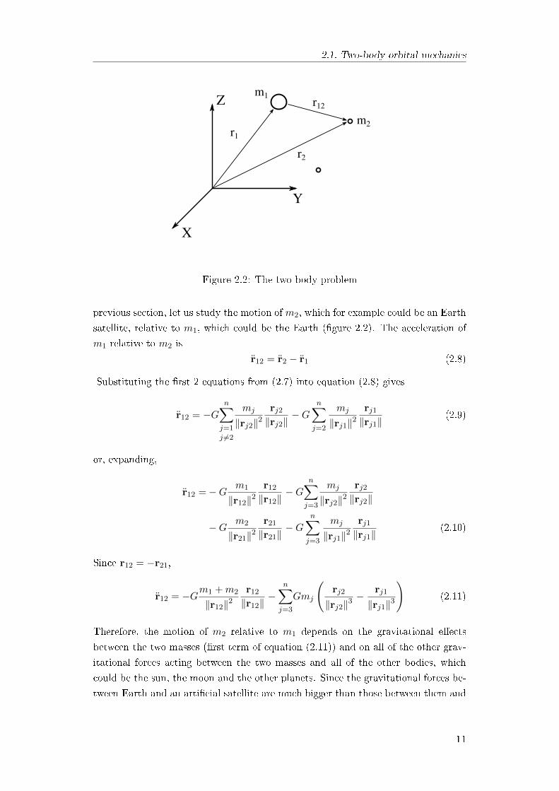
Figure 2.2: The two-body problem
previous section, let us study the motion of m2, which for example could be an Earth
satellite, relative to m1, which could be the Earth (gure 2.2). The acceleration of
m1 relative to m2 is
r12 = r2 − r1 (2.8)
Substituting the rst 2 equations from (2.7) into equation (2.8) gives
r12 = −Gn∑j=1
j 6=2
mj
‖rj2‖2rj2‖rj2‖
−Gn∑j=2
mj
‖rj1‖2rj1‖rj1‖
(2.9)
or, expanding,
r12 =−G m1
‖r12‖2r12
‖r12‖−G
n∑j=3
mj
‖rj2‖2rj2‖rj2‖
−G m2
‖r21‖2r21
‖r21‖−G
n∑j=3
mj
‖rj1‖2rj1‖rj1‖
(2.10)
Since r12 = −r21,
r12 = −Gm1 +m2
‖r12‖2r12
‖r12‖−
n∑j=3
Gmj
(rj2
‖rj2‖3− rj1
‖rj1‖3
)(2.11)
Therefore, the motion of m2 relative to m1 depends on the gravitational eects
between the two masses (rst term of equation (2.11)) and on all of the other grav-
itational forces acting between the two masses and all of the other bodies, which
could be the sun, the moon and the other planets. Since the gravitational forces be-
tween Earth and an articial satellite are much bigger than those between them and
11

2.1. Two-body orbital mechanics
the other bodies, the last term of equation (2.11) represents the perturbing eects.
Replacing r12 with r, that is the vector that goes from the primary body to the
secondary one, m1 with M and m2 with m, and neglecting the perturbing eects,
gives
r = −GM +m
r3r (2.12)
If the mass of the primary body is much bigger than that of the secondary one, we
can make another simplifying assumption by saying that G (M +m) ≈ GM . Let us
also introduce a convenient parameter, µ, called the gravitational parameter:
µ ≡ GM (2.13)
For any given body, its gravitational parameter is the product of the gravitational
constant and its mass. Table 2.1 lists the gravitational parameters of the sun and
the planets of our solar system. We can now write equation (2.12) as
r +µ
r3r = 0 (2.14)
Equation (2.14) is the restricted two-body equation of motion, where the term re-
stricted indicates that the gravitational pull of m on M is neglected.
Table 2.1: Gravitational parameter of the Sun and planets
Planet Mass/Mass Earth Gravitational parameter [km3/s2]
Sun 333432 1.327× 10¹¹
Mercury 0.056 2.232× 10⁴
Venus 0.817 3.257× 10⁵
Earth 1 3.986× 10⁵
Mars 0.108 4.305× 10⁴
Jupiter 318.0 1.268× 10⁸
Saturn 95.2 3.795× 10⁷
Uranus 14.6 5.820× 10⁶
Neptune 17.3 6.896× 10⁶
2.1.3 Potential energy
The mechanical work per unit mass done by the gravitational force of the primary
body to move the secondary one from a certain point 1 to point 2 is
L =
ˆ 2
1Fg · ds =
ˆ 2
1− µr3
r · ds =
ˆ 2
1− µr3dr =
µ
r2− µ
r1(2.15)
and does not depend on the trajectory of the body. Therefore, the gravitational eld
is conservative and an object moving through only a gravitational eld does not lose
12

2.1. Two-body orbital mechanics
or gain any mechanical energy, but only exchanges its kinetic and potential energy.
As a matter of fact, the work done by the gravitational force can be expressed as the
opposite of the change of potential energy of the body. Per unit mass one has
L = −∆Eg = − (Eg2 − Eg1) = Eg1 − Eg2 (2.16)
When the work is positive and the secondary body moves towards the primary one,
the potential energy decreases, whereas when the secondary body moves away the
potential energy increases. Therefore, from equations (2.15) and (2.16) one has
Eg1 − Eg2 = − µr1
+µ
r2(2.17)
with the specic potential energy dened as
Eg = −µr
+ c (2.18)
where specic indicates it is per unit mass and c is an arbitrary constant. Its
values depends on which reference point is used as zero of potential energy. This
choice is completely arbitrary, but in astrodynamics c is conventionally set to zero.
This makes the zero reference of potential energy at innity from the primary body
and also makes the potential energy always negative. Therefore, one has
Eg = −µr
(2.19)
2.1.4 Constants of the motion
Of course, the objective of the problem is to solve the equation of motion in order
to describe the trajectory of the satellite. Before doing that, let us collect some useful
insights into the physics of a body moving in a gravitational eld.
Let us take the scalar product of the equation of motion with the rst derivative
of the position vector, that is the velocity vector:
r · r +µ
r3r · r = 0 (2.20)
Since v = r and, given any vector a, one has a · a = aa,
vv +µ
r3rr = 0 (2.21)
that is,d
dt
(v2
2− µ
r
)= 0 (2.22)
13

2.1. Two-body orbital mechanics
The term within the brackets is the specic mechanical energy of the body
E =v2
2− µ
r(2.23)
that is the sum of the kinetic and potential energy. As already anticipated, during
the motion it is constant and an object moving under the inuence of gravity alone
exchanges one form of energy with the other.
Let us now take the vector product of r with the equation of motion,
r× r + r× µ
r3r = 0 (2.24)
which gives
r× r = 0 (2.25)
that is,d
dt(r× v) = 0 (2.26)
Therefore, the specic angular momentum
h = r× v (2.27)
is a constant vector. Since h is constant and must be always perpendicular to both
r and v, the motion of the secondary body must occur in the same plane, that is r
and v must remain in the same plane. This plane is known as orbital plane. This
result is common to all central forces, since there's no torque acting on the body.
The magnitude of the specic angular momentum vector can be expressed with the
ight path angle. As shown in gure 2.3, it's always possible to dene a vertical
direction and an horizontal direction, no matter where the secondary body is located
in space. In the orbital plane, the local vertical at the location of the S/C is the same
as the direction of r and the local horizontal is perpendicular to it. Thus, one may
always say up by meaning away from the center of the primary body and down
by meaning towards its center. Therefore, the direction of the velocity vector can
be specied by the angle ϕ it makes with the local horizontal, known as ight path
angle. From the denition of cross product the magnitude of h is
h = rv sin (π − ϕ) = rv cosϕ (2.28)
The angle π − ϕ is also referred to as γ, the zenith angle. However, it's more
convenient to express the specic angular momentum in terms of ϕ.
The cross product of the equation of motion with h gives
r× h +µ
r3r× h = 0 (2.29)
14

2.1. Two-body orbital mechanics
r
vφ
loca
l ver
tical
local horizontal
Figure 2.3: Flight path angle
which can be rewritten as
d
dt(r× h) +
µ
r3r× (r× r) = 0 (2.30)
We can now use equations (A.6) and (A.16) from Appendix A to rewrite equation
(2.30) as
d
dt(r× h) +
µ
r3r× (r× r) =
d
dt(r× h) +
µ
r3[(r · r) r− (r · r) r] =
d
dt(r× h) + µ
(r
r2r− r
r
)=
d
dt(r× h)− µ d
dt
(r
r
)=0 (2.31)
By integrating, one nds that the vector
B = v × h− µr
r(2.32)
is another constant of the motion in the two-body problem.
2.1.5 Trajectory equation
Let us now take the scalar product of r with equation (2.32),
r ·B = r · v × h− r · µr
r(2.33)
15

2.1. Two-body orbital mechanics
Circle
Ellipse
Parabola
Hyperbola
Figure 2.4: Conic sections
By using equation (A.18) one has
rB cos ν = h2 − µr (2.34)
where ν is the angle between B and r. Let us nally solve for r and obtain
r =h2/µ
1 + B/µ cos ν(2.35)
Equation (2.35) is the trajectory equation in polar coordinates and it describes how
the secondary body moves with respect to the primary body. Before making any
observation with regard to this equation, let us revise some basic concepts of conic
sections.
2.1.6 Conic sections
A conic section can be dened as a curve obtained from the intersection of a
plane and a right circular cone (gure 2.4). If the plane crosses one half of the cone
the section is called ellipse. If the plane is also parallel to the base of the cone, the
section is a circle. On the other hand, if the plane is parallel to a line in the surface
of the cone, the section is a parabola. Finally, if the plane cuts across both halves of
the cone, the section is called hyperbola and it has two branches. There also can be
degenerate conics, like one or two straight lines and a single point, when the plane
cuts across the apex of the cone. The mathematical translation of this geometric
denition is the following. A conic section is the locus of points such that the ratio
of the distance r from a given point, called focus, to its distance d from a given line,
16

2.1. Two-body orbital mechanics
p
s
r
d
ν
Figure 2.5: Conic sections parameters
called directrix, is a positive constant e, called eccentricity :
e =r
d(2.36)
Letting s be the distance between the focus and the directrix, as shown in gure
2.5, one has
d = s− r cos ν (2.37)
which can be rewritten as
r =p
1 + e cos ν(2.38)
where p = es is a geometrical constant of the conic section known as parameter or
semilatus rectum. Equation (2.38) is the general equation of a conic section in polar
coordinates with the origin located at a focus and the polar angle ν dened as the
angle between the position vector and the point of the conic section nearest to the
focus. Equation (2.38) is formally identical to the trajectory equation. This veries
Kepler's rst law and extends it to include orbital motion along any conic section,
not just ellipses. The semilatus rectum of the conic, that is the distance between
the focus and the point in the trajectory where ν = π/2, is related to the angular
momentum of the S/C:
p =h2
µ(2.39)
In addition, the eccentricity of the conic section is the magnitude of B/µ and
e =B
µ(2.40)
is called eccentricity vector.
17

2.1. Two-body orbital mechanics
2c
2a
2pF' F
2a
2pF'F
2pFa=∞
c=∞
-2a
-2c
2pF F'
2b
Figure 2.6: Geometry of conic sections
Among the conic parameters, for orbital mechanics the directrix has no physical
signicance. On the other hand, the focus, the eccentricity and the semilatus rectum
are important parameters. Figure 2.6 shows the geometrical parameters of conic
sections. Physically, the prime focus F represents the location of the primary body
and the second focus F ′ has no physical signicance. The parabola constitutes the
limit between closed and open orbits and its second focus lies at an innite distance
from the prime. The length of the chord denoted as 2p is the latus rectum and
the length of the chord between the line of the foci and its intersection with the
conic section, denoted as 2a, is the major axis. Following from this denition, the
dimension a is known as semimajor axis. The semimajor axis of the circle is its
radius, for the parabola it is innite and for the hyperbola is taken as negative. The
width of an ellipse at the center, denoted as 2b, is calledminor axis and the dimension
b is known as semiminor axis. The distance between the two foci is denoted as 2c.
For the circle it is zero, as the two foci coincide, for the parabola it is innite and
for the hyperbola it is taken as negative. Following from the denition of a conic
section one can easily prove that
e =c
a(2.41)
and
p = a(1− e2
)(2.42)
18

2.1. Two-body orbital mechanics
always hold true except for the parabola. The extreme points of the major axis are
called apses. The point nearest the prime focus is called periapsis and the point
farthest from the prime focus is called apoapsis. This nomenclature may also vary
depending on the primary body. As a matter of fact, if the primary body is the
Earth we may also specify it by saying perigee and apogee, or, in the case of the Sun,
perihelion and apohelion. For the circle this nomenclature is obviously not denable
and the apoapsis has no meaning for open trajectories.
From equation (2.35) we see that the radius reaches its minimum value for ν = 0.
Therefore, the eccentricity vector is directed towards the periapsis. The polar angle
ν, between the position vector and the vector the points towards the periapsis, is
known as true anomaly. The distance from the primary body to either periapsis or
apoapsis can be obtained by inserting 0 or π as true anomaly in equation (2.35).
Therefore, for any conic section one has
rP =p
1 + e(2.43)
rA =p
1− e(2.44)
where the subscripts P and A indicate the periapsis and the apoapsis, respectively.
Combining equations (2.43) and (2.44) with equation (2.42) gives
rP = a (1− e) (2.45)
rA = a (1 + e) (2.46)
2.1.7 Relating energy to the geometry of an orbit
The total specic energy can be evaluated at any point in the trajectory. In
particular, at the periapsis one has
E =v2P
2− µ
rP(2.47)
The velocity at the periapsis can be expressed in terms of specic angular momentum.
From equation (2.28) one has
vP =h
rP cosϕ(2.48)
From the denition of ight path angle, one has
tanϕ =vrvt
(2.49)
where
vr = v sinϕ (2.50)
19

2.1. Two-body orbital mechanics
is the radial component of the velocity and
vt = v cosϕ (2.51)
its tangential component. Substituting equation (2.40) in (2.35) we can write
r (1 + e cos ν) =h2
µ(2.52)
Dierentiating both side,
r (1 + e cos ν)− rνe sin ν = 0 (2.53)
Since vr = r and vt = rν, one has
vrvt
=e sin ν
1 + e cos ν(2.54)
Substituting (2.54) into (2.49) gives
tanϕ =e sin ν
1 + e cos ν(2.55)
At the periapsis one has
ϕP =e sin 0
1 + e cos 0= 0 (2.56)
We can now use this result and rewrite (2.48) as
vP =h
rP(2.57)
Let us know substitute (2.57) into (2.47) and obtain
E =h2
2r2p
− µ
rP(2.58)
Combining equations (2.39) and (2.42) gives
h2 = µa(1− e2
)(2.59)
Let us now substitute equations (2.59) and (2.45) into (2.58) to nally obtain
E = − µ
2a(2.60)
Equation (2.60) is valid for all the types of orbit. For closed orbits (circle and ellipse)
a is positive and the total mechanical energy of the S/C is negative, while for the
parabola a is innite and the energy is zero and for the hyperbola a is negative and
20

2.1. Two-body orbital mechanics
the energy is positive. Combining equations (2.59) and (2.60) gives
e =
√1 +
2Eh2
µ2(2.61)
For any conic orbit, the energy and the angular momentum determine the eccentricity
of the orbit, which species the shape of the orbit. When the orbit is closed E is
negative and e < 1; if E is positive the orbit is an hyperbola e > 1; if E is zero the
orbit is a parabola and e = 1. However, when h is zero e is also equal to 1; as a
matter of fact, in this case the orbit is a degenerate conic (straight downfall to the
primary body). Therefore, all parabolas have e = 1 but an orbit whose eccentricity
is 1 may not be a parabola.
2.1.8 Closed orbits
The orbits of all Earth satellites are ellipses. Furthermore, the orbits object of
this thesis are almost circular and their eccentricity is close to zero. For this reason,
this section will go over some basic concepts of closed orbits, whereas parabolas and
hyperbolas won't be treated in this work.
2.1.8.1 Period of an elliptical orbit
Since an ellipse is a closed curve, a S/C on an elliptical orbit travels the same
path at each revolution. The time it takes the S/C to complete one revolution is
called the period. From equations (2.28) and (2.51) we know that
h = rvt (2.62)
Using vt = rν we can write
h = r2dν
dt(2.63)
The dierential element of area dA swept out by r as it moves through an innitesimal
angle dν is given by
dA =r2
2dν (2.64)
We can now use this expression to rewrite 2.64 as
dA
dt=h
2(2.65)
which proves Kepler's second law that the radius vector sweeps equal areas in equal
time, as h is a constant. Rewriting equation (2.65) as
dt =2
hdA (2.66)
21
2.1. Two-body orbital mechanics
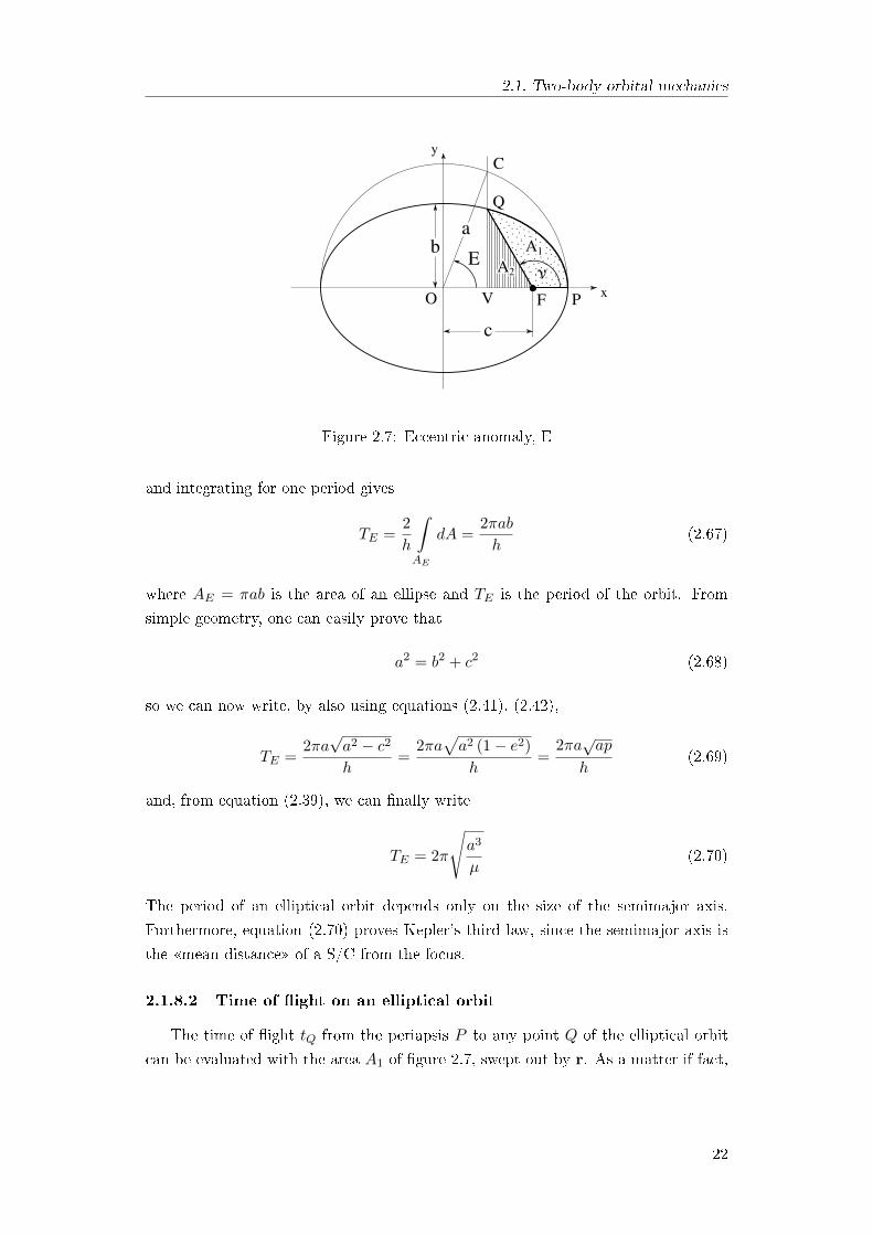
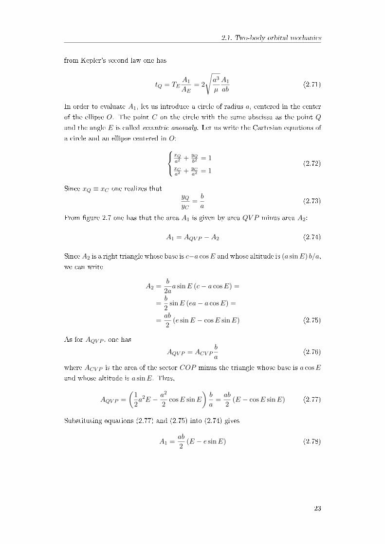
O P
C
Q
Eν
x
y
ab
F
A2
A1
V
c
Figure 2.7: Eccentric anomaly, E
and integrating for one period gives
TE =2
h
ˆ
AE
dA =2πab
h(2.67)
where AE = πab is the area of an ellipse and TE is the period of the orbit. From
simple geometry, one can easily prove that
a2 = b2 + c2 (2.68)
so we can now write, by also using equations (2.41), (2.42),
TE =2πa√a2 − c2
h=
2πa√a2 (1− e2)
h=
2πa√ap
h(2.69)
and, from equation (2.39), we can nally write
TE = 2π
√a3
µ(2.70)
The period of an elliptical orbit depends only on the size of the semimajor axis.
Furthermore, equation (2.70) proves Kepler's third law, since the semimajor axis is
the mean distance of a S/C from the focus.
2.1.8.2 Time of ight on an elliptical orbit
The time of ight tQ from the periapsis P to any point Q of the elliptical orbit
can be evaluated with the area A1 of gure 2.7, swept out by r. As a matter if fact,
22
2.1. Two-body orbital mechanics
from Kepler's second law one has
tQ = TEA1
AE= 2
√a3
µ
A1
ab(2.71)
In order to evaluate A1, let us introduce a circle of radius a, centered in the center
of the ellipse O. The point C on the circle with the same abscissa as the point Q
and the angle E is called eccentric anomaly. Let us write the Cartesian equations of
a circle and an ellipse centered in O:xQa2 +
yQb2
= 1
xCa2 + yC
a2 = 1(2.72)
Since xQ ≡ xC one realizes thatyQyC
=b
a(2.73)
From gure 2.7 one has that the area A1 is given by area QV P minus area A2:
A1 = AQV P −A2 (2.74)
Since A2 is a right triangle whose base is c−a cosE and whose altitude is (a sinE) b/a,
we can write
A2 =b
2aa sinE (c− a cosE) =
=b
2sinE (ea− a cosE) =
=ab
2(e sinE − cosE sinE) (2.75)
As for AQV P , one has
AQV P = ACV Pb
a(2.76)
where ACV P is the area of the sector COP minus the triangle whose base is a cosE
and whose altitude is a sinE. Thus,
AQV P =
(1
2a2E − a2
2cosE sinE
)b
a=ab
2(E − cosE sinE) (2.77)
Substituting equations (2.77) and (2.75) into (2.74) gives
A1 =ab
2(E − e sinE) (2.78)
23

2.1. Two-body orbital mechanics
Finally, substituting into equation (2.71) yields
tQ =
√a3
µ(E − e sinE) =
M
n(2.79)
where, according to Kepler, the mean motion n is
n =
õ
a3(2.80)
and the mean anomaly M is
M = E − e sinE (2.81)
In order to use equation (2.79) to determine the time of ight, we have to relate the
eccentric anomaly to the true anomaly. From gure 2.7,
cosE =c+ r cos ν
a=ea+ r cos ν
a(2.82)
Combining equations (2.38) and (2.42) gives
r =a(1− e2
)1 + e cos ν
(2.83)
Therefore, we can rewrite equation (2.82) as
cosE =e+ cos ν
1 + e cos ν(2.84)
and the correct quadrant for E is obtained by considering that ν and E are always
in the same half-plane.
2.1.8.3 Circular orbit
The circular orbit is a special case of an elliptical orbit and the semimajor axis
of a circle is just its radius, so equation (2.70) becomes
Tc = 2π
√r3
µ(2.85)
The speed of a S/C in a circular orbit vc is called circular speed, which can be easily
derived from equations (2.23) and 20:
E =v2c
2− µ
r= − µ
2a(2.86)
Since a = r we have
vc =
õ
r(2.87)
24

2.2. Coordinate systems
The greater the radius the less is the speed of a S/C in a circular orbit. For a S/C
in LEO the circular speed may vary from 7.7 km/s at 200 km altitude to 6.9 km/s at
2000 km.
The angular velocity of a S/C in a circular orbit is
nc =vcr
=
õ
r3(2.88)
The true anomaly swept out by the radius vector in tQ is
ν = nctQ (2.89)
Equation (2.89) unveils the meaning of the mean anomaly M . As a matter of fact,
from equations (2.80) and (2.88), the mean motion n is, for a given orbit, the angular
velocity of a circular orbit with radius equal to the semimajor axis. Therefore,
rewriting equation (2.79),
M = ntQ (2.90)
and comparing it to equation (2.89) one realizes that the mean anomaly of a given
orbit is, after tQ time is passed from the passage at the periapsis, the same as the
true anomaly swept out by a S/C in a circular orbit with the same semimajor axis
during tQ.
2.2 Coordinate systems
Depending on the type of space mission, it is necessary to provide a suitable
coordinate system and a set of coordinates. The choice of a suitable coordinate
system is far from being a simple task, as the spatial description of an orbit ideally
requires an inertial reference frame. However, any coordinate system one can dene
has a certain degree of uncertainty to its inertial qualities. In practice, a coordinate
system centered in the primary body and with axes pointing a xed direction with
respect to the xed stars does the job of being almost inertial. Rectangular coor-
dinate systems are the most used in astrodynamics, although sometimes spherical
polar coordinates are more practical. In order to describe a rectangular coordinate
system, one has to give the position of the origin, the orientation of the fundamental
plane, on which the X and the Y axes lie, the positive direction of the Z axis and the
principal X direction (assuming X, Y and Z form a right handed set of coordinate
axes).
2.2.1 The heliocentric-ecliptic coordinate system
The origin of the heliocentric-ecliptic coordinate system is the center of the Sun.
The fundamental plane is the ecliptic, that is the plane the Earth orbits on. As
25

2.2. Coordinate systems
first dayof spring
first dayof winter
first dayof autumn
first dayof summer
g1
g2
g3
direction ofvernal equinox
SUN
Figure 2.8: Heliocentric-ecliptic coordinate system (seasons are for Northern Hemi-sphere)
shown in gure 2.8, the direction of the the X axis, labeled as g1, is given by the
line of intersection between the ecliptic plane and the Earth's equatorial plane. The
positive direction of g1, called the vernal equinox direction (symbol because it
used to point in the direction of the constellation of Aries), is given by a line that, on
the rst day of spring points, from the center of the Earth points towards the center
of the Sun. As the Earth's axis precesses over the centuries, the line of intersection
between the ecliptic and Earth's equatorial plane slowly drifts clockwise in what
is known as precession of the equinoxes. Therefore, this coordinate system is not
really inertial and, where precision is required, the set of coordinates of an object
are usually specied by saying they were based on the vernal equinox direction of a
given year, or epoch.
2.2.2 The geocentric-equatorial coordinate system
The origin of the geocentric-equatorial coordinate system (gure 2.9) is the center
of the Earth. The fundamental plane is the equator and the positive X axis points
in the vernal equinox direction. The Z axis points in the direction of the north
pole. Therefore, this coordinate system is not turning with the Earth, but rather it
is xed with respect to the stars (neglecting the precession of the equinoxes). This
reference system, dened by unit vectors I, J and K, is obviously extremely useful
for describing the motion of Earth's satellites.
2.2.3 The right ascension-declination coordinate system
The right ascension-declination coordinate system (gure 2.10) is strictly related
to the geocentric-equatorial system. The fundamental plane is the celestial equator,
26

2.2. Coordinate systems
JI
K
x
y
z
Figure 2.9: Geocentric-equatorial coordinate system
I
J
K
α
δ
Figure 2.10: Right ascension-declination coordinate system
i.e. the extension of the equatorial plane to a ctitious sphere of innite radius
known as celestial sphere. The projection of an object on the celestial sphere is
described by two angles, called right ascension and declination. The right ascension
α is measured eastward in the plane of celestial equator from the vernal equinox
direction. The declination δ is measured northward from the celestial equator to the
line from the origin of the system to the projection of the object on the celestial
sphere. Since the celestial sphere is innite, its center may be any point. Therefore,
we may choose the center of the Earth as origin of the system as well as a point on
its surface.
27

2.2. Coordinate systems
xWGS84
yWGS84
zWGS84
La
Lo
r
Figure 2.11: WGS 84
2.2.4 The world geodetic system 84
The origin of World Geodetic System 84 (WGS 84) is the center of mass of the
Earth. The fundamental plane is the equatorial plane and the positive X axis points
towards the intersection between the equatorial plane and the Greenwich meridian.
Therefore, this coordinate system rotates about its Z axis with the same angular
velocity as the Earth. Any point can be identied with a radius r and two angles,
Lo (Longitude) and La (Latitude), as shown in gure 2.11.
2.2.5 The perifocal coordinate system
The origin of the perifocal coordinate system (gure 2.12) is the center of the
primary body. The fundamental plane is the plane of the orbit of the secondary body.
The X axis (unit vector p) points towards the periapsis; the Y axis (unit vector q)
lies in the orbital plane and its rotated in the direction of the orbital motion. The
positive direction of the Z axis (unit vector w) is the positive direction of the angular
momentum vector. The vector r is given by
r = r cos νp + r sin νq + 0w (2.91)
Taking the time derivative, one nds that v is given by
v = (r cos ν − rν sin ν) p + (r sin ν + rν cos ν) q + 0w (2.92)
Since vr = r and vt = rν one has
v = (vr cos ν − vt sin ν) p + (vr sin ν + vt cos ν) q + 0w (2.93)
28

2.2. Coordinate systems
p
r
q
ν
Figure 2.12: Perifocal coordinate system
Combining equations (2.28), (2.35) and (2.51)gives
vt =h
r=µ
h(1 + e cos ν) (2.94)
From equation (2.54) one has
vr = vte sin ν
1 + e cos ν(2.95)
Combining (2.94) and (2.95) yields
vr =µ
he sin ν (2.96)
Since ϕ = arctan (vr/vt), from equation 2.96 we deduce that ϕ is negative when sin ν
is negative and vice versa: ϕ > 0 if 0 < ν < π
ϕ < 0 if π < ν < 2π(2.97)
We can nally insert (2.94) and (2.96) into equation (2.93) to obtain
v = −µh
sin νp +µ
h(e+ cos ν) q + 0w (2.98)
If we know calculate
r · v =µ
hre sin ν (2.99)
29

2.3. Classical orbital elements
J
I
K
n
e
p
Ω
ω
r νih
w
equato
rial p
lane
S/C
Figure 2.13: Classical orbital elements
we realize that, from equation (2.97),ϕ > 0 if r · v > 0
ϕ < 0 if r · v < 0(2.100)
2.3 Classical orbital elements
The shape and the orientation of an orbit, as well as the position of a S/C on
that orbit, are completely described by the position vector and the velocity vector.
Indeed, any consistent set of six parameters can describe a two-body problem orbit.
Five independent quantities unambiguously dene an orbit's shape and orientation,
and a sixth quantity is needed to pinpoint the position of a S/C along that orbit.
Using the position vector and the velocity vector (together they give six independent
quantities) is extremely unpractical and other six parameters are preferred: the
classical orbital elements (gure 2.13). These parameters are obviously dependent
on r and v and can be determined directly from them. The classical orbital elements
are:
1. a, semimajor axis. It denes the dimension of the orbit.
2. e, eccentricity. It denes the shape of the orbit.
3. ı, inclination. It is dened by the angle between the K unit vector and the and
30

2.3. Classical orbital elements
the angular momentum vector:
ı = arccos
(K · h
h
)(2.101)
The inclination is always greater than or equal to zero radians and less than
or equal to π radians: 0 ≤ ı ≤ π
4. Ω, right ascension of the ascending node (RAAN). It is dened as the angle
in the fundamental plane between the I unit vector and the point where the
S/C crosses through the fundamental plane in a northerly direction, hence
ascending, measured counterclockwise when viewed from the north side of
the fundamental plane. Mathematically, we can dene the line of nodes with
unit vector
n =K× h
‖K× h‖(2.102)
pointing towards the ascending node. Following this denition, we can writeΩ = arccos (I · n) if n · J ≥ 0
Ω = 2π − arccos (I · n) if n · J < 0(2.103)
since Ω can assume any value from zero radians to 2π radians.
5. ω, argument of periapsis. It is dened as the angle in the plane of the orbit
of the S/C between the ascending node and the periapsis, measured in the
direction of the motion of the S/C. Mathematically,ω = arccos (n · p) if p ·K ≥ 0
ω = 2π − arccos (n · p) if p ·K < 0(2.104)
6. ν, true anomaly. Given the other orbital elements, it pinpoints the position of
the S/C along the orbit. The mathematical denition is, taking into account
equation (2.100), ν = arccos(rr · p
)if r · v ≥ 0
ν = 2π − arccos(rr · p
)if r · v < 0
(2.105)
The orbital elements a and e dene the geometry of the orbit, that is the dimension
and the shape. The orbital elements i, Ω and ω dene the orientation of the orbit
and, nally, ν reveals where the S/C is along the orbit.
Sometimes, other angle are also used. The angle
Π = Ω + ω (2.106)
31

2.4. Perturbations
is known as longitude of periapsis. It is the angle from I to periapsis, measured in
the equatorial plane and then in the orbital plane. If the orbit is equatorial, that is
the inclination is zero, the line of nodes is not denable and it is convenient to use
this angle.
If the orbit is circular, the argument of periapsis ω is not denable and it is
convenient to use the angle
ϑ = ω + ν (2.107)
known as argument of latitude at epoch, that is the angle in the plane of the orbit
between the ascending node and the radius vector at a particular time (epoch).
In the case of circular orbit Π is not denable, whereas for equatorial orbit µ is
not denable. Therefore, in the case of circular equatorial orbit, it is convenient to
use the angle
l = Ω + ω + ν (2.108)
also known as true longitude at epoch.
2.4 Perturbations
So far we have discussed trajectories that describe the relative motion of two
spherically symmetric bodies under the action of gravity alone. However, real S/C
trajectories are not described accurately by the two-body restricted problem. As a
matter of fact, a S/C is subject to several perturbations, such as the presence of
other attractive bodies, atmospheric drag and lift, the asphericity of the attractive
bodies, solar radiation eects, magnetic eects and thrust. These perturbations,
dened as deviation from the expected motion, may have dierent consequences on
the trajectory of a S/C depending on the space mission. However, in the short run the
orbits of planets and satellites are well approximated by the two-body problem, which
makes it very convenient to describe the motion of celestial bodies. Nevertheless, in
the long run, the perturbations will make the trajectory of the S/C very dierent
from the one predicted by the two-body problem. The orbital elements slowly change
and the S/C appears to continuously pass from a Keplerian orbit to another. Given
a specic time, the Keplerian orbit that has the same orbital elements of the real
perturbed trajectory is called osculating orbit. Following this denition, the orbital
elements of the S/C at a given time are the osculating orbital elements. Generally
speaking, the variation of an orbital element can be secular, i.e. it follows a linear
trend with time, or it can be subject to long period oscillations as a result of the
interaction with the variation of other orbital elements, or also subject to short-
period oscillations, usually caused by phenomena that periodically occur during each
revolution. In all cases, the restricted two-body equation of motion can be formally
32

2.4. Perturbations
written as
r = − µr3
r + fP (2.109)
where fP is the perturbing acceleration. In general, the equation doesn't have an
analytical solution and dierent techniques can be adopted to integrate it. These
techniques are referred to as special perturbations and general perturbations. Special
perturbations methods consist in the numerical integration of the equation of motion
and yield the trajectory of a S/C given a set of initial condition at a particular
time, therefore obtaining a specic solution for a well-dened case. On the other
side, general perturbation methods provide an approximated analytical solution by
expanding perturbing accelerations into series, which are suitably truncated and
integrated.
2.4.1 Variation of parameters
As already discussed, a two-body problem orbit can be described by any suitable
set of six parameters. The variation of parameters method describes how any of
these sets of parameters vary with time as a result of perturbations. The method
consists in the analytical description of the rate of change of the parameters due to
the perturbations. Since in this work the method will be applied with the classical
orbital elements, it can also be called variation of elements. In addition, this method
can be considered either as a special perturbation method or a general perturbation
method, depending on how the expression that the method yields are then integrated.
This methodology is associated with two formulations; the rst one leads to theGauss
planetary equations, which relate the components of the perturbing acceleration to
the rate of change of the orbital elements; the second one, not of interest for this
work, leads to the Lagrange planetary equations.
2.4.1.1 The Gauss planetary equations
As already stated, the Gauss planetary equations relate the components of a
perturbing acceleration to the rate of change of the orbital elements. Depending on
convenience, the perturbing acceleration can be projected in two dierent ways. One
coordinate system has its principle axis R with unit vector R along the instantaneous
radius vector r. The axis T with unit vector T is rotated 90° in the orbital plane
in the direction of motion. The third axis W with unit vector W is perpendicular
to the other two. The other coordinate system has its principle axis V with unit
vector V along the instantaneous velocity vector v. The axis N, with unit vector N,
is rotated through a 90° angle in the orbital plane about W. The third axis W is
the same as for the other coordinate system. Therefore, following this denitions we
have fP = fRR + fTT + fWW = fV V + fNN + fwW. The relations between the
two types of projections are
33

2.4. Perturbations
fR =h
pV[(e sin ν) fV − (1 + e cos ν) fN ] (2.110)
fT =h
pV[(1 + e cos ν) fV + (e sin ν) fN ] (2.111)
The derivation of the rate of change of the orbital elements, shown in depth in [25],
leads to the following results:
a =2a2
õp
[(e sin ν) fR −
(pr
)fT
]=
(2a2V
µ
)fV
e =
√p
µ
[(sin ν) fR +
(r
p
)(e cos2 ν + 2 cos ν + e
)fT
]=
=1
V
[2 (e+ cos ν) fV −
(a sin ν
r
)fN
]ı =
rõp
cos (ω + ν) fW
Ω =r√µp
sin (ω + ν)
sin (ı)fW (2.112)
ω = −Ω cos ı−
√pµ
e
[(cos ν) fR − sin ν
(1 +
r
p
)fT
]=
= −Ω cos ı+1
eV
[(2 sin ν) fV +
r
p
(2e+ cos ν + e2 cos ν
)fN
]M = n− 2r√
uafR −
√1− e2
(ω + Ω cos ı
)=
= n− 2√
1− e2
V
[(er sin ν
p
)fV − fN
]−√
1− e2(ω + Ω cos ı
)Where the mean anomaly is used instead of the true anomaly (they are related by
equations (2.81) and (2.84)).
By looking at the equation for the rate of change of the semimajor axis, one
notes that the only component of the perturbing acceleration that has a role in
its variation is the one along the velocity vector. The eccentricity can be varied
by either a V component or a N component. However, they have dierent eects
depending on where the S/C is along the orbit. One interesting observation is that the
geometry of the orbit, i.e. its dimension and its shape, is only changed by perturbing
accelerations in the orbital plane. The equations for the rate of the inclination
and RAAN show that the orbital plane is changed by a perturbing acceleration
along W; depending on where the S/C is along the orbit, dierent eects on the
orbital plane change can be obtained. At the ascending node, that is when ν = −ω,a perturbing acceleration along W varies only the inclination. At the antinodes,
namely at ∆ν = π/2 from the nodes, a perturbing acceleration along W varies only
34

2.4. Perturbations
the RAAN. Given a certain fW , the cost of changing Ω is lower if the inclination of
the orbit is lower. The argument of periapsis is varied by a change of RAAN and
also by in-plane perturbing accelerations. The rate of change of the mean anomaly
depends on in-plane perturbing accelerations and on ω and Ω variations.
2.4.2 Perturbations in LEO
In LEO the most important perturbing forces acting on a S/C are due to aerody-
namic eects, asphericity of the Earth, solar radiation and electromagnetic eects.
In this thesis, only the rst two will be accounted for, as the latter are usually quite
small and negligible. Indeed, electromagnetic eects have a far bigger impact on the
attitude dynamics of a S/C than they do on its trajectory.
2.4.2.1 Atmospheric drag
Since in most cases aerodynamic lift is negligible for satellites, only the eects
of drag will be analyzed in this work. The analytic formulation of the perturbing
acceleration due to atmospheric drag is not a simple task, as many parameters that
dene it are aicted by uncertainties. As a matter of fact, the aerodynamic forces
acting on a S/C are dependent on atmospheric uctuation, the frontal area of the
S/C and the drag coecient. The residual atmosphere in LEO is characterized by a
density so low that conventional uid mechanics is not applicable, as the interaction
between the S/C and the atmosphere has to be evaluated at the molecular level.
Without losing generality, the perturbing acceleration due to drag is given by
v = −1
2ρSCDm|v − vatm|2
v − vatm
|v − vatm|(2.113)
where CD is the drag coecient associated with A, m is the mass of the S/C, vatm
is the absolute velocity of the atmosphere and ρ is the atmospheric density at the
altitude of the S/C. The drag coecient depends on the type of reection of the
particles that impact the surface of the S/C and typically it's close to the value 2.2.
The atmospheric density depends on a vast variety of factors, such as altitude, season,
local solar time, solar activity. It's evident that its exact value is never accurately
predicted and, as a consequence, the eect of drag can solely be roughly estimated.
S is the projection of the area of the satellite perpendicular to the vector v − vatm,
that is the relative velocity of the S/C with respect to the atmosphere. The frontal
area S depends on the attitude of the satellite. In this work, it will also depend on
the deployment of a sail. By introducing the vector vrel = v − vatm we can rewrite
equation (2.113) as
v = −1
2ρSCDm|vrel|vrel (2.114)
35

2.4. Perturbations
2.4.2.2 Asphericity of the Earth
The Earth doesn't have neither geometrical symmetry nor mass symmetry. As a
matter of fact, it is an oblate body, attened at the poles and bulged at the equator.
In addition, it is characterized by asymmetrical density variations. Therefore, the
expression for the gravitational potential is not quite the one introduced in the two-
body problem. The equatorial bulge produces a torque on the satellite and the orbit
plane precesses. In addition, the line of the nodes moves westward for direct orbits,
that is whose inclination is less than 90°, and westward for retrograde orbits, that is
whose inclination is more than 90°. The gravitational potential of the Earth in the
WGS84 coordinate system can be expressed by
Eg =µ
r− µ
r
∞∑n=2
Jn
(r⊕r
)nPn sinLa
− µ
r
∞∑n=2
∞∑m=2
Jn,m
(r⊕r
)mPmn sinLa cos [m (Lo− Lom,n)] (2.115)
The function Pn (x) is the Legendre's polynomial of degree n:
Pn (x) =1
2nn!
dn
dxn[(x2 − 1
)](2.116)
whereas Pmn (x) is the associated Legendre's polynomial of degree n and order m:
Pn (x) = (−1)m(1− x2
)m2dm
dxm[Pn (x)] (2.117)
The terms Jn are called zonal harmonics, whereas Jn,m are called tesseral and sec-
torial harmonics for n 6= m and n = m, respectively. The zonal harmonics describe
the asymmetry with respect to the equator and depend on latitude. The tesseral
and sectorial harmonics describe the asymmetry of the Earth about its axis of rota-
tion. The tesseral harmonics depend on latitude and longitude, while the sectorial
harmonics depend on longitude only.
The zonal harmonic J2, which describes Earth's oblateness, is the most important
term and its value (J2 = 1.082629·10−3) is three orders of magnitude greater then any
other. In addition, LEO orbits aren't aected by tesseral and sectorial harmonics, as
their eect is averaged by the rotation of the Earth inside the orbit of the S/C (this
isn't the case for satellites in geostationary orbit, which maintain a xed position
relative to the Earth). In practice, for LEO orbit it is sucient to consider the Earth
as axisymmetric and neglect both tesseral and sectorial harmonics. In addition, if
only J2 is considered, the method of general perturbation yields the following orbital
36

2.4. Perturbations
elements variations after one revolution:
∆Ω = −3πJ2
(r⊕p
)2
cos ı (2.118)
∆ω =3
2πJ2
(r⊕p
)2 (5 cos2 ı− 1
)(2.119)
The regression of the line of the nodes is an important eect on LEO orbits, and its
entity increases as the orbit is less inclined. For direct orbits the line of the nodes
regresses, whereas for retrograde orbits it precesses. On the other hand, the line of
apses precesses for ı < 63.4 or ı > 116.6 and regresses for 63.4 < ı < 116.6. For
either ı = 63.4 or ı = 116.6, that is when 5 cos2 ı − 1 = 0, J2 has no eect on the
line of apses.
37

Chapter 3
Propulsion
Since ADR and OOS missions will require the S/C to perform many LEO trans-
fers, electric propulsion (EP) will be arguably the preferred option. As a matter
of fact, although the acceleration levels EP can achieve are far lower than those of
chemical propulsion, the propellant consumption of electric thrusters is very lim-
ited. Although transfer times will be generally longer than the ones achievable with
chemical propulsion, the low propellant consumption will allow the S/C to complete
more transfers. This chapter will give the reader an insight into the generalities
of space propulsion and will highlight the dierences between chemical and electric
propulsion.
3.1 Generalities of space propulsion
In space there is almost nothing to exchange momentum with. Therefore, the
S/C is an isolated system and the only way to generate thrust consists in having on
board something to exchange momentum with, namely the propellant. The source
of the energy used to accelerate the propellant denes the main two elds of space
propulsion: chemical propulsion and electric propulsion. The energy used to acceler-
ate the propellant comes from a chemical reaction for chemical propulsion, whereas
for electric propulsion it comes from a electric power generator.
Let us consider an isolated S/C, far away from any other mass that could generate
a gravitational pull. The S/C has a certain velocity v at the time t. Let us study a
uni-dimensional case. After an innitesimal time dt the S/C has ejected a mass of
propellant dmp and changes its velocity to v + dv. The mass dmp has a velocity c
with respect to the S/C, thus having a v − c absolute velocity. Let us apply the law
of conservation of momentum:
mv = (m− dmp) (v + dv)− dmp (c− v) (3.1)
38

3.1. Generalities of space propulsion
which rewrites as
mdv = dmpc (3.2)
Let us introduce the propellant mass ow rate:
mp =dmp
dt(3.3)
The dierential dmp can be rewritten as the product of the mass ow rate and dt,
giving
mdv
dt= mpc (3.4)
This equation gives an expression for the product of the mass of the S/C and its
acceleration, that is thrust:
T = mpc (3.5)
In order to accelerate the propellant from zero velocity to c with respect to the S/C,
a certain amount of energy has to be spent. Let us introduce the thrust power:
PT =1
2mpc
2 =1
2Tc (3.6)
which is the power needed to continuously accelerate the propellant from 0 to c.
In reality, the propellant that is being ejected interacts with the propellant inside
the /C. If the exit velocity of the propellant is ue, taking into account the momentum
exchange with the ejected propellant, the thrust formula rewrites as
T = mpue +Ae (pe − p0) (3.7)
where Ae is the exit area and p0 is the atmospheric (null if the S/C is in a void). In
any case, it is far more convenient to use equation (3.5), compressing in c the eects
of accelerating the propellant and the pressure of the ejected propellant. By using
(3.5), the detail on the value of the exit velocity and the value of the exit pressure is
lost. However, this is not a problem as the detail on how thrust is generated is not
of particular interest. As a matter of fact, two thrusters can exert the same thrust
on a S/C with dierent ue and pe, but the eects on the S/C are the same. For this
reason, it is far more useful to dene the ratio between thrust and mass ow rate:
c =T
mp(3.8)
where c is called eective exhaust velocity . If pe = p0, c is exactly equal to the exhaust
velocity. In space propulsion, this is almost always the case (approximately).
39

3.2. Performance of the propulsion system
3.2 Performance of the propulsion system
The aim of the propulsion system is to change the velocity of the S/C. Thus, the
thrust is not itself as much of interest as its eects on the S/C. The integral of thrust
over the complete duration of a mission,
It =
ˆ tf
t0
Tdt (3.9)
is called total impulse. The total mass of propellant used is
mp =
ˆ tf
t0
mpdt (3.10)
The ratio between the total impulse and the weight of the mass of the propellant
used on the surface of the Earth,
Isp =It
mpg0(3.11)
is called specic impulse. Historically, the specic impulse is dened with the weight
instead of the mass of the propellant. If both thrust and mass ow rate are constant
throughout the mission, one has
Isp =It
mpg0=
T∆t
mp∆tg0=
T
mpg0=
c
g0(3.12)
The meanings of Isp and c are fundamentally the same. The specic impulse is
a measure of how eectively the propellant mass is ejected. Let us consider given
mass of propellant mp and let's imagine we want to generate thrust with a certain
eective exhaust velocity c. Let us also imagine that the generated thrust is equal to
the weight of the propellant: T = mpg0. Let us nd how much time the thruster can
give us this level of thrust. From the denition of total impulse, we have ∆t = It/T .
This expression rewrites, using the denition of specic impulse, as ∆t = Ispmpg0/T .
Since T = mpg0, we nally have ∆t = Isp. Given mp, if c increases the same thrust
can be exerted for more time. The specic impulse can be considered as the time
a certain quantity of propellant can give a thrust equal to its weight on Earth. In
practice, if Isp increase, the same thrust can be exerted for more time or more thrust
can be exerted for a given time.
Even though the total impulse It = mpc is a measure of the performance of the
propulsion system, as it shows how it aects the S/C based on how much propellant
is on board and on the value of eective exhaust velocity the system is capable to
achieve, it is not enough to have a complete picture of the performance. As a matter
of fact, the velocity change of the S/C is the primary aim of propulsion. The same
total impulse has dierent eects on dierent S/Cs, depending on the mass. The
40

3.2. Performance of the propulsion system
integral of the acceleration due to thrust over the course of a mission,
∆V =
ˆ tf
t0
T
mdt (3.13)
is called delta-V. It represents the change in velocity that a S/C would be subjected
to if the only force acting on it was thrust parallel to the velocity. The actual change
in velocity depends on all of the other forces that interact with the S/C. However,
the meaning on ∆V is measuring of the eects of thrust. For example, a body in a
gravitational eld will have ∆V = 0 in the absence of thrust, even when accelerating
or decelerating. The delta-V can be rewritten by using equation (3.8):
∆V =
ˆ tf
t0
cmp
mdt (3.14)
The propellant mass ow rate is equal and opposite to the time derivative of the
mass of the S/C:
mp = −dmdt
(3.15)
Substituting equation (3.15) into (3.14) yields
∆V =
ˆ mf
m0
−cdmm
(3.16)
This expression can be simplied by assuming c is a constant. The resulting equation
is the Tsiolkovsky rocket equation:
∆V = c ln
(m0
mf
)(3.17)
which can be written as
mf = m0e−∆V
c (3.18)
The rocket equation relates the initial and the nal mass of a S/C depending on the
delta-V and c. Thus, it gives an expression for the propellant needed for a maneuver:
mp = m0 −mf = m0
(1− e−
∆Vc
)(3.19)
The following table shows the ration between initial and nal mass as a function of
the ratio between ∆V and c:
41

3.2. Performance of the propulsion system
∆V/c mf/m0m0/mf
5 0.0067 1482 0.135 7.391 0.368 2.720.5 0.606 1.650.2 0.819 1.220.1 0.905 1.11
Table 3.1: Results of the rocket equation
Since m0/mf is a measure of the cost of the mission (the more it increases
the more propellant is needed), given a certain ∆V , c shall be comparable. The
bigger the eective exhaust velocity, the lesser propellant is needed for a given mis-
sion/maneuver. The typical delta-V for some missions are shown on the following
table:
Mission ∆V [km/s]
LEO insertion 10Station keeping (1 year) 0.5LEO-GEO (impulsive) 3.5LEO-GEO (low-thrust) 6Earth escape (impulsive) 3.2Earth escape (low-thrust) 8Earth-Mars (impulsive) 5.5Earth-Mars (low-thrust) 6Earth-Jupiter (low-thrust) 16.7Earth-Alpha Centauri 30000
Table 3.2: Typical delta-Vs
As a rst approximation, given the mass of a S/C, the total impulse solely depends
on the delta-V:
It ≈ mavg∆V (3.20)
From the denition of Isp,
mp =It
g0Isp(3.21)
one notes that, given the mission, the mass of propellant is inversely proportional
to the specic impulse of the thruster. Given a certain mission, doubling Isp means
completing the mission with half of the propellant. For chemical propulsion, Isp is
limited by the maximum energy that the chemical reaction can generate (Isp = 450 s
with liquid oxygen LOX and liquid hydrogen LH2). This fact has repercussions on
the ratio m0/mf . For example, insertion in LEO requires ∆V = 10 km/s. By using
LOX/LH2, which by the way is the best combination in terms of Isp, the ratio ∆V/c
42

3.3. Chemical propulsion and electric propulsion
is roughly equal to 2. From table (3.2) we see that the nal mass is limited to a
10% of the initial mass. For bigger delta-Vs chemical propulsion is almost always
not practical. On the other hand, electric propulsion is not characterized by a direct
dependence between the propellant and the energy available. Therefore, bigger c can
be easily obtained.
3.3 Chemical propulsion and electric propulsion
In chemical propulsion a propellant mass ow rate mp reacts and releases chemical
energy, which is converted to kinetic energy by letting the gas expand and accelerate.
The energy balance can be written as
mp
(he +
u2e
2− h0
)= ηmpEch (3.22)
Where Ech is the energy per unit mass released by the reaction, he and h0 are
the specic enthalpy of the propellant when it enters and when it exits the thrust
chamber. The eciency η takes into account how much chemical energy is actually
transformed into enthalpy. By neglecting the enthalpy of the propellant when it
enters the thrust chamber, assuming maximum eciency and substituting c ≈ ue,
we can write
cchemical ≈√
2Ech (3.23)
Equation (3.23) shows that c is limited by the energy of the reaction and gives an
upper limit for c. This is also intuitive, as the energy used to accelerate the propellant
is contained in the propellant itself. Therefore, the extent to which it can accelerate
depends on the energy the propellant itself is capable of releasing. On the other
hand, this fact is what makes chemical rockets extremely scalable, as it's possible to
either increase or decrease the propellant mass ow rate for a given value of c. In
theory, the thrust achievable can be arbitrarily big, with the drawback of having a
large propellant consumption.
As for electric propulsion, the propellant mass ow rate mp receives a certain
amount of electric power PE . The energy balance is:
mpc2
2≈ ηPE (3.24)
While chemical rockets can achieve high values for η, this is not the case for electric
thrusters. As a matter of fact, the transformation from electrical to kinetic energy
is characterized by high losses. From equation (3.24) we have
celectric ≈
√2ηPEmp
(3.25)
43

3.4. Limits of electric propulsion
Theoretically, arbitrary high values of c can be obtained by either increasing PE or
decreasing mp.
In a chemical rocket, the energy available mpEch and requested mpc2/2 are bound
by the mass of propellant. If one increases, the other one increases as well. On the
other side, an electric thruster doesn't have this limitation, as the available power PE
is completely unrelated to the mass of propellant. Therefore, given a certain power,
an electric thruster can accelerate more a smaller mass of propellant, and vice versa.
Substituting T = mpc into equation (3.24) yields
c ≈ 2ηPET
(3.26)
which shows that c can be increased by either increasing PE or decreasing T . This
is the fundamental dierence between chemical and electric propulsion. Chemical
rockets can generate arbitrarily high values of thrust (they span from mN to MN
range) with a limited c, whereas electric thruster can achieve high values of c with the
drawbacks of having on board a power source (solar arrays, typically) and limited
thrust (order of N maximum). The available thrust is bounded by technological
limits, as the increase of PE is accompanied by an increase of the mass of the power
source. The choice between chemical or electric depends on the mission. Certainly,
orbit insertion requires high levels of thrust and chemical is the only option. On
the other hand, an interplanetary transfer can be achieved with a lower propellant
consumption by choosing electric propulsion, taking into account that the mission
will require more time.
3.4 Limits of electric propulsion
Electric propulsion requires a power generator. The total mass m of a S/C can
be broken down in various terms:
m = mu +mp +ms (3.27)
where mu is the mass of the payload, mp is the mass of propellant and ms is the
mass of the power generator. The acceleration due to thrust is
a =T
m(3.28)
which is less than the acceleration the S/C would experience if ms was the only mass
a <T
ms(3.29)
44

3.4. Limits of electric propulsion
With good approximation, the mass of the power generator can be assumed as pro-
portional to the electric power the generator produces:
ms = αPE (3.30)
Lower value of α correspond to a better technology. Therefore, we can write:
a <T
αPE(3.31)
Substituting (3.26) into (3.31) yields
a <T
αTc2η
(3.32)
which rewrites as
a <η
α
2
c(3.33)
The acceleration is limited by the right hand side of the inequality. In order grasp
the orders of magnitude one can expect, let us assume very optimistic values for η
and α. If η = 0.5, α = 1 kg/kW and c = 10 km/s one has
a < 0.1m
s2≈ g0
100(3.34)
where g0 is the gravitational acceleration on the surface of the Earth. This thesis
will deal with orbital maneuvers in LEO. This means that the acceleration due to
thrust will be orders of magnitude less than the one due to gravity. Therefore, we
can expect very gradual changes in the trajectory of the S/C.
45

Chapter 4
Mathematical model
4.1 Atmospheric model
As stated in Section 2.4.2, the atmospheric uctuations that characterize LEOs
are dependent on a vast variety of factors, such as altitude, season, local solar time
and solar activity. Since the evaluation of drag depends on the knowledge of the
atmospheric density, it is necessary to have an atmospheric model that accurately
predicts the density along the orbit of the S/C. Since this thesis is meant to give a
methodology in order to take into account the eects of drag on the optimization
problem, its aim is not to give results for a specic case study. For this reason,
the U.S. Standard Atmosphere 1976 was chosen a suitable atmospheric model. The
methodology is not dependent on the atmospheric model, so any model can be readily
adopted instead of the one chosen here.
The U.S. Standard Atmosphere is an idealized, steady-state representation of
the earth's atmosphere from the surface to 1000 km, as it is assumed to exist in a pe-
riod of moderate solar activity. This atmospheric model was adopted by the United
States Committee on Extension to the Standard Atmosphere (COESA), a group of
organizations which aimed to provide the missile industry a realistic atmospheric
model beyond the altitudes of aircraft operations.
The full detail on how the model is built is in [20]. Using the tabulated data,
the density prole ρ (z) between altitudes from z = 86 km and z = 1000 km can be
calculated with the basic equation form
ρ (z) = eAz4+Bz3+Cz2+Dz+E (4.1)
where the value of the A through E coecients are listed in table 4.1.
46

4.2. Analytical description of the perturbations
Table 4.1: Density formula coecients
Density [kg/m3]
Altitude[km]
A B C D E
86-91 0.000000 −3.322622× 10⁻⁶ 9.111460× 10⁻⁴ −0.2609971 5.94469491-100 0.000000 2.873405× 10⁻⁵ −0.008492037 0.6541179 −23.62010100-110 −1.240774× 10⁻⁵ 0.005162063 −0.8048342 55.55996 −1443.338110-120 0.000000 −8.854164× 10⁻⁵ 0.03373254 −4.390837 176.5294120-150 3.661771× 10⁻⁷ −2.154344× 10⁻⁴ 0.04809214 −4.884744 172.3597150-200 1.906032× 10⁻⁸ −1.527799× 10⁻⁵ 0.004724294 −0.6992340 20.50921200-300 1.199282× 10⁻⁹ −1.451051× 10⁻⁶ 6.910474× 10⁻⁴ −0.1736220 −5.321644500-750 8.105631× 10⁻¹² −2.358417× 10⁻⁹ −2.635110× 10⁻⁶ −0.01562608 −20.02246750-1000 −3.701195× 10⁻¹² −8.608611× 10⁻⁹ 5.118829× 10⁻⁵ −0.06600998 −6.137674
4.2 Analytical description of the perturbations
As already stated, this work takes into account the eects of drag and J2. The
trajectories of interest are characterized by long transfer times between almost circu-
lar LEOs, so the equations for eccentricity, argument of periapsis and mean anomaly
can be neglected. In addition, the eccentricity can be considered always null. There-
fore, the radius, the semimajor axis and the semilatus rectum can be considered to
be equal and the velocity of the S/C is always equal to the circular velocity. The dif-
ferential equations that describe the rate of change of semimajor axis, inclination and
RAAN are obtained by substituting e = 0, r = a = p and V =õ/r in equations
(2.112):
a = 2
√a3
µfV
ı =
√a
µcosϑfW
Ω =
√a
µ
sinϑ
sin ıfW (4.2)
In order to apply the variation of elements method and to describe analytically the
eects of the perturbations on the orbital elements, let us formulate the expression
of the projections of the perturbing accelerations in the coordinate system VNW
introduced in Section 2.4.1.1.
First, let us derive the projection of the acceleration due to drag, given by equa-
tion (2.114):
v = −1
2ρSCDm|vrel|vrel (4.3)
where vrel = v−vatm. The velocity of the atmosphere at a given point at a distance
r from the center of the Earth can be approximated by
vatm = ω⊕ × r (4.4)
47

4.2. Analytical description of the perturbations
where ω⊕ is the angular velocity of the Earth. As a matter of fact, equation (4.4)
means that the atmosphere is turning with the Earth with the same angular velocity.
Therefore, if the equation holds true, the velocity of the atmosphere is always con-
tained in the local horizontal plane, as it must be perpendicular to r. Since almost
circular orbits are considered, the ight path angle of the S/C is always zero and the
velocity is also contained in the local horizontal plane as well. As a consequence,
at any given point along the orbit the velocity of the atmosphere has a component
along V and a component along W, but never has a N component. In addition, since
the velocity is perpendicular to the radius vector, the unit vector V from the VNW
system is always coincident to the unit vector T from the RTW system, as can be
easily proved by substituting e = 0 in equation (2.111). Therefore, the components
of the acceleration due to drag in VNW are
(fV )drag = (fT )drag = v ·T (4.5)
(fW )drag = v ·W (4.6)
Substituting equation (2.114) yields
(fV )drag = −1
2ρSCDm|vrel| (vrel)T (4.7)
(fW )drag = −1
2ρSCDm|vrel| (vrel)W (4.8)
where (vrel)T and (vrel)W are the T and W components of vrel. In order to write their
mathematical expressions, we have to write the components of vrel in the perifocal
frame and then transform the coordinates to RTW.
The angular velocity of the Earth only has a K component in the geocentric-
equatorial coordinate system:
ω⊕ = 0I + 0J + ω⊕K (4.9)
Let us transform the coordinates to the perifocal frame. Since the orbit is circu-
lar, let us use the arguments of latitude from equation (2.107) instead of the true
anomaly. This way, we can arbitrarily set ω to zero in the transformation matrix
(B.5). Transforming the coordinates according to equation (B.6) yields
ω⊕ = 0p + ω⊕ sin ıq + ω⊕ cos ıw (4.10)
Let us now calculate the cross product
(vatm)pqw = (0p + ω⊕ sin ıq + ω⊕ cos ıw)× (rpp + rqq + 0w) (4.11)
48

4.2. Analytical description of the perturbations
which gives
(vatm)pqw = −rqω⊕ cos ıp + rpω⊕ cos ıq− rpω⊕ sin ıw (4.12)
The p and q components of the radius are given by
rp = r cosϑ (4.13)
rp = r sinϑ (4.14)
where ϑ is the argument of latitude. We can now use the transformation matrix from
equation (B.8) to nally obtain
(vatm)RTW = 0R + rω⊕ cos ıT− rω⊕ sin ı cosϑW (4.15)
The velocity of the S/C in the RTW frame is
(v)RTW = 0R +
õ
rT− 0W (4.16)
We can now write, substituting r = a, the expressions for (vrel)T , (vrel)W and |vrel|:
(vrel)T =
õ
a− ω⊕a cos ı (4.17)
(vrel)W = ω⊕a sin ı cosϑ (4.18)
|vrel| =
√(√µ
a− ω⊕a cos ı
)2
+ (ω⊕a sin ı cosϑ)2 (4.19)
Finally, substituting (4.17), (4.18) and (4.19) in equations (4.7) and (4.8), we have
the expressions for the accelerations components due to drag:
(fV )drag = −1
2ρSCDm
(õ
a− ω⊕a cos ı
)√(√µ
a− ω⊕a cos ı
)2
+ (ω⊕a sin ı cosϑ)2
(4.20)
(fW )drag = −1
2ρSCDm
(ω⊕a sin ı cosϑ)
√(√µ
a− ω⊕a cos ı
)2
+ (ω⊕a sin ı cosϑ)2
(4.21)
The perturbing drag acceleration is responsible for time variations of a, ı and Ω. In
49

4.2. Analytical description of the perturbations
order to study the extent of these variations, let us analyze
adragıdrag
= 2a
cosϑ
(fV )drag(fW )drag
(4.22)
adrag
Ωdrag
= 2asin ı
sinϑ
(fV )drag(fW )drag
(4.23)
Substituting equations (4.20) and (4.21) in (4.22) and (4.23) yields
adragıdrag
=2
cosϑ
√µa − ω⊕a cos ı
ω⊕ sin ı cosϑ(4.24)
adrag
Ωdrag
=2
sinϑ
√µa − ω⊕a cos ı
ω⊕ cosϑ(4.25)
We see that the the numerator of these equations is always greater than 2(√
µ/a− ω⊕a),
while the denominator is always less than ω⊕. Therefore, we can write the following
inequalities:
adragıdrag
≥2(√
µa − ω⊕a
)ω⊕
(4.26)
adrag
Ωdrag
≥2(√
µa − ω⊕a
)ω⊕
(4.27)
It is easy to demonstrate that up until 1000 km altitude, above which the eects
of drag are negligible, the numerator is a monotonically decreasing function of the
altitude. Substituting ω⊕ = 7.2921 · 10−5 rad/s, for a 1000 km altitude we can write
adragıdrag
> 105 km/s
rad/s(4.28)
adrag
Ωdrag
> 105 km/s
rad/s(4.29)
The eects of drag always have a far greater impact on the rate of change of the
semimajor axis than they do on the rate of change of the inclination and RAAN.
Among the eects caused by the zonal harmonic J2, only the secular variation of
the RAAN is accounted for in this work, as the short period variations are neglected.
The time derivative of Ω is found by dividing the RAAN change over one revolution
(equation (2.118)) by the orbital period (equation 2.85):
ΩJ2 = −3
2J2
(rEa
)2õ
a3cos ı (4.30)
where rE is the radius of the Earth.
50

4.2. Analytical description of the perturbations
By introducing the angle β between the orbital plane and the thrust vector, the
acceleration components due to thrust are
(fV )thrust =T
mcosβ (4.31)
(fW )thrust =T
msinβ (4.32)
We can nally write the time dierential equations that mathematically describe
the rate of change of the orbital elements:
da
dt= 2
√a3
µ
[T
mcosβ − (fV )drag
]dı
dt=
√a
µcosϑ
[T
msinβ − (fW )drag
]dΩ
dt=
√a
µ
sinϑ
sin ı
[T
msinβ − (fW )drag
]− 3
2J2
(rEa
)2õ
a3cos ı (4.33)
51

Chapter 5
Indirect optimization of space
trajectories
The aim of optimal control theory (OCT) is to determine a control law that
will cause process to satisfy physical constraints while maximizing (or minimizing) a
performance index. The formulation of an optimal control problem requires a math-
ematical model of the process, a mathematical description of the physical constraints
and a denition of the performance index. The mathematical model of the process,
already derived in Section 4.2, describes the response of the physical system to in-
puts. The physical system is associated with a state vector x and a set of dierential
equations, functions of x, the control vector u and time. In our case the state vector
is given by the semimajor axis, the inclination of the orbit and the RAAN, as they
describe the physical state of the system. On the other hand, the controls are frontal
area of the S/C and thrust magnitude and direction. This chapter shows how to
apply OCT to the problem of optimal spacecraft trajectories, and how to improve
numerical accuracy as described in [6].
5.1 Optimal control theory
Let us use the notation of Appendix A. The physical system is then described by
a set of state dierential equation
dx
dt= f (x,u, t) (5.1)
which rule the evolution from the initial to the nal state. If variables exhibit dis-
continuity, it is convenient to split the trajectory between the initial and nal point
(external boundaries) into n arcs at the points where the state or control variables
are discontinuous (internal boundaries). Arc j starts at time t(j−1)+and end at time
tj− . At those instants the state vector is x(j−1)+and xj− , respectively. The signs -
52

5.1. Optimal control theory
and + denote the values of the variables immediately before or after a certain time
instant. For example, possible discontinuities of variables in space trajectories may
be modeled as instantaneous changes in velocity in the case of impulsive maneuvers.
Moreover, time discontinuity may also arise in the case of planetary ybys, if the time
inside the sphere of inuence of a planet is not neglected. Without losing generality,
the boundary conditions can be grouped into a vector χ and written as
χ(x(j−1)+
,xj− , t(j−1)+, tj−
)= 0 (5.2)
for j = 1, . . . , n. The optimal control problem is formulated as the minimization or
maximization of a functional of generic form
J = ϕ(x(j−1)+
,xj− , t(j−1)+, tj−
)+∑j
ˆ tj−
t(j−1)+
Φ (x (t) ,u (t) , t) dt (5.3)
for j = 1, . . . , n. The term ϕ depends on the values that the variables and time
assume at the internal boundaries. On the other hand, the integral of Φ depends on
the values that the variables and time assume at each point during the trajectory.
The function ϕ is known as the Mayer term and identies the cost related to the state
of the system at the boundaries, whereas the function Φ is known as the Lagrange
term and keeps track if the state and control costs during the entire time history.
The functional J may be dened with just the Mayer term, just the Lagrange term
or both. If Φ = 0 one has the Mayer formulation, whereas if ϕ = 0 one has the
Lagrange formulation. The Mayer formulation is here preferred. However, the two
formulations are equivalent, and one can be obtained from the other. A necessary
condition for optimality requires that the rst variation of J is null for any variation
δx and δu along the trajectory, and for any variation δx(j−1)+, δxj− , δt(j−1)+
and
δtj− at the boundaries.
The functional J is rewritten in the Mayer formulation by introducing the La-
grange multipliers µ and λ:
J∗ = ϕ+ µTχ+∑j
ˆ tj−
t(j−1)+
(λT(
f − dx
dt
))dt j = 1, . . . , n (5.4)
where the constants µ are associated with the boundary conditions and the adjoint
variables λ are associated with the state equations. The functionals J and J∗ depend
on the state variables x, their time derivatives, the controls u and the values that the
variables and time assume at the boundaries. From equations (5.3) and (5.4) it can
be easily seen that J and J∗ coincide if both the boundary conditions(5.2) and the
53

5.1. Optimal control theory
state equations (5.1) are satised. Integrating by parts the expression for J∗ yields
J∗ = ϕ+ µTχ+∑j
(λT(j−1)+
x(j−1)+− λTj−xj−
)+∑j
ˆ tj−
t(j−1)+
(λT f − dλT
dtx
)dt j = 1, . . . , n (5.5)
The rst variation δJ∗ can be obtained by dierentiating equation (5.5):
δJ∗ =
(−H(j−1)+
+∂ϕ
∂t(j−1)+
+ µTdχ
dt(j−1)+
)δt(j−1)+
+
+
(Hj− +
∂ϕ
∂tj−+ µT
dχ
dtj−
)δtj− +
+
(λT(j−1)+
+∂ϕ
∂x(j−1)+
+ µT
[∂χ
∂x(j−1)+
])δx(j−1)+
+ (5.6)
+
(λTj− +
∂ϕ
∂xj−+ µT
[∂χ
∂xj−
])δxj− +
+∑j
ˆ tj−
t(j−1)+
((dH
dx+dλT
dt
)δx +
∂H
∂uδu
)dt j = 1, . . . , n
where the Hamiltonian has been introduced:
H = λT f (5.7)
The necessary condition for optimality requires δJ∗ = 0 for any admissible variation
along the trajectory. By appropriately choosing the value of the adjoint constants
and variables one can nullify the coecients of any of the variations in equation (5.6).
The Euler-Lagrange equations for the adjoint variables
dλ
dt= −
(∂H
∂x
)T(5.8)
and the algebraic equations for the control variables(∂H
∂u
)T= 0 (5.9)
can be obtained by nullifying the coecients of the variations δx and δu. As one
can observe from equation (5.9), the control laws are formally independent from the
formulation of the problem, namely from whether the performance index has to be
maximized or minimized. In addition, if a control variable is subject to constraints,
the equation may not provide the optimal controls. This may be the case when the
thrust magnitude can vary between a minimum or a maximum value. Therefore, it
54

5.1. Optimal control theory
would make no sense to look for a solution that requires a thrust level outside the
constraints. In our case, the frontal area is also bounded by such maximum and
minimum value constraints. An admissible control is dened as a control that does
not violate any constraint and the subset of admissible controls is called admissible
region. The Pontryagin's maximum principle [3] states that the optimal control must
maximize the Hamiltonian (if J∗ is to be maximized). In practice two possibilities
may occur:
the optimal control is given by equation (5.9) if the control is in the admissible
region;
the optimal control is at the boundary of the admissible region, that is the
control assumes its maximum or minimum value if equation (5.9) yields a
control outside of the admissible region.
In particular, if the Hamiltonian is linear with respect to a control variable, two other
possibilities mat occur:
if the coecient of the control in equation (5.7) is not null, H is maximized
either for the maximum value of the control if the coecient is positive or for
the minimum value of the control if the coecient is negative, in agreement
with the Pontryagin's maximum principle;
if the coecient of the control in equation (5.7) is null for a nite interval of
time, a singular arc arises and it is necessary to set all the successive time
derivatives of the coecient equal to zero, until one of the control appears
specically in one of them; the optimal control is determined by setting such
time derivative equal to zero.
Finally, the boundary condition for optimality are determined by nullifying the co-
ecients of the other variations:
−λTj− +∂ϕ
∂xj−+ µT
[∂χ
∂xj−
]= 0 j = 1, . . . , n (5.10)
λTj+ +∂ϕ
∂xj++ µT
[∂χ
∂xj+
]= 0 j = 0, . . . , n− 1 (5.11)
Hj− +∂ϕ
∂tj−+ µT
dχ
dtj−= 0 j = 1, . . . , n (5.12)
−Hj− +∂ϕ
∂tj−+ µT
dχ
dtj−= 0 j = 0, . . . , n− 1 (5.13)
Equations (5.10) and (5.12) have no meaning at the starting time, while equations
(5.11) and (5.13) have no meaning at the nal time. If the generic state variable x
is characterized by particular boundary condition, equations (5.10) and (5.11) yield
55

5.1. Optimal control theory
particular boundary conditions for optimality for the corresponding adjoint variable
λx:
if the value of x is given at the starting time ( χ = 0 contains the equation
x0 − a = 0 with a given value for a), the corresponding adjoint variable λx0
is free, that is it does not appear as a boundary condition for optimality and
it can assume any value; the same happens for a given value for x at the nal
time;
if the initial value x0 appears in neither the function ϕ nor in the boundary
condition, the corresponding adjoint variable is null at the initial time (λx0 =
0); the same happens for the analogous situation at the nal time;
if the state variable is continuous and its value is not explicitly set to a value
at the internal boundary j (χ = 0 contains the equation xj+ − xj− = 0), the
corresponding adjoint variable is continuous (λxj+ = λxj−);
if the state variable is continuous and its value is explicitly set to a value at the
internal boundary j (χ = 0 contains the equations xj+−a = 0 and xj−−a = 0),
the corresponding adjoint variable has a free discontinuity, that is the value of
λxj+ is independent from that of λxj− and it has to be determined by the
optimization procedure.
Analogously, if H does is not an explicit function of time, in some cases equations
(5.12) and (5.13) yield particular boundary conditions for optimality:
if the initial time t0 appears explicitly in neither the boundary conditions nor
the function ϕ, the Hamiltonian is null at the initial time (H0 = 0); analogously,
the Hamiltonian is null at the nal time if tf appears explicitly in neither χ
nor ϕ;
if the intermediate time tj does not explicitly appear in the function ϕ (it
appears only in the boundary condition for the time continuity tj+ = tj−), the
Hamiltonian is continuous at the internal boundary j (Hj− = Hj+);
if the intermediate time tj is explicitly assigned (it appears in the boundary
conditions as tj+ − a = 0 and tj− − a = 0), the Hamiltonian has a free discon-
tinuity at the internal boundary j.
By canceling out the adjoint constants µ from equations (5.10)-(5.13), the result-
ing boundary conditions for optimality and the boundary conditions on the state
variables given by equation (5.2) can be collected in a vector:
σ(x(j−1)+
,xj− ,λ(j−1)+,λj− , t(j−1)+
, tj−
)= 0 (5.14)
56

5.2. Boundary value problem
Therefore, equations (5.1), (5.8), (5.9) and (5.14) dene a multi-point boundary value
problem (MPBVP).
5.2 Boundary value problem
The application of the theory of optimal control to the system (5.1) generally
yields a MPBVP (in the case of one interval of integration a two-point boundary value
problem). Equations (5.1) and (5.8) are the dierential equations of the MPBVP
and the controls are determined by equation (5.9). The solution to this problem is
obtained by searching for the initial values of the unknown variables such that the
integration of the dierential equations satises the boundary conditions of equation
(5.14). In particular, the interval of integration is split in sub-intervals and dierent
sub-intervals can be characterized by dierent dierential equations. Generally, the
duration of each sub-interval is unknown and the boundary conditions may be non-
linear. In addition, variables may be discontinuous at the internal boundaries and
their values may be unknown after a discontinuity.
In order to deal with the indetermination of the duration of the sub-intervals of
integration, a change of independent variable is introduced and, for each sub-interval
j, time is replaced with
ε = j − 1 +t− tj−1
τj(5.15)
where τj = tj − tj−1 is the duration of the sub-interval. This way, the extremes of
the integration sub-intervals are xed and correspond to consecutive integer values
of the new independent variable ε at the boundaries.
The description of the shooting method for the solution of the MPBVP is given
by referring to the generic system
dy
dt= f∗ (y, t) (5.16)
where the state variables and the adjoint variables are grouped in the vector y =
(x,λ) and assuming the substitution of the controls with the expressions dened by
equation (5.9). Since the problem is also dened by constant parameters, such as the
duration τj of the sub-intervals and the values of the variables after a discontinuity,
it is convenient to introduce a new vector z = (y, c) that groups together the state
variable, the adjoint variables and the vector c of the constant parameters. The
replacement of time with the new independent variable yields:
dz
dε= f (z, ε) (5.17)
57

5.2. Boundary value problem
which can be explicitly written as
dz
dε=
(dy
dε,dc
dε
)(5.18)
wheredy
dε= τj
dy
dt(5.19)
anddc
dε= 0 (5.20)
The boundary conditions are generically expressed as
Ψ (s) = 0 (5.21)
where s is a vector that contains the values that the variables assume at the internal
and external boundaries, as well as the unknown parameters:
s = (y0,y1, . . . ,yn, c) (5.22)
Some of the initial values of the variables are unknown. As already stated, the
solution to the MPBVP is obtained with an iterative numerical method that searches
for the initial values such that the integration of the dierential equations satises
equation (5.21). The method is here described by assuming none of the initial values
is known. The iteration r is started by integrating equations (5.17) with the initial
values pr yielded by the previous iteration. Namely:
z (0) = pr (5.23)
The integration is carried out for the entire trajectory (if r is the rst iteration,
tentative values for pr are chosen). The values of the state variables are determined
at each boundary and the errors on the boundary conditions are grouped in the
vector Ψr.
A variation ∆p results in a variation of the errors on the boundary conditions
equal to
∆Ψ =
[∂Ψ
∂p
]∆p (5.24)
where higher than rst order terms are neglected. Since the objective is bringing the
errors to zero, the goal for each next iteration is achieving ∆Ψ = −Ψr. In light of
this observation, the initial values are corrected by a quantity equal to
∆p = −[∂Ψ
∂p
]−1
Ψr (5.25)
58

5.2. Boundary value problem
and iteration r + 1 is started by integrating the dierential equations with initial
values
pr+1 = pr + ∆p (5.26)
The iterations are performed until the boundary conditions are satised with the
wanted precision. The matrix from equation (5.25) can be calculated as[∂Ψ
∂p
]=
[∂Ψ
∂s
] [∂s
∂p
](5.27)
The error gradient with respect to s is easily obtained by analytical derivation. On
the other hand, the derivative of vector s with respect to vector p yields a matrix
that contains the values assumed by matrix
[g (ε)] =
[∂z
∂p
](5.28)
at the boundaries (ε = 0, 1, . . . , n). Since taking the derivative of the system (5.17)
with respect to the initial values yields[∂f
∂p
]=
[d
dp
(∂z
∂ε
)]=
d
dε
[∂z
∂p
]=
[dg (ε)
dε
](5.29)
the matrix [∂s/∂p] can be obtained by integrating[dg (ε)
dε
]=
[∂f
∂p
]=
[∂f
∂z
] [∂z
∂p
]=
[∂f
∂z
][g (ε)] (5.30)
where the Jacobian matrix [∂f/∂z] is obtained by analytical derivation. The initial
values for the homogeneous system (5.30) are easily obtained by taking the derivative
of (5.23) with respect to p, and thus obtaining the identity matrix:
[g (ε)] =
[∂z (0)
∂p
]= [I] (5.31)
This method allows to deal with variable discontinuities. As a matter of fact, if
a discontinuity occurs at boundary j, the same relation h between the values of the
variables before and after the discontinuity,
zj+ = h(zj−)
(5.32)
can be applied to matrix g:
[gj+]
=
[∂h
∂z
] [gj−]
(5.33)
If some of the initial values of the variables are known, the same method can be
59

5.3. Approximate optimal LEO transfers between almost circular orbits
applied and the vector p contains the unknown initial values of the variables, while
vector Ψ only contains the boundary conditions that are not explicit at the initial
time.
Since the procedure described above for the determination of the error gradient
matrix [∂Ψ/∂p] takes a heavy analytical eort and the computational time is rather
long, another method can be easily adopted. As a matter of fact, the error gradient
matrix can be evaluated numerically: row i of the matrix is obtained by perturbing
the ith component of p by a small variation ∆p and by then integrating the equations
(5.17). By doing so for each component of p it is possible to evaluate the variation
of the errors ∆Ψ (∆p) and the corresponding ith row ∆Ψ/∆p. Empirical values for
∆p are in the order of 10−6÷10−7. Although this other method is rather faster than
the one described earlier, it may fail to provide convergence. Its implementation is
therefore dependent on the complexity of the problem.
5.3 Approximate optimal LEO transfers between almost
circular orbits
This work applies the procedure described above on a chaser S/C with a low-
thrust electric propulsion system. The S/C is on a particular almost circular LEO
and the optimization problem is formulated as the search for the optimal controls to
achieve rendezvous with a target S/C in another circular LEO either in minimum
time or, given a certain transfer time, with minimum propellant expenditure. In
addition, the chaser is equipped with a drag sail; thus, the maximum frontal area is
a control variable. As already mentioned in Section 4.2, since the transfer times are
long and the orbits are almost circular, the equations for eccentricity and argument
of periapsis can be neglected. In addition, the rendezvous maneuvers are not treated
in this work and thus the true anomaly equation is neglected. Therefore, the state
of the system is described by the semimajor axis, the inclination and the RAAN of
the S/C that has to perform the transfer. The transfer is completed once the S/C
has the same a, ı and Ω of the target. The dierential equations that describe the
physical system are given by equations 4.33:
da
dt= 2
√a3
µ
[T
mcosβ − (fV )drag
]dı
dt=
√a
µcosϑ
[T
msinβ − (fW )drag
]dΩ
dt=
√a
µ
sinϑ
sin ı
[T
msinβ − (fW )drag
]− 3
2J2
(rEa
)2õ
a3cos ı (5.34)
A OCT approach is used to rst determine the generic control law for a one-
60

5.3. Approximate optimal LEO transfers between almost circular orbits
revolution transfer. The ratios of the changes of the orbital elements over one rev-
olution to the time required to complete it are then used to approximate the time
derivative of the orbital elements for the multiple-revolution transfer. The OCT
approach is then repeated with the new dierential equations.
5.3.1 One-revolution transfer
By using the argument of latitude as the independent variable, one has
d
dϑ=
d
dt
dt
dϑ=
√a3
µ
d
dt(5.35)
and equations (5.34) become
da
dϑ= 2
a3
µ
[T
mcosβ − ρ
2
SCDm
(õ
a− ω⊕a cos ı
)vrel
]dı
dϑ=
a2
µcosϑ
[T
msinβ − ρ
2
SCDm
(ω⊕a sin ı cosϑ) vrel
](5.36)
dΩ
dϑ=
a2
µ
sinϑ
sin ı
[T
msinβ − ρ
2
SCDm
(ω⊕a sin ı cosϑ) vrel
]− 3
2J2
(rEa
)2cos ı
where (fV )drag and (fW )drag are substituted by equations (4.20) and (4.21), and the
expression for vrel is given by equation (4.19). Since low-thrust electric propulsion is
assumed to be employed, the mass of the S/C can be treated as a constant during a
single revolution. In addition, since thrust, drag and the J2 perturbation are small,
semimajor axis, inclination and atmospheric density can be treated as constants in
the right-hand side of equations (5.36).
In order to simplify the equation and obtain analytically integrable equations,
the expression for vrel
vrel =
√(√µ
a− ω⊕a cos ı
)2
+ (ω⊕a sin ı cosϑ)2 (5.37)
has to be simplied. Since over one revolution a and ı are treated as constants, vrel
is only a function of ϑ in the form
vrel =√x+ cos2 ϑ (5.38)
which is a periodic function that oscillates between the values
vmin =
∣∣∣∣√µ
a− ω⊕a cos ı
∣∣∣∣ vmax =
√(√µ
a− ω⊕a cos ı
)2
+ (ω⊕a sin ı)2 (5.39)
with period equal to π. Let us approximate vrel with its mean value over one revo-
61

5.3. Approximate optimal LEO transfers between almost circular orbits
lution:
vrel =vmin + vmax
2(5.40)
Let us now apply OCT . The Hamiltonian, dened by equation (5.7), is
H = λada
dϑ+ λı
dı
dϑ+ λΩ
dΩ
dϑ(5.41)
where λx is the generic adjoint variable associated with variable x. Since a and ı are
treated as constants, the Hamiltonian does not depend on the state variables and
plugging equation (5.41) into the Euler-Lagrange equations yields
dλadϑ
= 0
dλıdϑ
= 0
dλΩ
dϑ= 0 (5.42)
Equations (5.42) show that the adjoint variables are actually adjoint constants in
the one-revolution problem. The optimal thrust angle β is obtained by nullifying the
partial derivative of H with respect to β:
tanβ =λı cosϑ+ λΩ
sin ı sinϑ
2λaa(5.43)
As already mentioned in Section 5.1, the generic form of the optimal control law
does not formally depend on whether the performance index has to be maximized or
minimized. Let us introduce the angle ϑ0 such that
tanϑ0 =λΩ/sin ı
λı(5.44)
and the quantity
Λ =
√λ2ı +
(λΩ
sin ı
)2
(5.45)
Let us now use equations (5.44) and (5.45) to write equation (5.43) as
tanβ =Λ
2λaacos (ϑ− ϑ0) = K cos (ϑ− ϑ0) (5.46)
By introducing the variable ϑ′ = ϑ− ϑ0 one has
cosβ =1
K ′sinβ =
K cosϑ′
K ′(5.47)
62

5.3. Approximate optimal LEO transfers between almost circular orbits
where K ′ =√
1 + (K cosϑ′)2. Plugging equations (5.47) into (5.36) yields
da
dϑ′= 2
a3
µ
[T
m
1
K ′− ρ
2
SCDm
(õ
a− ω⊕a cos ı
)vrel
]dı
dϑ′=
a2
µcos(ϑ′ + ϑ0
) [ Tm
K cosϑ′
K ′− ρ
2
SCDm
(ω⊕a sin ı cos
(ϑ′ + ϑ0
))vrel
]dΩ
dϑ′=
a2
µ
sin (ϑ′ + ϑ0)
sin ı
[T
m
K cosϑ′
K ′− ρ
2
SCDm
(ω⊕a sin ı cos
(ϑ′ + ϑ0
))vrel
]−3
2J2
(rEa
)2cos ı (5.48)
The integration of these equation over one revolution doesn't have an analytical
solution. When atmospheric drag and J2 are neglected, for ϑ0 = 0 these equations
are the same as in Edelbaum's problem [8] for changes in a and ı. Edelbaum showed
that if instead of using the optimal control law from equation (5.46), which requires a
continuously varying angle β, a sub-optimal law is adopted, the performance decrease
in minimal and the equations become analytically integrable. Such sub-optimal
control law is: β =∣∣β∣∣ cosϑ′ > 0
β = −∣∣β∣∣ cosϑ′ < 0
(5.49)
where β is a constant value. In practice, at ϑ = ϑ0 +π/2+kπ (for any integer k) the
sign of the constant angle is switched. The integration over two half-revolutions with
the sub-optimal law yields the changes of the orbital elements over one revolution:
∆a = 4πT
m
a3
µcosβ − 2π
a3
µρSCDm
(õ
a− ω⊕a cos ı
)vrel (5.50)
∆ı = 4T
m
a2
µsinβ cosϑ0 −
π
2
a3
µρSCDm
ω⊕ sin ıvrel (5.51)
∆Ω = 4T
m
a2
µ
sinβ
sin ısinϑ0 − 3πJ2
(rEa
)2cos ı (5.52)
∆t = 2π
√a3
µ(5.53)
If the Edelbaum's changes are denoted as ∆aE and ∆ıE , one has
∆a = ∆aE − 2πa3
µρSCDm
(õ
a− ω⊕a cos ı
)vrel (5.54)
∆ı = ∆ıE cosϑ0 −π
2
a3
µρSCDm
ω⊕ sin ıvrel (5.55)
∆Ω = ∆ıEsinϑ0
sin ı− 3πJ2
(rEa
)2cos ı (5.56)
In practice, the angle ϑ0 splits the eect of the out-of-plane thrusting between in-
63

5.3. Approximate optimal LEO transfers between almost circular orbits
clination and RAAN change. In particular, if the sign switch of the thrust angle
is performed at the nodes the out-of-plane thrusting only changes the inclination.
On the other extreme, if it is performed at the antinodes the out-of-plane thrusting
eort only changes the RAAN.
With the approximations introduced, equations (5.50)-5.52 show that drag pro-
duces a negative variation of semimajor axis and inclination (sin ı is always positive
as 0 < ı < π), while it has no eect on RAAN. The reason for this lies in the
out-of-plane acceleration component of drag
(fW )drag = −ρ2
SCDm
ω⊕a sin ı cosϑvrel (5.57)
which is in the form
(fW )drag = −F cosϑ (5.58)
with F positive constant. For a half revolution, namely from ϑ = −π/2 to ϑ = π/2,
the component is negative, while for the other half (from ϑ = π/2 to ϑ = 3π/2) is
positive. Since the time derivative of ı is
ı =
√a
µcosϑfW (5.59)
during the rst half revolution fW is negative and produces a negative change of
inclination (cosϑ is positive for ϑ = −π/2 to ϑ = π/2), while during the second
half fW is positive but it still produces a negative change since cosϑ is negative. In
particular,
(∆ı)drag = −F√a
µ
ˆ 3π2
−π2
cos2 ϑdϑ = −πF√a
µ(5.60)
On the other hand, the time derivative of Ω is given by
Ω =
√a
µ
sinϑ
sin ıfw (5.61)
Therefore, during the rst half revolution fW is negative and produces a positive
change of RAAN during the rst quarter (sinϑ is negative) and a negative change
during the second quarter (sinϑ is positive). During the second half fW is positive
and produces a positive change of RAAN during the third quarter (sinϑ is positive)
and a negative change during the fourth quarter (sinϑ is negative). The overall eect
is null. Rigorously:
(∆Ω)drag = − F
sin ı
√a
µ
ˆ 3π2
−π2
cosϑ sinϑdϑ = 0 (5.62)
64

5.3. Approximate optimal LEO transfers between almost circular orbits
5.3.2 Multiple-revolution transfer
Let us use the ratios of the changes of the orbital elements over one revolution
to the time required to complete it to approximate the time derivative of the or-
bital elements for the multiple-revolution transfer. Therefore, the physical system is
described by
da
dt= 2
T
m
√a3
µcosβ + ρ
SCDm
vrela
(√a3
µω⊕ cos ı− 1
)(5.63)
dı
dt=
2
π
T
m
√a
µsinβ cosϑ0 −
1
4
√a3
µρSCDm
ω⊕ sin ıvrel (5.64)
dΩ
dt=
2
π
T
m
√a
µ
sinβ
sin ısinϑ0 −
3
2J2
(rEa
)2õ
a3cos ı (5.65)
dm
dt= −T
c(5.66)
where c = g0Isp is the eective exhaust velocity. Equation (5.66) is added to account
for the propellant consumption over multiple revolutions. The angle β varies from
one revolution to another, while it is constant during each revolution and a sign
switch occurs depending on ϑ0.
Let us apply OCT to this system as well. The Hamiltonian is
H = λaa
[2T
m
√a
µcosβ + ρ
SCDm
vrel
(ω⊕nS/C
cos ı− 1
)]+λı
[2
π
T
m
√a
µsinβ cosϑ0 −
1
4ρSCDm
ω⊕nS/C
sin ıvrel
]+λΩ
[2
π
T
m
√a
µ
sinβ
sin ısinϑ0 −
3
2J2
(rEa
)2nS/C cos ı
]−λm
T
c(5.67)
where the mean motion of the spacecraft nS/C =õ/a3 has been introduced.
65

5.3. Approximate optimal LEO transfers between almost circular orbits
The Euler-Lagrange equations are
dλadt
= −λa3T
m
√a
µcosβ
+λaSCDm
(ρvrel + a
dρ
davrel + aρ
dvrelda
)−λa
SCDm
ω⊕nS/C
cos ı
(5
2ρvrel + a
dρ
davrel + aρ
dvrelda
)−λı
1
π
T
m
1√aµ
sinβ cosϑ0
+λı4
SCDm
ω⊕nS/C
sin ı
(3
2
ρ
avrel +
dρ
davrel + ρ
dvrelda
)−λΩ
[1
π
T
m
1√aµ
sinβ
sin ısinϑ0 +
21
4J2
(rEa
)2 nS/C
acos ı
](5.68)
dλıdt
= λaa
[ρSCDm
dvreldı− ρSCD
m
ω⊕nS/C
(cos ı
dvreldı− sin ıvrel
)]+λı4ρSCDm
ω⊕nS/C
(cos ıvrel + sin ı
dvreldı
)+λΩ
[2
π
T
m
√a
µsinβ
sinϑ0
sin2 ıcos ı− 3
2J2
(rEa
)2nS/C sin ı
](5.69)
dλΩ
dt= 0 (5.70)
dλmdt
= λaa
[2T
m2
√a
µcosβ + ρ
SCDm2
vrel
(ω⊕nS/C
cos ı− 1
)]+λı
[2
π
T
m2
√a
µsinβ cosϑ0 −
1
4ρSCDm2
ω⊕nS/C
sin ıvrel
]+λΩ
2
π
T
m2
√a
µ
sinβ
sin ısinϑ0 (5.71)
The expressions for dvrel/da, dvrel/dı and dρ/da are given by:
dvrelda
= −1
4nS/C −
ω⊕2
cos ı+
−(nS/C − ω⊕ cos ı
) (12nS/C + ω⊕ cos ı
)− (ω⊕ sin ı)2
2√(
nS/C − ω⊕ cos ı)2
+ (ω⊕ sin ı)2(5.72)
dvreldı
=ω⊕a sin ı
2
1 +nS/C√(
nS/C − ω⊕ cos ı)2
+ (ω⊕ sin ı)2
(5.73)
dρ
da= ρ
[4A (a− rE)3 + 3B (a− rE)2 + C (a− rE) +D
](5.74)
where rE is the radius of the Earth and the coecients A, B, C and D depend on
the altitude as described in Section (4.1).
66

5.3. Approximate optimal LEO transfers between almost circular orbits
The control variables are β, ϑ0, T and S. Nullifying the partial derivative of H
with respect to ϑ0 yields
tanϑ0 =λΩ
λı sin ı(5.75)
whereas nullifying the partial derivative of H with respect to β yields
tanβ =λı cosϑ0 + λΩ
sin ı sinϑ0
πaλa(5.76)
Therefore, one has
sinβ = ± Λ√Λ2 + (πaλa)
2(5.77)
cosβ = ± πaλa√Λ2 + (πaλa)
2(5.78)
sinϑ0 = ± λΩ
Λ sin ı(5.79)
cosϑ0 = ±λıΛ
(5.80)
where Λ is given by equation (5.45). The optimization problem is here formulated as
a maximization problem. Therefore, in agreement with the Pontryagin's maximum
principle the optimal controls must maximize the Hamiltonian. In order to satisfy
the principle, from equation (5.67) one notes that cosβ must have the same sign as
λa and sinβ must have the same sign as λı cosϑ0 + λΩ sinϑ0/ sin ı. By arbitrarily
selecting sinβ > 0, one has that cosϑ0 must have the same sign as λı and sinϑ0 must
have the same sign as λΩ/ sin ı. Therefore, selecting the correct quadrants yields
sinβ =Λ√
Λ2 + (πaλa)2
(5.81)
cosβ =πaλa√
Λ2 + (πaλa)2
(5.82)
sinϑ0 =λΩ
Λ sin ı(5.83)
cosϑ0 =λıΛ
(5.84)
The Hamiltonian is linear with respect to the thrust magnitude and can be writ-
ten as
H = SFTT + ρSCDm
vrel
[λaa
(ω⊕nS/C
cos ı− 1
)− λı
1
4
ω⊕nS/C
sin ı
]−λΩ
3
2J2
(rEa
)2nS/C cos ı (5.85)
67

5.3. Approximate optimal LEO transfers between almost circular orbits
where SFT denotes the thrust switching function:
SFT =2
π
1
m
√a
µ
√Λ2 + (πaλa)
2 − λmc
(5.86)
In agreement with the Pontryagin's maximum principle, the thrust magnitude must
assume its maximum value when SFT > 0 and its minimum value, that is the thruster
must be turned o, when SFT > 0.
Analogously, the Hamiltonian is linear with respect to the frontal area of the
satellite and can be written as
H = SFTT + SFSS − λΩ3
2J2
(rEa
)2nS/C cos ı (5.87)
where SFS denotes the area switching function:
SFS = ρCDmvrel
[λaa
(ω⊕nS/C
cos ı− 1
)− λı
1
4
ω⊕nS/C
sin ı
](5.88)
The frontal area must assume its maximum value, that is the drag sail is deployed,
when SFS > 0. On the other hand, the frontal area must assume its minimum value,
that is the drag sail is furled, when SFS < 0.
5.3.3 Problem formulation
The optimal control law depends on the cost function and on the boundary con-
ditions on the variables. The optimization problem is here formulated by imposing
the initial orbital elements a0, ı0 and Ω0 and the target orbital elements at the initial
time t0 = 0. The initial RAAN is xed to zero (Ω0 = 0) by properly selecting the
coordinate system; if the initial orbit is dened with a certain RAAN Ω0 = Ωp with
respect to the geocentric-equatorial coordinate system, the simple rotation through
an angle Ωp of such system about K yields a new coordinate system in which Ω0 = 0.
The orbital elements of the target S/C are perturbed by J2, which causes the target
RAAN to change with a rate(
ΩJ2
)Tfunction of aT and ıT only. The boundary
conditions at the nal time are:
af = aT (5.89)
ıf = ıT (5.90)
Ωf = ΩT0 +(
ΩJ2
)Ttf (5.91)
It goes without saying that the target orbit should be perturbed with aerodynamic
drag as well. However, the case study object of this work assumes that the target S/C
has the ability to maintain the semimajor axis and inclination of the orbit unchanged
through station keeping maneuvers. The same optimization method proposed here
68

5.3. Approximate optimal LEO transfers between almost circular orbits
is readily applicable in other circumstances, as in the case of a passive target satellite
perturbed by J2 and drag.
The theory of optimal control provides the boundary conditions for optimality,
which depend on the cost function. In the case of minimum-time with free nal
mass, the cost function to be maximized is
J = −tf (5.92)
and the optimal boundary conditions for optimality are
Hf − λΩ
(ΩJ2
)T
= 1 (5.93)
λmf = 0 (5.94)
In this case the thrust switching function is always positive and the engine is always
on at maximum thrust. The ve boundary conditions at the nal time (equations
(5.89), (5.90), (5.91), (5.93) and (5.94)) determine the ve unknown of the two point
boundary value problem (2PBVP): tf , λa0, λı0, λΩ, λm0 (λΩ is constant and thus it is
not denoted with the subscript 0). The boundary condition (5.93) on the nal value
of the Hamiltonian can be replaced by specifying one of the initial values of an adjoint
variable, such as λΩ. As a matter of fact, the problem is homogeneous in the adjoint
variables and they appear only as fractions in the algebraic equations for the control
variables; by specifying λΩ, the adjoint variables and the Hamiltonian are scaled by
a scale factor with respect to the solution that yields Hf − λΩ
(ΩJ2
)T
= 1, while
the optimal controls are the same (the scale factor is canceled out in the fractions).
Therefore, when the values for tf , λa0, λı0 and λm0 that satisfy equations equations
(5.89), (5.90), (5.91) and (5.94) are found, one has
Hf − λΩ
(ΩJ2
)T
= scale factor (5.95)
Finally, one may divide λa0, λı0, λΩ and λm0 by the scale factor and obtain Hf −λΩ
(ΩJ2
)T
= 1. However, this last step would be useless, as the optimal control
law would be exactly the same. Consequently, the problem can be reduced to four
unknowns and four boundary conditions. However, one has to note that the proper
sign for λΩ must be selected in order to avoid negative time-of-ight solutions.
In the case of minimum-propellant, the cost function to be maximized is
J = mf (5.96)
and the optimality boundary condition are
λmf = 1 (5.97)
69

5.3. Approximate optimal LEO transfers between almost circular orbits
and either
tf = k (5.98)
for specied nal time or
Hf − λΩ
(ΩJ2
)T
= 0 (5.99)
for free nal time. The boundary condition (5.97) can be replaced by specifying
λΩ. The thrust switching function can now become negative and the engine must be
turned o when this occurs.
In some cases, the optimal trajectory requires a decrease of the orbit altitude
in order to increase the eect of J2. However, the S/C may be required to reach
such a low altitude that drag would make it impossible to increase its altitude again.
Particularly, there is a limit altitude for which this happens. However, the exact
value depends on the local properties of the atmosphere and it would be impossible
to calculate it in advance. For this reason, a safe altitude hlim = 200 km is considered
as a minimum constraint. When such constraint is introduced, a three-arc structure
becomes optimal; the satellite follows the optimal controls from t0 to t1 and from t2
to tf , whereas it ies at the minimum altitude during the intermediate arc. In order
to make this happen, the thrust angle must have a value such that da/dt = 0. That
is
cosβ =
õ
a
ρSCD2T
vrel
(ω⊕nS/C
cos ı− 1
)(5.100)
The minimum altitude boundary is introduced with the additional boundary condi-
tion
a2 = rE + hlim (5.101)
at the end of the intermediate arc. From the optimal boundary conditions one has
that H and the adjoint variables must be continuous at the internal boundaries,
except for λa which has a free discontinuity at point 2. As a result, cosβ must be
continuous at t1 and t2 and two boundary conditions for optimality are added:õ
a1
ρSCD2T
vrel1
(ω⊕nS/C1
cos ı1 − 1
)=
πa1λa1√Λ2
1 + (πa1λa1)2(5.102)
õ
a2
ρSCD2T
vrel2
(ω⊕nS/C2
cos ı2 − 1
)=
πa2λa2+√Λ2
2 + (πa2λa2+)2(5.103)
and the problem has three additional unknowns: t1, t2 and λa2−.
70

Chapter 6
Results
This chapter presents the results for a case study concerning a small 15-kg space-
craft in an initial orbit similar to that of the International Space Station. The altitude
of the initial orbit is xed at 400 km and the initial inclination is 51 degrees. Since
we are dealing with direct orbits (ı < 90), the line of nodes regresses as previously
described in Section 2.4.2.2. Particularly, the RAAN regression rate increases as the
altitude is decreased or as the inclination is decreased, as it can be seen from equa-
tion (4.30). The electric propulsion system is supposed to be able to provide 10 mN
of thrust with a specic impulse of 2500 s. The frontal area of the S/C is supposed
to be equal to 0.04 m2 and this value is assumed to correspond to the minimum.
Three drag sail scenarios are considered; the rst scenario assumes that the S/C is
not equipped with a drag sail and Smax is always equal to the minimum value; the
second scenario assumes a maximum drag sail area of 4 m2, whereas the value for the
third scenario is 400 m2. The frontal area value of the third scenario is unrealistically
large. Even though such a sail has been developed and tested [10], the mass-to-area
ratio and the packed size in order to be mounted on a small satellite would have
to be far lower than current technologies can achieve. However, this currently un-
realistic scenario has been chosen to be compared to the second scenario, which is
characterized by a frontal area value which would make the sail very light with cur-
rent technologies [24]. The value of the drag coecient is xed to 2.5, although a
more rigorous analysis could be carried out by considering its variation at dierent
altitudes and at epochs between solar maximum and minimum.
The numerical results are obtained by following the procedure described in Sec-
tion 5.3 and by integrating the dierential equations with a variable-step variable-
order method based on the Adams-Moulton method, as described by Shampine and
Gordon [21]. Since much easier convergence can be obtained if the variables have the
similar orders of magnitude, variables normalization has been adopted. The wanted
precision for the boundary conditions is set to 10−7. That is, the maximum error
Emax = max Ψi has to be lower than such value. According to the procedure the ini-
71

6.1. Minimum-time solutions
tial tentative solution is corrected by a quantity ∆p, computed by neglecting higher
than rst order terms. Such linearization could yield values for ∆p that would make
the error increase. In order to avoid this, a relaxation factor K1 has been introduced,
such that
pr+1 = pr +K1∆p (6.1)
where K1 ranges from 0.1 to 1. Therefore, such relaxation factor reduces the theo-
retical correction of the procedure. In addition, if the maximum error Er+1max of the
iteration r + 1 is lower than a multiple of the maximum error Ermax of the iteration
r, the code proceeds with a new iteration. Namely, a new iteration is started if
Er+1max < K2E
rmax with K2 = 2 ÷ 3. Since the boundary conditions error can grow
after the rst iterations, the introduction of this factor allows this behavior but stops
the procedure if the error is growing too much. On the other hand, if the error is
too big with respect to the previous iteration (Er+1max > K2E
rmax) a bisection of the
correction is performed:
pr+1 = pr +K1∆p
2(6.2)
The iteration is then repeated and the new maximum error is compared to that of
the previous iteration. If necessary, the iteration is repeat for a maximum of ve
times and then the procedure is stopped.
6.1 Minimum-time solutions
As described in Section 5.3.3, the transfer is characterized by the chaser's initial
orbital elements a0, ı0 and Ω0 and the target's orbital elements aT , ıT and ΩT0 at
the initial time t0 = 0. The initial RAAN of the chaser is xed to zero by properly
selecting the coordinate system. Thus, the initial RAAN phase angle is ∆Ω0 = ΩT0.
Since aT and ıT are unchanged during the transfer, the boundary conditions at the
nal time are given by equations (5.89), (5.90) and (5.91). Namely, at the nal
time ∆a, ∆ı and ∆Ω must be zero. For every combination of a0, ı0, aT and ıT ,
the minimum-time problem is characterized by a value of initial RAAN phase angle
∆Ω∗ such that the time-of-ight reaches a global minimum. In this case, the chaser
achieves the target's RAAN thanks to the eect of J2 only, while thrust is only used
to change the semimajor axis and the inclination of the orbit. When ∆Ω0 6= ∆Ω∗
part of the thrusting eort is used to change Ω and the trip time is greater than the
global minimum. Since minimum-time transfers require the engine to be always on
at maximum thrust, shorter transfers correspond to smaller propellant consumption.
6.1.1 Negative change of altitude
The results for transfers with an altitude change of −200 km are shown in gure
6.1 and displayed in table 6.1. Figures 6.1a, 6.1b and 6.1c show the results for
72

6.1. Minimum-time solutions
dierent inclination changes for the no drag sail scenario, the 4 m2 scenario and the
400 m2 scenario, respectively.
In all cases, the line of nodes of the target orbit is initially regressing at a higher
rate. Therefore, at the initial time the J2 perturbation moves the orbit plane of
the target closer to the orbit plane of the chaser if ∆Ω0 > 0. Vice versa, the two
orbit planes initially drift away from each other if ∆Ω0 < 0, as the target orbit
plane regresses faster and ∆Ω initially increases. The value of ∆Ω∗ is between 0 and
1 degree in all cases. When ∆Ω0 is less than ∆Ω∗ by a suciently large margin,
the optimal transfer with a positive inclination change requires less time. On the
other hand, when ∆Ω0 is greater than ∆Ω∗, the optimal transfer with a negative
inclination change is slightly faster. The reason for this can be explained with gure
6.2, which shows the semimajor axis and inclination time histories for a ∆Ω0 = −10
transfer (gure 6.2a) and for a ∆Ω0 = 10 transfer (gure 6.2b). Since for all sail
scenarios the behavior of the trajectories is the same, the 4 m2 scenario is used as an
example.
In the ∆Ω0 = −10 case, the orbit planes of chaser and target are initially moved
away by the eect of J2. The optimal transfer requires the chaser to initially decrease
its altitude and reach the limit of 200 km, which is also the altitude of the target
orbit. From this point on, the RAAN change can only be achieved by means of
out-of-plane thrusting. Since the cost of changing Ω can be reduced by decreasing
the inclination of an orbit (as seen in Section 2.4.1.1), in all ∆ı0 cases the inclination
is initially reduced. However, the greater part of the out-of-plane thrusting eort for
the optimal ∆ı0 = −1 trajectory is initially used to decrease the inclination of the
orbit rather than to attain the required RAAN change. Although ı reaches a lower
value than the other two trajectories and the cost of changing Ω is also lower, the
initial RAAN rate of change is slower. The overall eect is that the trajectory ends
up being longer. On the other hand, in the ∆Ω0 = 10 case the two orbit planes are
initially moved closer. In order speed up this process, the optimal transfer requires
the chaser to initially increase its altitude in order to reduce the eect of the J2
perturbation. Even though a positive inclination change would further reduce the
perturbation, a negative change is benecial in terms of cost of changing Ω. Between
the two eects, a negative inclination change results to be more ecient.
Figures 6.1d, 6.1e and 6.1f show the same results but highlight the eect of
maximum frontal area. As a matter of fact, each one of the gures displays the
same transfer for the three dierent scenarios. As it can be seen from the gures,
the benet of having a drag sail are more important when ∆Ω0 is greater than ∆Ω∗.
Since the eect of Smax on the trajectories is analogous for all ∆ı0 cases, gure 6.3
shows the semimajor axis and inclination time histories for the ∆ı0 = 1 case, used
as an example. The dashed line denotes the time intervals of the trajectories when
the sail is not deployed, while the solid line corresponds to the time intervals when
73

6.1. Minimum-time solutions
the sail is deployed.
In the ∆Ω0 = −10 case (gure 6.3a), the sail is used to speed up the initial
altitude decrease, while the rest of the transfer is carried out with minimum frontal
area. Therefore, the advantage of increased drag can only be exploited for a limited
amount of time and the time-of-ight improvement is slightly less than that of the
∆Ω0 = 10 case. As a matter of fact, in this other conguration the chaser S/C can
exploit the drag sail for a much longer time. In addition, as the maximum frontal
area increases the chaser can reach higher altitudes. Not only this allows for a faster
convergence of the two orbital planes, but the higher value of Smax can then be
exploited for also decreasing the altitude at a much higher rate.
Table 6.1: Minimum transfer time and corresponding propellant consumption fortransfers with an altitude change of −200 km
No drag sail Smax = 4 m2 Smax = 400 m2
∆ı ∆Ω0 tf mp [kg] tf mp [kg] tf mp [kg]
-1°
-30° 54 d 22h 1.936 54 d 8h 1.914 53 d 9h 1.880-20° 43 d 17h 1.540 43 d 1h 1.516 41 d 21h 1.476-10° 28 d 21h 1.017 28 d 1h 0.989 26 d 14h 0.9360° 5 d 16h 0.199 4 d 19h 0.169 3 d 16h 0.12910° 9 d 14h 0.338 8 d 22h 0.314 7 d 12h 0.26420° 14 d 15h 0.516 13 d 22h 0.491 12 d 7h 0.43330° 18 d 17h 0.660 17 d 24h 0.634 16 d 6h 0.573
0°
-30° 51 d 11h 1.813 50 d 21h 1.793 49 d 23h 1.761-20° 40 d 7h 1.420 39 d 16h 1.398 38 d 15h 1.360-10° 25 d 16h 0.905 24 d 23h 0.880 23 d 14h 0.8320° 2 d 21h 0.102 1 d 23h 0.070 0 d 3h 0.00410° 9 d 16h 0.341 8 d 24h 0.317 7 d 14h 0.26720° 14 d 23h 0.527 14 d 6h 0.502 12 d 14h 0.44430° 19 d 3h 0.674 18 d 10h 0.649 16 d 16h 0.587
1°
-30° 48 d 9h 1.705 47 d 21h 1.687 46 d 24h 1.656-20° 37 d 10h 1.319 36 d 21h 1.300 35 d 21h 1.265-10° 23 d 8h 0.822 22 d 17h 0.801 21 d 12h 0.7580° 4 d 16h 0.164 4 d 4h 0.147 - -10° 10 d 9h 0.365 9 d 16h 0.341 8 d 5h 0.29020° 15 d 14h 0.550 14 d 21h 0.524 13 d 5h 0.46630° 19 d 19h 0.697 19 d 2h 0.672 17 d 8h 0.610
74

6.1. Minimum-time solutions
-40 -20 0 20 40
0 [deg]
0
10
20
30
40
50
60
Tra
nsfe
r tim
e [days]
i = 0°
i = -1°
i = 1°
(a) No sail scenario
-40 -20 0 20 40
0 [deg]
0
10
20
30
40
50
60
Trip tim
e [days]
i = 0°
i = -1°
i = 1°
(b) Maximum drag sail area equal to 4 m2
-40 -20 0 20 40
0 [deg]
0
10
20
30
40
50
60
Tra
nsfe
r tim
e [days]
i = 0°
i = -1°
i = 1°
(c) Maximum drag sail area equal to 400 m2
-40 -20 0 20 40
0 [deg]
0
10
20
30
40
50
60
Tra
nsfe
r tim
e [days]
smax
= 0.04 m2
smax
= 4 m2
smax
= 400 m2
(d) Inclination change of −1 degree
-40 -20 0 20 40
0 [deg]
0
10
20
30
40
50
60
Tra
nsfe
r tim
e [days]
smax
= 0.04 m2
smax
= 4 m2
smax
= 400 m2
(e) No inclination change
-40 -20 0 20 40
0 [deg]
0
10
20
30
40
50
60
Tra
nsfe
r tim
e [days]
smax
= 0.04 m2
smax
= 4 m2
smax
= 400 m2
(f) Inclination change of 1 degree
Figure 6.1: Minimum transfer time as a function of the target's initial RAAN fortransfers with an altitude change of −200 km
75

6.1. Minimum-time solutions
0 5 10 15 20 25 30
Transfer time [days]
0.8
0.85
0.9
0.95
1
1.05
1.1
Sem
imajo
r axis
[A
U] and inclin
ation [ra
d]
i=-1°
i=0°
i=+1°
(a) ∆Ω0 = −10
0 1 2 3 4 5 6 7 8 9 10
Transfer time [days]
0.85
0.9
0.95
1
1.05
1.1
1.15
Se
mim
ajo
r a
xis
[A
U]
an
d in
clin
atio
n [
rad
]
i=-1°
i=0°
i=+1°
(b) ∆Ω0 = +10
Figure 6.2: Minimum-time trajectories for ∆a0 = −200 km and Smax = 4 m2
76

6.1. Minimum-time solutions
0 5 10 15 20 25
Transfer time [days]
0.85
0.9
0.95
1
1.05
1.1
Sem
imajo
r axis
[A
U] and inclin
ation [ra
d]
smax
= 0.04 m 2
smax
= 4 m 2
smax
= 400 m 2
(a) ∆Ω0 = −10
0 2 4 6 8 10 12
Transfer time [days]
0.85
0.9
0.95
1
1.05
1.1
1.15
Sem
imajo
r axis
[A
U] and inclin
ation [ra
d]
smax
= 0.04 m 2
smax
= 4 m 2
smax
= 400 m 2
(b) ∆Ω0 = +10
Figure 6.3: Minimum-time trajectories for ∆a0 = −200 km and ∆ı0 = 1
77

6.1. Minimum-time solutions
6.1.2 Positive change of altitude
As opposed to the negative ∆a0 case, if the target orbit is at a higher altitude,
its line of nodes initially regresses at a slower rate than that of the chaser. Thus, at
the initial time the two orbit planes drift away from each other if ∆Ω0 > 0 and move
closer to each other if ∆Ω0 < 0.
The results for transfers with an altitude change of +200 km exhibit an analogous
qualitative behavior to those of the ∆a0 = −200 km transfer, as shown in gure 6.4.
This time, the value of ∆Ω∗ is between 0 and -1 degree in all cases. When ∆Ω0 is
less than ∆Ω∗ the optimal transfer with a positive inclination change takes less time
to be completed and, vice versa, when ∆Ω0 is greater than ∆Ω∗ the optimal transfer
with a negative inclination change is faster. Using the 4 m2 scenario as an example,
the semimajor axis and inclination time histories for a ∆Ω0 = −30 transfer and for
a ∆Ω0 = 30 transfer are displayed in gures 6.5a and 6.5b, respectively.
In the ∆Ω0 = −30 case, the orbit planes of chaser and target are initially
moved closer to each other by the eect of J2. Even though the target altitude is
higher than that of the chaser, the optimal transfer requires the S/C to initially
decrease its altitude and reach the altitude limit. This way, the two orbit planes
converge at an even faster rate and the chaser waits for the target orbit plane to
get suciently close before increasing its altitude again. For the same reason of the
negative ∆a0 transfer, in all ∆ı0 cases the inclination is initially reduced. As already
discussed for the negative change of altitude case, the greater part of the out-of-plane
thrusting eort for the optimal ∆ı0 = −1 trajectory is initially used to decrease the
inclination of the orbit rather than to attain the required RAAN change. Since the
initial RAAN rate of change is slower, in the negative ∆ı0 case the chaser spends
more time changing Ω at the altitude limit and the time-of-ight is longer than that
of the other two cases.
On the other hand, in the ∆Ω0 = 30 case the two orbit planes are initially
drifting away from each other, as the chaser orbit plane regresses at a faster rate. In
order to reverse this process, the altitude of the chaser is increased beyond the target
altitude. As a consequence, in this new conguration the line of nodes of the chaser
regresses at a slower rate and the target orbit can catch up. If the required ∆ı0 is
negative, while the S/C is increasing its altitude Ω is changed more eciently and
∆Ω decreases at a faster rate; the S/C can reach a lower maximum altitude than
that of the other ∆ı0 cases and thus can start earlier its descent.
From gures 6.4d, 6.4e and 6.4f it can be readily seen that the use of a drag
sail doesn't bring much improvement to these transfers. Table 6.2 shows that when
∆Ω0 < ∆Ω∗ the time-of-ight of the 4 m2 scenario is on average six hours less than
that of the no-sail scenario; the 400 m2 scenario further improves the trip time by
an average of twelve hours. On the other hand, when ∆Ω0 > ∆Ω∗ there is almost
78

6.1. Minimum-time solutions
no dierence of minimum-time between the no-sail scenario and the 4 m2 scenario,
while the 400 m2 scenario is barely better by an average of four hours.
The semimajor axis and inclination time histories for the ∆ı0 = 1 case are shown
in gure 6.6. In the ∆Ω0 = −30 case (gure 6.6a), the small improvement brought
by the sail is due to the brief initial altitude decrease. In the ∆Ω0 = 10 case, the
atmospheric density at the altitudes of the transfers is so low that the deployment
of the sail has a negligible impact on the trajectories, even for the 400 m2 scenario.
Table 6.2: Minimum transfer time and corresponding propellant consumption fortransfers with an altitude change of +200 km
No drag sail Smax = 4 m2 Smax = 400 m2
∆ı ∆Ω0 tf mp [kg] tf mp [kg] tf mp [kg]
-1°
-30° 24 d 1h 0.847 23 d 19h 0.838 23 d 7h 0.820-20° 17 d 10h 0.614 17 d 4h 0.604 16 d 15h 0.587-10° 10 d 13h 0.371 10 d 6h 0.362 9 d 18h 0.3440° 4 d 11h 0.157 4 d 11h 0.157 4 d 11h 0.15710° 13 d 22h 0.491 13 d 22h 0.491 13 d 18h 0.48520° 19 d 16h 0.693 19 d 16h 0.693 19 d 12h 0.68730° 24 d 6h 0.854 24 d 6h 0.854 24 d 1h 0.848
0°
-30° 23 d 10h 0.825 23 d 4h 0.816 22 d 16h 0.800-20° 16 d 21h 0.595 16 d 15h 0.586 16 d 4h 0.570-10° 10 d 1h 0.353 9 d 19h 0.345 9 d 8h 0.3290° 2 d 12h 0.088 2 d 12h 0.088 2 d 12h 0.08810° 14 d 7h 0.504 14 d 7h 0.504 14 d 3h 0.49820° 20 d 4h 0.711 20 d 4h 0.711 19 d 24h 0.70530° 24 d 20h 0.874 24 d 19h 0.874 24 d 15h 0.868
1°
-30° 22 d 23h 0.809 22 d 18h 0.802 22 d 7h 0.786-20° 16 d 15h 0.585 16 d 10h 0.578 15 d 23h 0.562-10° 10 d 1h 0.354 9 d 20h 0.346 9 d 10h 0.3310° 5 d 2h 0.180 5 d 2h 0.180 5 d 2h 0.17810° 15 d 3h 0.533 15 d 3h 0.533 14 d 23h 0.52720° 20 d 23h 0.739 20 d 23h 0.739 20 d 19h 0.73330° 25 d 15h 0.903 25 d 15h 0.902 25 d 10h 0.896
79

6.1. Minimum-time solutions
-30 -20 -10 0 10 20 30
0 [deg]
5
10
15
20
25
Tra
nsfe
r tim
e [days]
i = 0°
i = -1°
i = 1°
(a) No sail scenario
-30 -20 -10 0 10 20 30
0 [deg]
5
10
15
20
25
Tra
nsfe
r tim
e [days]
i = 0°
i = -1°
i = 1°
(b) Maximum drag sail area equal to 4 m2
-30 -20 -10 0 10 20 30
0 [deg]
5
10
15
20
25
Tra
nsfe
r tim
e [days]
i = 0°
i = -1°
i = 1°
(c) Maximum drag sail area equal to 400 m2
-30 -20 -10 0 10 20 30
0 [deg]
0
5
10
15
20
25
Tra
nsfe
r tim
e [days]
smax
= 0.04 m2
smax
= 4 m2
smax
= 400 m2
(d) Inclination change of −1 degree
-30 -20 -10 0 10 20 30
0 [deg]
0
5
10
15
20
25T
ransfe
r tim
e [days]
smax
= 0.04 m2
smax
= 4 m2
smax
= 400 m2
(e) No inclination change
-30 -20 -10 0 10 20 30
0 [deg]
0
5
10
15
20
25
Tem
po d
i tr
asfe
rta [gio
rni]
smax
= 0.04 m2
smax
= 4 m2
smax
= 400 m2
(f) Inclination change of 1 degree
Figure 6.4: Minimum transfer time as a function of the target's initial RAAN fortransfers with an altitude change of +200 km
80

6.1. Minimum-time solutions
0 5 10 15 20 25
Transfer time [days]
0.85
0.9
0.95
1
1.05
1.1
Se
mim
ajo
r a
xis
[A
U]
an
d in
clin
atio
n [
rad
]
i=-1°
i=0°
i=+1°
(a) ∆Ω0 = −30
0 5 10 15 20 25 30
Transfer time [days]
0.85
0.9
0.95
1
1.05
1.1
1.15
1.2
1.25
1.3
Se
mim
ajo
r a
xis
[A
U]
an
d in
clin
atio
n [
rad
]
i=-1°
i=0°
i=+1°
(b) ∆Ω0 = +30
Figure 6.5: Minimum-time trajectories for ∆a0 = +200 km and Smax = 4 m2
81

6.1. Minimum-time solutions
0 5 10 15 20 25
Transfer time [days]
0.85
0.9
0.95
1
1.05
1.1
Sem
imajo
r axis
[A
U] and inclin
ation [ra
d]
smax
= 0.04 m 2
smax
= 4 m 2
smax
= 400 m 2
(a) ∆Ω0 = −30
0 5 10 15 20 25 30
Transfer time [days]
0.85
0.9
0.95
1
1.05
1.1
1.15
1.2
1.25
1.3
Sem
imajo
r axis
[A
U] and inclin
ation [ra
d]
smax
= 0.04 m 2
smax
= 4 m 2
smax
= 400 m 2
(b) ∆Ω0 = +30
Figure 6.6: Minimum-time trajectories for ∆a0 = +200 km and ∆ı0 = 1
82

6.2. Minimum-propellant solutions
0 5 10 15 20
Transfer time [days]
0
100
200
300
400
500
600
700
Altitude [km
]
51
51.05
51.1
51.15
51.2
51.25
Inclin
ation [degre
es]
Figure 6.7: Minimum-propellant trajectories for dierent trip times in the no-sailscenario (∆a0 = −200 km, ∆ı0 = 0 and ∆Ω0 = 10)
6.2 Minimum-propellant solutions
When a given transfer is carried out over a longer period of time than the mini-
mum, coasting arcs can appear and propellant consumption is reduced. Depending
on whether the two orbit planes are initially moving closer to each other or drifting
apart, the minimum propellant solutions are driven by two dierent strategies.
The case of a −200 km change of semimajor axis, same inclination and ∆Ω0 = 10
is used as an example to show the rst strategy, that is when the two orbit planes
are initially moving closer to each other. Figure 6.7 shows the semimajor axis and
inclination time histories in the no-sail scenario. Three dierent trip times are shown:
the minimum-time solution, the global-optimal solution for propellant consumption
and a third solution between the two. If the trip time is increased from the minimum-
time solution, the trajectory is characterized by a coasting arc that separates two
burns. The S/C can reach lower maximum altitude and maximum inclination than
those of the minimum-time trajectory. After the thruster is switched o (dashed
line in the gure), the S/C waits can wait for the J2 perturbation to bring the orbit
planes closer (a 13-day trip is used as an example in g. 6.7) and then perform a
second burn to reach the target orbit. In the presented case, for a time of ight close
to 20 days, the initial burn disappears and the waiting orbit becomes the initial one.
In this case, the global-optimum trajectory can be performed when the target orbit is
close enough. For comparison, gure 6.8 shows the trajectories for the 4 m2 scenario.
The periods of time when the sail is deployed are denoted by a bigger width of the
83

6.2. Minimum-propellant solutions
0 2 4 6 8 10 12 14 16 18 20
Transfer time [days]
0
100
200
300
400
500
600
700
Altitu
de
[km
]
51
51.05
51.1
51.15
51.2
51.25
Inclin
atio
n [
de
gre
es]
Figure 6.8: Minimum-propellant trajectories for dierent trip times in the 4 m2 sce-nario (∆a0 = −200 km, ∆ı0 = 0 and ∆Ω0 = 10)
line, whereas coasting arcs are still denoted by a dashed line. The structure of the
solutions is quite similar and when coasting arcs appear the sail is deployed before the
second burn. As opposed to the previous scenario, the deployment of the sail enables
the S/C to perform an aeroassisted descent without the use of thrust. This was not
possible for no-sail scenario because the orbital decay of the S/C to the target orbit
would have required more time than what it takes for J2 to nullify ∆Ω. Therefore, in
the 4 m2 scenario if the available time is increased beyond a certain value the second
burn disappears and the descent is performed thanks to the eect of drag only. It
is interesting to note that the rst burn doesn't disappear for the global-minimum
trajectory. Since drag decreases the inclination of the orbit (as described in Chapter
4), ı must be initially increased in order to account for the subsequent decrease after
the sail deployment. In addition, the global-minimum trajectory also prescribes a
small initial increase of semimajor axis during the rst burn.
The same strategy of waiting for the target orbit to come closer, spending less
propellant by giving up some transfer time, can be performed in the case of a positive
change of semimajor axis and negative ∆Ω0. For example, a case of +200 km change
of semimajor axis, same inclination and ∆Ω0 = −10 is shown in gure 6.9. The
minimum propellant trajectory requires the S/C to reach the altitude limit in order
to increase the J2 perturbation as much as possible before performing the nal ascent.
The inclination is also slightly decreased for the same reason. If sucient time is
available, the descent to the altitude limit can be performed by deploying the sail
84

6.2. Minimum-propellant solutions
0 2 4 6 8 10 12 14 16 18 20 22
Transfer time [days]
0
100
200
300
400
500
600
Altitude [km
]
50.8
50.9
51
51.1
51.2
51.3
51.4
Inclin
ation [degre
es]
Figure 6.9: Minimum-propellant trajectories for dierent trip times in the 4 m2 sce-nario (∆a0 = +200 km, ∆ı0 = 0 and ∆Ω0 = −10)
and initially ring the thruster, and then turning o the thruster while still having
the sail deployed. Beyond a certain trip time value, the initial burn disappears, the
sail is initially deployed and the altitude limit is not reached. The global minimum
is reached when the sail is never deployed and the S/C slowly decays before the nal
burn. Since the inclination is also slightly decreased during the coasting arc, some
thrusting eort is spent to change ı during the nal maneuver.
The second strategy is implemented when the two orbit planes are drifting apart.
The case of +200 km change of semimajor axis, same inclination and ∆Ω0 = 10
is used as an example to present the structure of the solutions. Figure 6.7 shows
the semimajor axis and inclination time histories in the 4 m2 scenario. As already
discussed for the minimum-time solutions, the semimajor axis must be initially in-
creased beyond the target value in order to reverse the relative motion of the two
orbits. However, if more time is available to complete the transfer, the thruster can
be switched o before the maximum altitude is reached and the chaser can wait at
a lower altitude for J2 to move the two orbit planes closer. The lower the altitude
at which the coasting arc starts, the smaller the value of the orbit nodes relative
motion. If the eects of aerodynamic drag were not accounted for, the theoretic trip
time for the global optimum solution would grow to innity, as the waiting orbit
would be innitesimally higher than the target. In reality, the global optimum so-
lution requires the S/C to reach an altitude of approximately 606 km and then turn
o the engine. After more than 3 years the altitude reaches 602 km and the sail is
deployed for 6 days in order to bring semimajor axis and inclination at target values.
85

6.2. Minimum-propellant solutions
0 5 10 15 20 25 30
Transfer time [days]
0
200
400
600
800
1000
1200
Altitude [km
]
51
51.05
51.1
51.15
51.2
51.25
51.3
51.35
51.4
Inclin
ation [degre
es]
Figure 6.10: Minimum-propellant trajectories for dierent trip times in the 4 m2
scenario (∆a0 = +200 km, ∆ı0 = 0 and ∆Ω0 = 10)
This maneuver requires a total of approximately 1215 days to be completed, with a
propellant consumption of 0.069 kg.
An alternative strategy in case of orbits that are drifting apart is favoring the
initial relative node motion. Namely, instead of bringing ∆Ω to zero, one can increase
it to 2π and the structure of the trajectories become similar to that of gure 6.9.
The minimum propellant solution for this strategy is shown in gure 6.11: the sail is
never deployed and the chaser coasts for almost 600 days before turning on the engine
to reach the target altitude and inclination. It has to be noted that this strategy
can't reach the global optimum solution. As a matter of fact, the required change
of semimajor axis and inclination after the long coasting arc is much bigger than
the one of the previous strategy. For the case shown the propellant consumption is
roughly 0.103 kg. This value can be compared to the one of the previous strategy
for the same trip time (598 days), which however is about 0.070 kg. Therefore, the
alternative strategy performs worse and it would be meaningless to adopt it.
6.2.1 Propellant consumption analysis
In order to draw useful conclusions on the use of drag sails for minimum propellant
trajectories, let us now refer to the presented cases and study how aeroassisted
maneuvers can improve the solutions. The case of orbits with lines of nodes initially
moving closer is presented rst. Figure 6.12a shows the propellant consumption for
the three scenarios as a function of transfer time in the case of ∆a0 = −200 km,
86
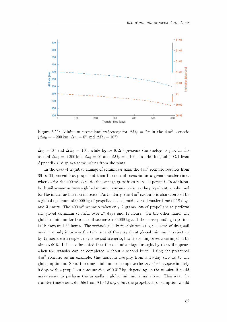
6.2. Minimum-propellant solutions
0 100 200 300 400 500 600
Transfer time [days]
100
150
200
250
300
350
400
450
500
550
600
Altitude [km
]
50.98
50.99
51
51.01
51.02
51.03
51.04
51.05
Inclin
ation [degre
es]
Figure 6.11: Minimum propellant trajectory for ∆Ωf = 2π in the 4 m2 scenario(∆a0 = +200 km, ∆ı0 = 0 and ∆Ω0 = 10)
∆ı0 = 0 and ∆Ω0 = 10, while gure 6.12b presents the analogous plot in the
case of ∆a0 = +200 km, ∆ı0 = 0 and ∆Ω0 = −10. In addition, table C.1 from
Appendix C displays some values from the plots.
In the case of negative change of semimajor axis, the 4 m2 scenario requires from
30 to 60 percent less propellant than the no sail scenario for a given transfer time,
whereas for the 400 m2 scenario the savings grow from 80 to 90 percent. In addition,
both sail scenarios have a global minimum around zero, as the propellant is only used
for the initial inclination increase. Particularly, the 4 m2 scenario is characterized by
a global optimum of 0.009 kg of propellant consumed over a transfer time of 18 days
and 3 hours. The 400 m2 scenario takes only 2 grams less of propellant to perform
the global optimum transfer over 17 days and 18 hours. On the other hand, the
global minimum for the no sail scenario is 0.069 kg and the corresponding trip time
is 18 days and 22 hours. The technologically feasible scenario, i.e. 4 m2 of drag sail
area, not only improves the trip time of the propellant global minimum trajectory
by 19 hours with respect to the no sail scenario, but it also improves consumption by
almost 90%. It has to be noted that the real advantage brought by the sail appears
when the transfer can be completed without a second burn. Using the presented
4 m2 scenario as an example, this happens roughly from a 17-day trip up to the
global optimum. Since the time minimum to complete the transfer is approximately
9 days with a propellant consumption of 0.317 kg, depending on the mission it could
make sense to perform the propellant global minimum maneuver. This way, the
transfer time would double from 9 to 18 days, but the propellant consumption would
87

6.2. Minimum-propellant solutions
6 8 10 12 14 16 18 20
Transfer time [days]
0
0.05
0.1
0.15
0.2
0.25
0.3
0.35P
rop
ella
nt
ma
ss [
kg
]
smax
= 0.04 m2
smax
= 4 m2
smax
= 400 m2
(a) ∆a0 = −200 km, ∆ı0 = 0 and ∆Ω0 = 10
12 14 16 18 20 22
Transfer time [days]
0.06
0.08
0.1
0.12
0.14
0.16
0.18
0.2
Pro
pe
llan
t m
ass [
kg
]
smax
= 0.04 m2
smax
= 4 m2
smax
= 400 m2
(b) ∆a0 = +200 km, ∆ı0 = 0 and ∆Ω0 = −10
Figure 6.12: Minimum-propellant as a function of transfer time
drop almost completely. This could be for example the case of an ADR mission,
which would require to collect as much debris as possible given a certain amount of
propellant.
Opposite conclusions can be drawn for the case of positive change of semimajor
axis. In fact, for both sail scenarios the performance improvement in terms of propel-
lant consumption decreases as the transfer time increases. Furthermore, the curves
converge to the same global optimum of 0.069 kg, as the corresponding solutions re-
quire the sail to be never deployed and the trajectories of all scenarios are identical.
Given a certain trip time, the propellant consumption improvement with respect to
the no sail scenario is around 10% in the 4 m2 scenario and reaches a maximum of
almost 40% in the 400 m2 scenario. Once again, depending on the mission it could
make sense to perform the global optimum trajectory, as for ADR. On the other
hand, for missions that require trade-os between transfer time and propellant con-
sumption, it has to be kept into account that the improvements brought by a drag
sail decrease as the trip time approaches the one of the global optimum trajectory.
This could be for example the case of on-orbit servicing.
Figure 6.13 highlights how increasing the maximum sail area value improves the
propellant consumption for a given trip time. Let us discuss the negative altitude
change rst (gure 6.13a). To begin with, the descent is aeroassisted and requires
less propellant. In addition, for higher values of Smax it can also be performed at a
faster rate. This means that the coasting arc can be extended over a longer period
of time, and moved at a lower altitude and at a lower inclination,. Consequently, the
rst and second burn are shorter. In the presented case, i.e. a 10-day trip, a S/C
equipped with a 4 m2 sail would deploy it before the second burn, while a 400 m2
value would be enough to not require a second burn at all.
As for the positive altitude change case, a 13-day trip is presented. In the 4 m2
scenario, the S/C initially res the thruster and deploys the sail at the same time.
88

6.2. Minimum-propellant solutions
0 2 4 6 8 10 12
Transfer time [days]
100
200
300
400
500
600
700
Altitu
de
[km
]
smax
= 0.04 m2
smax
= 4 m2
smax
= 400 m2
0 2 4 6 8 10 12
Transfer time [days]
51
51.02
51.04
51.06
51.08
51.1
51.12
Inclin
atio
n [
de
gre
es]
smax
= 0.04 m2
smax
= 4 m2
smax
= 400 m2
(a) ∆a0 = −200 km, ∆ı0 = 0 and ∆Ω0 = 10
0 2 4 6 8 10 12 14
Transfer time [days]
100
200
300
400
500
600
700
Altitu
de
[km
]
smax
= 0.04 m2
smax
= 4 m2
smax
= 400 m2
0 2 4 6 8 10 12 14
Transfer time [days]
50.93
50.94
50.95
50.96
50.97
50.98
50.99
51
Inclin
atio
n [
de
gre
es]
smax
= 0.04 m2
smax
= 4 m2
smax
= 400 m2
(b) ∆a0 = +200 km, ∆ı0 = 0 and ∆Ω0 = −10
Figure 6.13: Minimum-propellant trajectories for a given trip time
89

6.2. Minimum-propellant solutions
The descent is similar to that of the no-sail scenario; however, the S/C turns o
the thruster at an earlier time and at a higher altitude. Nevertheless, the descent
is continued to a lower altitude and the sail is then furled. Although the second
burn is longer, the propellant saved during the descent results in an overall lower
expenditure. Interestingly, in the 400 m2 scenario the initial descent is performed
without the use of thrust and the S/C coasts at approximately the same altitude of
the no sail scenario. Since there's no initial burn and the nal one takes roughly the
same amount of time, the propellant consumption is null for the rst and just about
the same for the latter.
Let us now study the case of orbits with lines of nodes initially drifting apart.
Figure 6.14 presents the propellant consumption for the three scenarios as a function
of transfer time, in the case of ∆a0 = +200 km, ∆ı0 = 0 and ∆Ω0 = 10. The
faint aerodynamic eects at the altitudes of the transfer and the brief time over
which the descent is performed result in modest improvement of the two drag sails
scenarios. For trip times under 100 days (gure 6.14a) small improvements can be
seen only for the 400 m2 scenario, whereas the 4 m2 is almost identical to the no sail
scenario. The trajectories for a trip time of 30 days and for a trip time of 40 days
are shown in gure 6.15. While the trajectory for the rst two scenarios is almost
the same, the 400 m2 value is large enough to be briey exploited during the nal
descent; the inclination of the waiting orbit can be slightly lower and the altitude
slightly higher. For the 30-day transfer the second burn is somewhat shorter, while
the 40-day maneuver is long enough to perform the descent without the use of thrust.
For trip times from 100 to 350 days (gure 6.14b) the 4 m2 scenario goes from being
similar to the no-sail scenario to being almost equivalent to the 400 m2 scenario. In
fact, as the trip time increases, the orbital decay in the 4 m2 scenario becomes more
and more pronounced than that of the no-sail scenario. The second burn can then
be slightly shorter, analogously to the 30-day trip in the 400 m2 scenario. For even
longer transfers (over 200 days), the second burn disappears in the 4 m2 scenario
as well. However, the semimajor axis decrease happens at a much slower rate than
that of the 400 m2 scenario. As a consequence, the S/C spends more time at lower
altitudes, where the eect of J2 is higher. In order to account for this, the waiting
orbit is higher, hence the dierence of propellant consumption. For trip times over
350 days the descents of the two drag sail scenarios become very brief and similar,
and so does the propellant expenditure. From a certain point on, the curves begin
to converge at the global optimum of 0.069 kg, common to all three cases since the
trajectory doesn't require the deployment of the sail. Table C.2 from Appendix C
shows the results in detail.
It has to be noted that even for long mission such as ADR, a single debris to debris
transfer can't be extended over prohibitively long times; an acceptable transfer could
be in the order of 60 days. In the case presented, having a 4 m2 drag sail would be
90

6.2. Minimum-propellant solutions
20 40 60 80 100
Transfer time [days]
0.1
0.2
0.3
0.4
0.5
Pro
pe
llan
t m
ass [
kg
]
smax
= 0.04 m2
smax
= 4 m2
smax
= 400 m2
(a) Detail from minimum-time to 100 days
100 150 200 250 300 350
Transfer time [days]
0.07
0.075
0.08
0.085
0.09
0.095
0.1
Pro
pe
llan
t m
ass [
kg
]
smax
= 0.04 m2
smax
= 4 m2
smax
= 400 m2
(b) Detail from 100 to 350 days
Figure 6.14: Minimum-propellant as a function of transfer time (∆a0 = +200 km,∆ı0 = 0 and ∆Ω0 = 10)
0 5 10 15 20 25 30 35 40
Transfer time [days]
400
500
600
700
800
Altitu
de
[km
]
smax
= 0.04 m 2
smax
= 4 m 2
smax
= 400 m 2
0 5 10 15 20 25 30 35 40
Transfer time [days]
400
500
600
700
800
Altitu
de
[km
]
smax
= 0.04 m 2
smax
= 4 m 2
smax
= 400 m 2
Figure 6.15: Minimum-propellant trajectories for trip times of 30 and 40 days (∆a0 =+200 km, ∆ı0 = 0 and ∆Ω0 = 10)
91

6.2. Minimum-propellant solutions
almost completely useless for such trip time. However, the propellant consumption
improvement highly depends on the initial and nal orbit, as ying through thicker
density values enhances the aeroassisted maneuvers. As a general trend, in the case
positive altitude change transfers, the use of drag sails is benecial when the line of
nodes of the target orbit is initially moving closer to the one of the chaser or, when the
lines of nodes are drifting apart, if the transfer is performed between orbits below
400 km of altitude. On the other hand, it has been shown that negative altitude
change transfers can be carried out with nearly-zero-consumption maneuvers. As for
minimum-time trajectories, negative altitude change transfers are improved by a few
hours when a 4 m2 drag sail is employed and by a a few days when Smax = 400 m2. In
addition, increasing the maximum frontal area doesn't improve the minimum time
of positive altitude change transfers by much. In light of this, the use of a drag
sail wouldn't make much sense for missions that require the S/C to reach the target
orbit as fast as possible (e.g. a satellite that must reach its operative orbit). As a
matter of fact, even a light sail would take a toll on the cost of the mission and, at
the same time, take up some volume and mass that would be otherwise assigned to
other subsystems. On the ip side, OOS and ADR missions could exploit drag sails
to a much greater extent. Even though the scope of this thesis was not to give a
direct example of such missions, the results obtained show that a drag-enhancement
system should be investigated during mission analysis.
92

Conclusions
The optimization of space trajectories in low Earth orbit is becoming of extreme
interest due to several new mission concepts, such as active debris removal, on-orbit
servicing and small-sat deployment from orbiting platforms. This thesis provides a
fast and accurate method for the evalutation of these transfers. In particular, the
eects of the Earth's gravitational harmonic J2 coecient and aerodynamic drag are
kept into account in order to obtain meaningful results.
After showing how to build a mathematical model to approximate the afore-
mentioned perturbations, an indirect optimization approach has been applied. This
method transforms the optimization problem into a boundary value problem, which
is solved by means of shooting procedures. The use of drag sails is investigated by
treating the frontal area of the spacecraft as a control variable, in addition to thrust
magnitude and direction. The analysis of a case study has displayed the structure of
the solutions to the minimum-time and minimum-propellant problems. Depending
on the parameters that dene the transfer, i.e. relative orbital elements and available
trip time, the enhancement of aerodynamic drag may be highly benecial in terms
of propellant expenditure. On the ip side, time of ight is improved signicantly
only for relatively large values of maximum frontal area. Therefore, this thesis oers
a framework for fast trade-o studies on the use of drag sails for future missions.
Although the atmospheric model used in this work is not particularly accurate,
the method proposed is readily extendible to deal with more sophisticated models.
Proper phasing of the chaser spacecraft to rendezvous with the target has not been
accounted for. Moreover, the changes of semimajor axis and inclination of the target
have been neglected, as the case study assumed it performed maneuvers in opposition
to the eects of aerodynamic drag. In light of this, future studies may use the
described method to dene optimal strategies for a specic active debris removal or
on-orbit servicing mission. A more detailed atmospheric model may be easily plugged
in and the rendezvous phase may be accounted for. Finally, further complexity may
be added by removing the almost-circular orbit approximation and considering the
eccentricity equation and the eect of J2 on the line of apses.
93

Bibliography
[1] Roger R Bate, Donald D Mueller, Jerry E White, and William W Saylor. Fun-
damentals of astrodynamics. Courier Dover Publications, 2020.
[2] Bruce Bowman, W. Kent Tobiska, Frank Marcos, Cheryl Huang, Chin Lin, and
William Burke. A New Empirical Thermospheric Density Model JB2008 Using
New Solar and Geomagnetic Indices.
[3] Arthur Earl Bryson. Applied optimal control: optimization, estimation and
control. CRC Press, 1975.
[4] Lorenzo Casalino and Guido Colasurdo. Improved Edelbaum's Approach to Op-
timize LEO-GEO Low-Thrust Transfers.
[5] Guido Colasurdo and Lorenzo Casalino. Indirect Methods for the Optimization
of Spacecraft Trajectories, pages 141158. Springer New York, New York, NY,
2013.
[6] Guido Colasurdo and Lorenzo Casalino. Tentative Solutions for Indirect Opti-
mization of Spacecraft Trajectories, pages 87102. Springer International Pub-
lishing, Cham, 2016.
[7] Bruce A. Conway. The Problem of Spacecraft Trajectory Optimization, pages
115. Cambridge Aerospace Series. Cambridge University Press, 2010.
[8] Theodore N. Edelbaum. Propulsion requirements for controllable satellites. ARS
Journal, 31(8):10791089, 1961.
[9] Theodore N. Edelbaum. Theory of maxima and minima. In George Leitmann,
editor, Optimization Techniques, volume 5 of Mathematics in Science and En-
gineering, pages 132. Elsevier, 1962.
[10] L. Johnson, D. Alhorn, Mark Boudreaux, J. Casas, D. Stetson, and R. Young.
Solar and drag sail propulsion: From theory to mission implementation. 2014.
[11] Jean A. Kechichian. Optimal altitude-constrained low-thrust transfer between
inclined circular orbits. The Journal of the Astronautical Sciences, 54(3):485
503, December 2006.
94

Bibliography
[12] Jean A. Kechichian. Optimal low-thrust transfer in general circular orbit using
analytic averaging of the system dynamics. The Journal of the Astronautical
Sciences, 57(1):369392, January 2009.
[13] Jean Albert Kechichian. Reformulation of edelbaum's low-thrust transfer prob-
lem using optimal control theory. Journal of Guidance, Control, and Dynamics,
20(5):988994, 1997.
[14] Donald J. Kessler and Burton G. Cour-Palais. Collision frequency of articial
satellites: The creation of a debris belt. Journal of Geophysical Research: Space
Physics, 83(A6):26372646, 1978.
[15] Donald E Kirk. Optimal control theory: an introduction. Courier Corporation,
2004.
[16] Louis Komzsik. Applied calculus of variations for engineers. CRC Press, 2019.
[17] Joerg Kreisel. On-orbit servicing (oos): Issues & commercial implications. 09
2003.
[18] Dazhong Lao and Shanshan Zhao. Fundamental Theories and Their Applica-
tions of the Calculus of Variations. Springer, 2020.
[19] J.-C. Liou and N. L. Johnson. Risks in space from orbiting debris. Science,
311(5759):340341, 2006.
[20] United States. National Oceanic, Atmospheric Administration, and United
States. Air Force. US standard atmosphere, 1976, volume 76. National Oceanic
and Atmospheric Administration, 1976.
[21] L.F. Shampine, M.K. Gordon, L.F. Gordon, M.K. Gordon, W. H. Freeman, and
Company. Computer Solution of Ordinary Dierential Equations: The Initial
Value Problem. W. H. Freeman, 1975.
[22] Daniel Tabak. Introduction to control theory including optimal control, d. n.
burghes and a. graham, ellis horwood ltd. Optimal Control Applications and
Methods, 2(2):203204, 1981.
[23] Andrew Tatsch, Norman Fitz-Coy, and Svetlana Gladun. On-orbit servicing:
A brief survey. In Proceedings of the IEEE International Workshop on Safety,
Security, and Rescue Robotics, pages 276281, 2006.
[24] Craig Underwood, Andrew Viquerat, Mark Schenk, Ben Taylor, Chiara Mas-
simiani, Richard Duke, Brian Stewart, Simon Fellowes, Chris Bridges, Guglielmo
Aglietti, Berry Sanders, Davide Masutti, and Amandine Denis. Inatesail de-
orbit ight demonstration results and follow-on drag-sail applications. Acta
Astronautica, 162:344358, 2019.
95

Bibliography
[25] David A Vallado. Fundamentals of astrodynamics and applications, volume 12,
chapter 8, pages 559569. Springer Science & Business Media, 2001.
[26] Ting Wang. Analysis of debris from the collision of the cosmos 2251 and the
iridium 33 satellites. Science & Global Security, 18(2):87118, 2010.
[27] William E. Wiesel and Salvatore Alfano. Optimal many-revolution orbit trans-
fer. Journal of Guidance, Control, and Dynamics, 8(1):155157, 1985.
96

Appendix A
Vector and matrix operations
This appendix lists useful vector and matrix operations that will be used in this
thesis.
A.1 Vector operations
Scalar product The scalar product of two vectors a and b, denoted by a · b, isdened as
a · b = ab cosϑ (A.1)
where ϑ is the angle between the two vectors. Following this denition, one has
a · b = b · a (A.2)
a · (b + c) = a · b + a · c (A.3)
α (a · b) = αa · b = a · αb (A.4)
a · a = a2 (A.5)
a · a = aa (A.6)
If i, j and k are unit orthogonal vectors, a = a1i + a2j + a3k and b = b1i + b2j + b3k,
one has
i · j = j · k = i · k = 0 (A.7)
a · b = (a1i + a2j + a3k) · (b1i + b2j + b3k) (A.8)
Using equations (A.3) and (A.7), equation (A.8) rewrites as
a · b = a1b1 + a2b2 + a3b3 (A.9)
97

A.2. Vector notation
Vector product The vector product of two vectors a and b, denoted by a× b, is
a vector c such that
c = ab sinϑ (A.10)
where ϑ is the angle between the two vectors and its direction is perpendicular to
both a and b. Following this denition, one has
a× b =
∣∣∣∣∣∣∣i j k
a1 a2 a3
b1 b2 b3
∣∣∣∣∣∣∣ = det
i j k
a1 a2 a3
b1 b2 b3
(A.11)
whete i, j and k are unit orthogonal vectors, a = a1i+a2j+a3k and b = b1i+b2j+b3k.
In addition,
a× a = 0 (A.12)
a× b = − (b× a) (A.13)
a× (b + c) = a× b + a× c (A.14)
α (a× b) = αa× b = a× αb (A.15)
a× (b× c) = (a · c) b− (a · b) c (A.16)
(a× b)× c = (a · c) b− (b · c) a (A.17)
a · (b× c) = c · (a× b) = b · (c× a) (A.18)
Equation (A.18) is readily proved by expanding equation (A.18) by using equations
(A.11) and (A.9), which give∣∣∣∣∣∣∣a1 a2 a3
b1 b2 b3
c1 c2 c3
∣∣∣∣∣∣∣ =
∣∣∣∣∣∣∣c1 c2 c3
a1 a2 a3
b1 b2 b3
∣∣∣∣∣∣∣ =
∣∣∣∣∣∣∣b1 b2 b3
c1 c2 c3
a1 a2 a3
∣∣∣∣∣∣∣which is easy to verify.
A.2 Vector notation
This work assumes a bold character denotes a column vector:
a =
a1
a2
...
an
(A.19)
98

A.2. Vector notation
A row vector is written as aT , where the letter T denotes the transpose matrix. This
way, the scalar product a · b can be written as
a · b = aTb = bTa (A.20)
The time derivative of a column vector yields a column vector whose components
are the time derivatives of each one of the components of the vector:
da
dt=
da1/dt
da2/dt...
dan/dt
(A.21)
The derivative of a scalar quantity with respect to a column vector yields a row
vector whose components are the derivatives of the scalar quantity with respect to
the components of the vector:
dϕ
da=
(dϕ
da1,dϕ
da2, . . . ,
dϕ
dan
)The derivative of a vector a with n components with respect to another vector b with
m components yields a matrix with n rows and m columns. Each column containes
the derivatives of the components of a with respect to a single component of b,
whereas each row containes the derivatives of a single components of a with respect
to the components of b:
[da
db
]=
da1/db1 · · · da1/dbm
.... . .
...
dan/db1 · · · dan/dbm
99

Appendix B
Coordinate transformations
A physical vector is a mathematical quantity that has three dimensions and only
possesses two properties: magnitude and direction. The concept of physical vector
and all of the operations associated with physical vectors are completely indipendent
of a coordinate system. However, frames of reference are needed for the formulation of
kinematics and dynamics. The same physical vector can be expressed in any suitable
coordinate system. In the case of rectangular coordinate systems, any physical vector
can be expressed as a linear combination of the three unit vectors that make up the
basis of the system. Given a coordinate system, a coordinate transformation only
changes the basis of a vector. That mathematical properties that dene the vector
(magnitude and direction) remain unchanged.
Rotation matrices Suppose we have the coordinates of a vector in a certain
coordinate system XYZ
a = aXX + aY Y + aZZ
and we want to calculate its coordinates in another system UVW
a = aUU + aV V + aWW
The coordinates are simply given by
aU = a ·U
aV = a ·V
aW = a ·W
100

Therefore, by using equations (A.3) and (A.4) we can write
aU = aX (X ·U) + aY (Y ·U) + aZ (Z ·U)
aV = aX (X ·V) + aY (Y ·V) + aZ (Z ·V) (B.1)
aW = aX (X ·W) + aY (Y ·W) + aZ (Z ·W)
By using the notation introduced in Appendix A, we can write
aUVW =
aU
aV
aW
aXY Z =
aX
aY
aZ
where the subscripts identify the coordinate system. By introducing the rotation
matrix
L =
X ·U Y ·U Z ·UX ·V Y ·V Z ·VX ·W Y ·W Z ·W
(B.2)
we can write
aUVW = LaXY Z (B.3)
which, by applying the rules of matrix multiplication, yields the set of equations
(B.1).
The columns of matrix (B.2) are the unit vectos of XYZ expressed in UVW:
L =[
XUVW YUVW ZUVW
]The multiplication between the transpose of L and itself yields
LT · L =
XTUVW
YTUVW
ZTUVW
[ XUVW YUVW ZUVW
]=
=
1 0 0
0 1 0
0 0 1
This shows that L−1 = LT and the rotation matrix is an orthonormal matrix. This
101

implies that we can invert the transformation in equation (B.3) and write
aXY Z = LTaUVW
Let us now consider three coordinate systems, denoted as 1, 2 and 3. Let L21
be the rotation matrix from coordinate system 1 to 2 and L32 the transformation
matrix from 2 to 3. Therefore, we can write
a3 = L32a2 = L32L21a1
If L31 is the rotation matrix from coordinate system 1 to 3, we have
L31 = L32L21 (B.4)
Therefore, successive rotations can be combined to transform the coordinates of a
vector.
Principal rotations If two coordinate systems are related by a simple rotation
through a positive angle α about an axis, the rotation matrix assumes a simple
form. Let us assume coordinate system UVW is obtained by rotating XYZ through
an angle α about the Z-axis, such that Z ≡W. The rotation matrix from equation
(B.2) becomes
L =
cosα sinα 0
− sinα cosα 0
0 0 1
In the same manner, for a rotation about the Y-axis,
L =
cosα 0 − sinα
0 1 0
sinα 0 cosα
whereas for a rotation about the X-axis,
L =
1 0 0
0 cosα sinα
0 − sinα cosα
Transformation from the Geocentric-Equatorial to the Perifocal coordi-
nate system The perifocal coordinate system can be obtained from the geocentric-
equatorial system through successive rotations. As a matter of fact, by rotating IJK
through an angle equalt to the RAAN Ω about K, the transformed x-axis lies along
the line of nodes. A further rotation through the inclination angle ı about the new
102

x-axis, transforms the z-axis in w (the z-axis of the perifocal frame). Finally, a ro-
tation through an angle equal to the argument of perigee ω about w completes the
transformation. By applying the rule of successive rotations as described by equation
(B.4), we have
LpqwIJK =
cosω sinω 0
− sinω cosω 0
0 0 1
1 0 0
0 cos ı sin ı
0 − sin ı cos ı
cos Ω sin Ω 0
− sin Ω cos Ω 0
0 0 1
Multiplicating the matrixes yields
LpqwIJK = cos Ω cosω − sin Ω sinω cos ı sin Ω cosω + cos Ω sinω cos ı sinω sin ı
− cos Ω sinω − sin Ω cosω cos ı − sin Ω sinω + cos Ω cosω cos ı cosω sin ı
sin Ω sin ı − cos Ω sin ı cos ı
(B.5)
Therefore, we have
apqw = LpqwIJKaIJK (B.6)
and
aIJK = LTpqwIJKapqw (B.7)
Transformation from the Perifocal to the RTW coordinate system As
described in Section 2.4.1.1, the RTW coordinate system is the rotation of the peri-
focal coordinate system through an angle equal to the true anomaly ν about w. The
rotation matrix is
LRTWpqw =
cos ν sin ν 0
− sin ν cos ν 0
0 0 1
(B.8)
103

Appendix C
Minimum-propellant tables
Table C.1: Minimum propellant consumption for transfer with lines of nodes initiallymoving closer
∆a0 = −200 km∆ı0 = 0°
∆Ω0 = 10°
∆a0 = +200 km∆ı0 = 0°
∆Ω0 = −10°
No dragsail
Smax =4 m2
Smax =400 m2
No dragsail
Smax =4 m2
Smax =400 m2
tf [days] mp [kg]
12 0.183 0.134 0.039 0.198 0.184 0.12612.5 0.167 0.121 0.034 0.183 0.164 0.12013 0.153 0.109 0.029 0.170 0.150 0.11413.5 0.141 0.098 0.025 0.158 0.139 0.10914 0.130 0.089 0.021 0.148 0.130 0.10414.5 0.121 0.080 0.018 0.138 0.122 0.10015 0.113 0.071 0.015 0.130 0.115 0.09615.5 0.105 0.063 0.012 0.123 0.108 0.09316 0.099 0.055 0.009 0.116 0.102 0.08916.5 0.092 0.046 0.007 0.110 0.096 0.08717 0.086 0.036 0.005 0.104 0.091 0.084
Global optimum 0.069 0.009 0.002 0.069 0.069 0.069
104

Table C.2: Minimum propellant consumption for transfer with lines of nodes initiallydrifting apart (∆a0 = +200 km, ∆ı0 = 0 and ∆Ω0 = 10)
No drag sail Smax = 4 m2 Smax = 400 m2
tf [days] mp [kg]
20 0.269 0.269 0.259
30 0.183 0.183 0.167
40 0.150 0.150 0.114
50 0.132 0.131 0.102
60 0.120 0.120 0.095
70 0.112 0.111 0.090
80 0.106 0.105 0.087
90 0.102 0.101 0.085
100 0.098 0.097 0.083
110 0.095 0.094 0.082
120 0.093 0.091 0.080
130 0.091 0.089 0.079
140 0.089 0.087 0.079
150 0.088 0.085 0.078
160 0.087 0.084 0.077
170 0.085 0.082 0.077
180 0.084 0.081 0.076
190 0.083 0.080 0.076
200 0.083 0.078 0.075
210 0.082 0.077 0.075
220 0.081 0.076 0.075
230 0.081 0.076 0.074
240 0.080 0.075 0.074
250 0.080 0.075 0.074
260 0.079 0.074 0.074
270 0.079 0.074 0.073
280 0.078 0.074 0.073
290 0.078 0.074 0.073
300 0.078 0.073 0.073
310 0.077 0.073 0.073
320 0.077 0.073 0.072
330 0.077 0.073 0.072
340 0.076 0.072 0.072
350 0.076 0.072 0.072
105

No drag sail Smax = 4 m2 Smax = 400 m2
tf [days] mp [kg]
360 0.076 0.072 0.072
370 0.076 0.072 0.072
380 0.075 0.072 0.072
390 0.075 0.072 0.072
400 0.075 0.072 0.072
410 0.075 0.072 0.071
420 0.075 0.072 0.071
430 0.075 0.071 0.071
440 0.074 0.071 0.071
450 0.074 0.071 0.071
460 0.074 0.071 0.071
470 0.074 0.071 0.071
480 0.074 0.071 0.071
490 0.074 0.071 0.071
500 0.074 0.071 0.071
510 0.073 0.071 0.071
520 0.073 0.071 0.071
530 0.073 0.071 0.071
540 0.073 0.071 0.071
550 0.073 0.071 0.071
560 0.073 0.071 0.071
570 0.073 0.071 0.070
580 0.073 0.070 0.070
590 0.073 0.070 0.070
600 0.073 0.070 0.070
610 0.072 0.070 0.070
620 0.072 0.070 0.070
630 0.072 0.070 0.070
640 0.072 0.070 0.070
650 0.072 0.070 0.070
660 0.072 0.070 0.070
670 0.072 0.070 0.070
680 0.072 0.070 0.070
690 0.072 0.070 0.070
700 0.072 0.070 0.070
710 0.072 0.070 0.070
Global optimum 0.069 0.069 0.069
106