optimal long-run option investment strategies
TRANSCRIPT
Optimal Long-Run Option Investment StrategiesAuthor(s): Richard J. Rendleman, Jr.Source: Financial Management, Vol. 10, No. 1 (Spring, 1981), pp. 61-76Published by: Wiley on behalf of the Financial Management Association InternationalStable URL: http://www.jstor.org/stable/3665114 .
Accessed: 16/06/2014 15:37
Your use of the JSTOR archive indicates your acceptance of the Terms & Conditions of Use, available at .http://www.jstor.org/page/info/about/policies/terms.jsp
.JSTOR is a not-for-profit service that helps scholars, researchers, and students discover, use, and build upon a wide range ofcontent in a trusted digital archive. We use information technology and tools to increase productivity and facilitate new formsof scholarship. For more information about JSTOR, please contact [email protected].
.
Wiley and Financial Management Association International are collaborating with JSTOR to digitize, preserveand extend access to Financial Management.
http://www.jstor.org
This content downloaded from 195.34.79.223 on Mon, 16 Jun 2014 15:37:40 PMAll use subject to JSTOR Terms and Conditions

Optimal Long-Run Option
Investment Strategies
Richard J. Rendleman, Jr.
The author is Associate Professor of Finance at The Fuqua School of Business at Duke University. He extends special thanks to the DePaul University College of Commerce for providing partial funding and computational assistance for his study.
Introduction
Recent theories of option pricing, such as the Black and Scholes (BS) option pricing model [1] and the work of Merton [12], have been based to a large extent on the idea that equilibrium option prices cannot provide investors with the ability to earn riskless ar- bitrage profits.1 If the no-arbitrage conditions under- lying the models are violated in practice, it may be possible for a trader who faces low trading costs to earn riskless excess returns.2
'Under the BS model, the price of the underlying stock is assumed to follow a random walk described by a lognormal distribution. Under this assumption, if investors can trade options and stock with no transaction costs, it is possible to form a riskless hedge that in- volves a continuously revised position in the option and its under- lying stock. The BS model determines the price for which such a hedge yields the riskless rate of interest. If the option is not priced according to the model, the type of continuously revised riskless hedge described by BS will enable the investor to earn a riskless ar- bitrage profit. Using a discrete multiplicative binomial distribution which can approximate a lognormal distribution, Cox, Ross, and Rubinstein [4] provide an excellent exposition on the mechanics of this type of riskless arbitrage.
Most normative option trading models are based on an objective of earning riskless arbitrage returns. (See, for example, Black and Scholes [2], Latane and Rendleman [11], Chiras and Manaster [3], Schmalensee and Trippi [14], Trippi [16], Galai [6, 7], Gould and Galai [8], and Klemkosky and Resnick [10].) Although these normative models have been employed extensively by individuals and institutions that make a market in listed options, they cannot be used as effectively by investors who are unable to trade at a low cost or who do not have the time or the resources to monitor the options and stock markets on an ongoing basis. There are many practical option in- vestment strategies, however, that can effectively be used that do not involve the riskless arbitrage concept at all.
2In addition to brokerage commissions, the arbitrageur must con- sider the costs associated with the bid-asked spread in any options and stock in which he is dealing as well as the cost of carrying a short position. In many cases, these costs will more than offset any potential riskless arbitrage returns.
61
This content downloaded from 195.34.79.223 on Mon, 16 Jun 2014 15:37:40 PMAll use subject to JSTOR Terms and Conditions
FINANCIAL MANAGEMENT/SPRING 1981
A portfolio strategy that is based on holding risky option positions to maturity along with the under- lying stocks and/or safe assets is likely to be more relevant for individuals and institutions that use op- tions as a form of investment rather than as a vehicle for riskless hedging or speculation. The purpose of this
paper is to examine the optimal security mix for a
portfolio consisting of a single stock, a call option on the stock, and a safe asset. It is assumed that the port- folio is held without revision until the option's maturity date, and various assumptions are made about the option's price, the expected return and risk characteristics of the stock, and the utility function of the investor. The analysis should provide the reader with some practical insights into the use of options as a means of improving a stock portfolio's long-run per- formance.
To my knowledge, the only published work that is similar to the present study is that of Merton, Scholes, and Gladstein [13], who examined the historical risk and return characteristics of fully covered call option writing positions and portfolios consisting of 10% call
options and 90% commercial paper. The study used actual stock price data for the period July 1963
through December 1975, but option prices were simulated using the BS model, as listed options were not traded over much of the sample period. In contrast to the present study, Merton, Scholes, and Gladstein made no attempt to determine the optimal security mix.
The Objective Function
A generalized isoelastic (power) utility function is used as a basis for determining optimal portfolio policy. The isoelastic utility function possesses the following properties which make it particularly attrac- tive in portfolio selection.
1. The optimal proportion of portfolio funds to in- vest in a given security is independent of the in- vestor's wealth level.
2. Present investment decisions can be made without regard to future investment decisions.
3. No portfolio will be selected that offers a
positive probability of ruin.3 Letting ft represent the portfolio's return per dollar
invested (one plus the return), the generalized iso- elastic utility function takes the following form:4
8This can be seen by evaluating Equation (1) below as f approaches zero. In such cases, the portfolio's expected utility will approach negative infinity even if the probability of such an outcome is small.
E(U(H)) = E( l-
1). l-y
(1)
E(.) is the expectation operator, and y represents the investor's coefficient of relative risk aversion. The coefficient is a measure of the investor's willingness to take risks of a given size relative to his wealth. Assum-
ing risk averse behavior, y must be greater than zero, and larger values of y indicate greater aversion to risk.
Unfortunately, I cannot provide any guidance on the proper utility function to use in evaluating option portfolios. Two special cases, though, may provide points of reference.
If y equals zero, the investor is risk neutral and will select the portfolio with the highest expected return
regardless of its risk. If y equals one, the investor has a
logarithmic utility function. [Technically, the limit of
U(H) as y approaches 1 is ln(H) in Equation (1).] A
logarithmic utility maximizer will select the portfolio with the highest expected continuously compounded rate of return (growth rate). Such an investor does not care about the uncertainty surrounding the expected continuous return. Investors who are risk averse but less risk averse than the logarithmic utility maximizer would have a coefficient of relative risk aversion that is greater than zero but less than one. Finally, the coefficient of relative risk aversion would be greater than one for an investor who is more risk averse than the logarithmic utility maximizer.
Elton and Gruber [5] have shown that the optimal portfolio mix will be the same for both the long-run and short-run investor only when an isoelastic utility function characterizes investor behavior. Thus, an in- vestor who desires to spend all wealth on consumption goods when the option matures will select the same
portfolio as an investor who may have a longer-run consumption horizon in mind.
Assumptions
Although some simplifying assumptions must be made to make the problem of selecting an optimal stock-option-safe asset portfolio mathematically trac- table, none which is made in this analysis is terribly unrealistic. Except for the noncontinuous nature of the investor's holding period, all the assumptions are com- mon throughout the option pricing literature.
1. The returns per dollar invested in the underlying
4Technically, optimal portfolio compositions would be identical to those based on Equation (1) if the following simpler version of Equation (I) were used: E(U[H]) = E(HI-Y). However, the form in Equation (1) is chosen so that U(H) = ln(l) as y approaches 1.
62
This content downloaded from 195.34.79.223 on Mon, 16 Jun 2014 15:37:40 PMAll use subject to JSTOR Terms and Conditions

RENDLEMAN/OPTION INVESTMENT STRATEGIES
stock follow a random walk described by a log- normal distribution with a geometric drift (ex- pected logarithmic return or growth rate) of , and variance, oa, per unit of time.
2. Investors can borrow or lend at the same rate of interest.5
3. The underlying stock is expected to pay no dividends or any other monetary distributions throughout the life of the option.
4. There are no transaction costs, taxes, or restric- tions on short sales involved with the purchase or sale of any security.
5. All option positions are maintained until the op- tion's maturity date.
In the analysis, optimal portfolio compositions are determined for options that are priced according to the BS model as well as for options that are both under- and overpriced relative to the model.
The Stock-Option-Safe Asset Portfolio Selection Model
In evaluating the expected utility from a portfolio that consists of an option, its underlying stock, and a safe asset, the investor must first estimate the returns per dollar invested in the three securities. Let fH, Hw, and Hf represent the returns per dollar invested in the stock, option, and safe asset, respectively, and q8, qw, and (1 - q, - qw) denote the portfolio proportions held in each of the three respective securities. Then, the portfolio's holding period return can be stated as:
fl = qeFs, + qwtw + (1 - q, - qw) H,.
The return per dollar invested in the safe asse assumed to be
Hf = er,
where r is the continuously compounded rate of terest to be earned over the option's life. Under assumption that the returns per dollar invested in underlying stock follow a lognormal distribution, stock's holding period return can be stated as:
8 = e
In Equation (4), u denotes the expected logarithi
SAlthough this appears to be a restrictive assumption, a policy of borrowing to fund a portfolio that has a finite probability of attain- ing a zero value will never serve as an optimal policy for isoelastic utility maximizers.
(2)
return or growth rate of the stock over the option's life, a is the standard deviation of the natural logarithm of the stock's holding period return over the option's life, and z denotes a standard normal random variable with a mean of zero and a standard deviation of one.
The option's holding period return will depend upon whether the option expires in or out of the money. If the option expires out of the money, the option's holding period return is zero. Otherwise the holding period return is equal to the option's maturity value (stock price at maturity minus the striking price) divided by the initial purchase price of the option. Denoting the current stock price as S, the value of the stock at maturity is SfH = Se . Subtracting the op- tion's striking price, X, from the maturity value of the stock and dividing the difference by the current option price, W, the in-the-money option holding period return is (Se'+" - X)/W. The option will be in the money when the maturity value of the stock is greater than the option's striking price, or when Se^" > X. This will occur when z > In(X/S) - P. Therefore, the option's holding period return can be stated as
Hf= (Se~+z- X)/W if > n(/S)-
=0 if z< ln(X/S) -. a
(5)
By substituting the returns per dollar invested from Equations (3) through (5) into Equation (2), the port- folio's holding period return becomes
Rf = qse+" + q,(Se"'+"- X)/W + (1 - q - qw)er
if > ln(X/S) - a
= q,e '++ (1 - q - qw)er
ifZ ln(X/S)-# (6)
The portfolio's expected utility can be computed by the substituting the portfolio holding period return from
Equation (6) into the utility function stated in Equa- tion (1), while recognizing that the normal probability
eQ?l (4) function is e . After making this substitution, the
mic portfolio's expected utility becomes
o0 B E(U(z)) = fi(zf) dz + f f2(Z) dz,
B-ao (7)
63
This content downloaded from 195.34.79.223 on Mon, 16 Jun 2014 15:37:40 PMAll use subject to JSTOR Terms and Conditions
FINANCIAL MANAGEMENT/SPRING 1981
where B = ln(X/S)- a
f () =([qseM+e + qw(Se"'"- X)/W +
(1 -y) v'2-
(1 - q8 - q)er]l-Y- l)e-'i'
(1 - y) V/2
= ([qse +
+ (1 -q q qw)er]I-y - 1)e-'^' (-- y)v-
The first integral in Equation (7) represents the port- folio's expected utility when the option expires in the money, and the second integral represents the port- folio's expected utility when the option expires worth- less.
The portfolio proportions that maximize the inves- tor's expected utility are found at the point where the partial derivatives of Equation (7) with respect to qs and qw are simultaneously set to zero (assuming that the second order conditions for a maximum are satis- fied). As noted below, the first order conditions for a maximum cannot be determined analytically, making it impossible to determine whether the second order conditions are also satisfied. However, by directly evaluating Equation (7) for a large number of values of q8 and qw, I am satisfied that the portfolio selection algorithm does in fact find the optimal solution.
The partial derivatives of Equation (7) with respect to qs and qw are given by the left-hand sides of Equa- tions (8A) and (8B), respectively. The optimal port- folio composition is found by determining the values of q8 and qw that simultaneously set the two partial derivatives to zero. Given a pair of optimal values of q, and qw, Equation (7) can be solved in terms of these values to determine the expected utility of the optimal portfolio.
co B
J f3(2)dZ + f4(2)d = 0 B -co
co B f f5(2)d2 + f f6(z)dz = 0 B -0o
where
f3(2) = (qe M+Gz + qw(Se+ - X)/W + (I - qs- qw)er).-Y (e +or - er) e-''P/2x/~,
(8a)
(8b)
f4(z) = (q,e+i+ (1 q - q- )er).Y (el+"z - er)e- /;/
f5(z) = (qseM+* + qw(Se`+i'- X)/W + (l - qs- qw)e r)- ((Se+' - X)/W - er)e-'h'/2
f6(z) = (q8e + + (1 - q8 - qw)er) ( r- e 1/22)/2
In a portfolio selection problem of this type in which the possibility for intertemporal trading is not considered, the optimal values of q8 and qw will always fall between certain bounds, even though restrictions are not explicitly placed on the portfolio. These im- plicit restrictions prevent the risk of ruin, which im- plies an expected utility level of -o.
If the investor borrows money to fund long posi- tions in both the option and stock, there is a possibil- ity that the stock price will fall to a point at which the investor cannot meet his debt obligation. Therefore, the first restriction prevents the possibility of ruin that can result if long positions in options and stock are partially funded through borrowing:
If q 2> 0 then qw < (1 - q,). (R1)
The second restriction ensures that every short posi- tion in either options or stock is at least fully covered by an equivalent long position in the other security:
For all q8, qw > -qs W/S. (R2)
The third restriction prevents the possibility of shorting stock and using the proceeds of the short sale to fund an option position that could result in a negative wealth level if the stock rises in value but the option expires worthless. In effect, this restriction prevents the possibility of ruin at stock prices at or below the option's striking price, assuming a short position is taken in the stock:
If qs < 0, then qw < (1 - qs) + q8XerS. (R3)
Finally, restrictions are placed on feasible values for q, so that the maximum value of qw, given a value of q., is never less than the minimum feasible value of qw:
qs < 1/(1 - W/S),
qs ? 1/(1 - Xe-r/S - W/S).
(R4)
(R5)
The fourth restriction combines R1 and R2. The only way that both conditions can be satisfied simulta-
64
This content downloaded from 195.34.79.223 on Mon, 16 Jun 2014 15:37:40 PMAll use subject to JSTOR Terms and Conditions
RENDLEMAN/OPTION INVESTMENT STRATEGIES
neously is if restriction R4 is met. The fifth condition combines R2 and R3, determining the values for q8 for which both R2 and R3 are simultaneously satisfied.6
Unfortunately, closed form solutions are not ob- tainable for any of the integrals in Equations (7), (8a), and (8b). As a result, optimal portfolio weights can- not be determined directly, and numerical analysis must be used to evaluate the integrals and to deter- mine optimal solutions. The procedure that is employed to evaluate these integrals and to solve for optimal portfolio weights is described in Appendix A.
Optimal Portfolio Compositions The optimal portfolio policy will depend upon the
expected growth rate and variance of returns of the underlying stock as well as the price of the option and the riskless interest rate. Before attempting to quan- tify these relationships, it is useful to review the economic principles which serve as the basis for the derivation of the BS model. These principles will provide a clue to the optimal portfolio composition in a limited number of cases, even before the problem is actually solved.
If options are priced according to the BS model, a continuously rebalanced stock-option portfolio can be made a perfect substitute for an investment in a riskless bond. In fact, at the BS price, it is possible to form a continuously rebalanced portfolio consisting of any two of the three securities which offers returns equivalent to those of the other security.
This perfect substitutability implies that if an option is priced according to the BS model, the option will not enable the investor to increase the expected utility of a continuously revised portfolio over that which can be attained with the stock and safe assets alone. The option would simply represent a redundant security that provides no additional investment opportunities for the continuous time trader. (Actually, any one of the three securities is redundant in terms of the other two when continuous revision is considered.) However, if the investor's trading horizon goes beyond the point at which the perfect substitutability among the securities can be maintained, options will expand the investor's return opportunities. In this situation, it is possible that options might enter the optimal solu- tion to the portfolio selection problem, even at the BS price.
6The reader should note that if the option is properly priced, W will exceed S - Xe-r [see Merton (12)]. As a result, the term (1 - Xe-r/S - W/S) will be negative. If the negative sign of this term is not recognized, one will reverse the sign of the inequality in R5 by mis- take.
The noncontinuous portfolio selection problem can be viewed as a constrained version of the continuous time problem, because the number of trades is limited. For example, an optimal solution to the continuous time problem that calls for always holding 50% of the portfolio in stock and 50% in bonds would not be a feasible solution to the noncontinuous problem, as the investor would have no control over the portfolio between trades.
There are two important situations in which the op- timal solution to the continuous time problem is a feasible solution to the noncontinuous problem, regardless of the trading interval. These solutions must, therefore, represent optimal solutions to the noncontinuous problem as well. The situations are summarized below, and the mathematics underlying the relationships is provided in Appendix B.
1. Assuming that an option is priced according to the BS model, an all-stock portfolio will be optimal when choosing among a stock, an option, and a safe asset, regardless of the investor's trading interval, if:
I = (y - 1/2) a2 + r (9)
For example, consider a stock with an expected variance of returns of .06 over the next six months and an investor with a logarithmic utility function (y = 1). If an option on the stock with a maturity date of six months is priced according to the BS model, and the investor can earn a 3% continuously compounded rate of return from a safe asset, then an all-stock portfolio will be optimal if the stock's growth rate is exactly 6% [(1 - I/2) .06 + .03].
2. If an option is priced according to the BS model, an all-safe asset portfolio will be optimal if:
u = r - (/2) a2. (10)
For example, if the growth rate of the stock in the above example were zero (.03 - 1/2 X .06), neither the stock nor the option could add to the attractiveness of a safe investment. It can be shown [see Smith (15)] that under these conditions both the option and the stock are expected to yield the riskless rate of interest. As a result, there would be no incentive for risk averse investors to invest in these risky securities when their expected returns are not higher than those that could be earned from a safe asset.
Equations (9) and (10) provide useful rules of thumb that sometimes could tell the investor all he or she needs to know before proceeding with the complex problem of solving the stock-option-safe asset port-
65
This content downloaded from 195.34.79.223 on Mon, 16 Jun 2014 15:37:40 PMAll use subject to JSTOR Terms and Conditions
FINANCIAL MANAGEMENT/SPRING 1981
folio selection problem. In addition, they provide a rough check on the accuracy of the portfolio selection algorithm.
Experimentation with the portfolio selection algo- rithm described in Appendix A has revealed that the algorithm comes closest to selecting portfolio weights according to the theoretical values described above for out-of-the-money options. When compared to an out- of-the-money option, an in-the-money option is a closer substitute for a leveraged stock portfolio. As a result, the close substitutability between in-the-money options and leveraged stock portfolios makes it less likely that the portfolio selection algorithm based on a numerical approximation will be able to determine the optimal portfolio mix precisely.
In addition, it can be shown that when the stock's growth rate falls between the bounds of Equations (9) and (10), the level of maximum expected utility at- tainable for options priced according to the BS model does not depend to any significant extent on the op- tion's striking price. However, when the investor is ex- tremely optimistic about the stock's return prospects, out-of-the-money options will provide slightly higher levels of expected utility while in-the-money options will be slightly preferable when the stock is expected to decline in value.
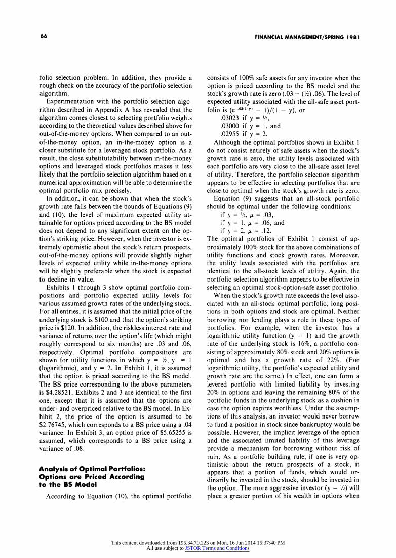
Exhibits 1 through 3 show optimal portfolio com- positions and portfolio expected utility levels for various assumed growth rates of the underlying stock. For all entries, it is assumed that the initial price of the underlying stock is $100 and that the option's striking price is $120. In addition, the riskless interest rate and variance of returns over the option's life (which might roughly correspond to six months) are .03 and .06, respectively. Optimal portfolio compositions are shown for utility functions in which y = 1/2, y = 1 (logarithmic), and y = 2. In Exhibit 1, it is assumed that the option is priced according to the BS model. The BS price corresponding to the above parameters is $4.28521. Exhibits 2 and 3 are identical to the first one, except that it is assumed that the options are under- and overpriced relative to the BS model. In Ex- hibit 2, the price of the option is assumed to be $2.76745, which corresponds to a BS price using a .04 variance. In Exhibit 3, an option price of $5.65255 is assumed, which corresponds to a BS price using a variance of .08.
Analysis of Optimal Portfolios: Options are Priced According to the BS Model
According to Equation (10), the optimal portfolio
consists of 100% safe assets for any investor when the option is priced according to the BS model and the stock's growth rate is zero (.03 - (/2) .06). The level of expected utility associated with the all-safe asset port- folio is (e .03(1-y) 1)/(1 - y), or
.03023 if y = /2,
.03000 if y= 1, and
.02955 if y = 2. Although the optimal portfolios shown in Exhibit 1
do not consist entirely of safe assets when the stock's growth rate is zero, the utility levels associated with each portfolio are very close to the all-safe asset level of utility. Therefore, the portfolio selection algorithm appears to be effective in selecting portfolios that are close to optimal when the stock's growth rate is zero.
Equation (9) suggests that an all-stock portfolio should be optimal under the following conditions:
if y = /2, M = .03, if y = 1, = .06, and if y= 2, , =.12.
The optimal portfolios of Exhibit 1 consist of ap- proximately 100% stock for the above combinations of utility functions and stock growth rates. Moreover, the utility levels associated with the portfolios are identical to the all-stock levels of utility. Again, the portfolio selection algorithm appears to be effective in selecting an optimal stock-option-safe asset portfolio.
When the stock's growth rate exceeds the level asso- ciated with an all-stock optimal portfolio, long posi- tions in both options and stock are optimal. Neither borrowing nor lending plays a role in these types of portfolios. For example, when the investor has a logarithmic utility function (y = 1) and the growth rate of the underlying stock is 16%, a portfolio con- sisting of approximately 80% stock and 20% options is optimal and has a growth rate of 22%. (For logarithmic utility, the portfolio's expected utility and growth rate are the same.) In effect, one can form a levered portfolio with limited liability by investing 20% in options and leaving the remaining 80% of the portfolio funds in the underlying stock as a cushion in case the option expires worthless. Under the assump- tions of this analysis, an investor would never borrow to fund a position in stock since bankruptcy would be possible. However, the implicit leverage of the option and the associated limited liability of this leverage provide a mechanism for borrowing without risk of ruin. As a portfolio building rule, if one is very op- timistic about the return prospects of a stock, it appears that a portion of funds, which would or- dinarily be invested in the stock, should be invested in the option. The more aggressive investor (y = /2) will place a greater portion of his wealth in options when
66
This content downloaded from 195.34.79.223 on Mon, 16 Jun 2014 15:37:40 PMAll use subject to JSTOR Terms and Conditions
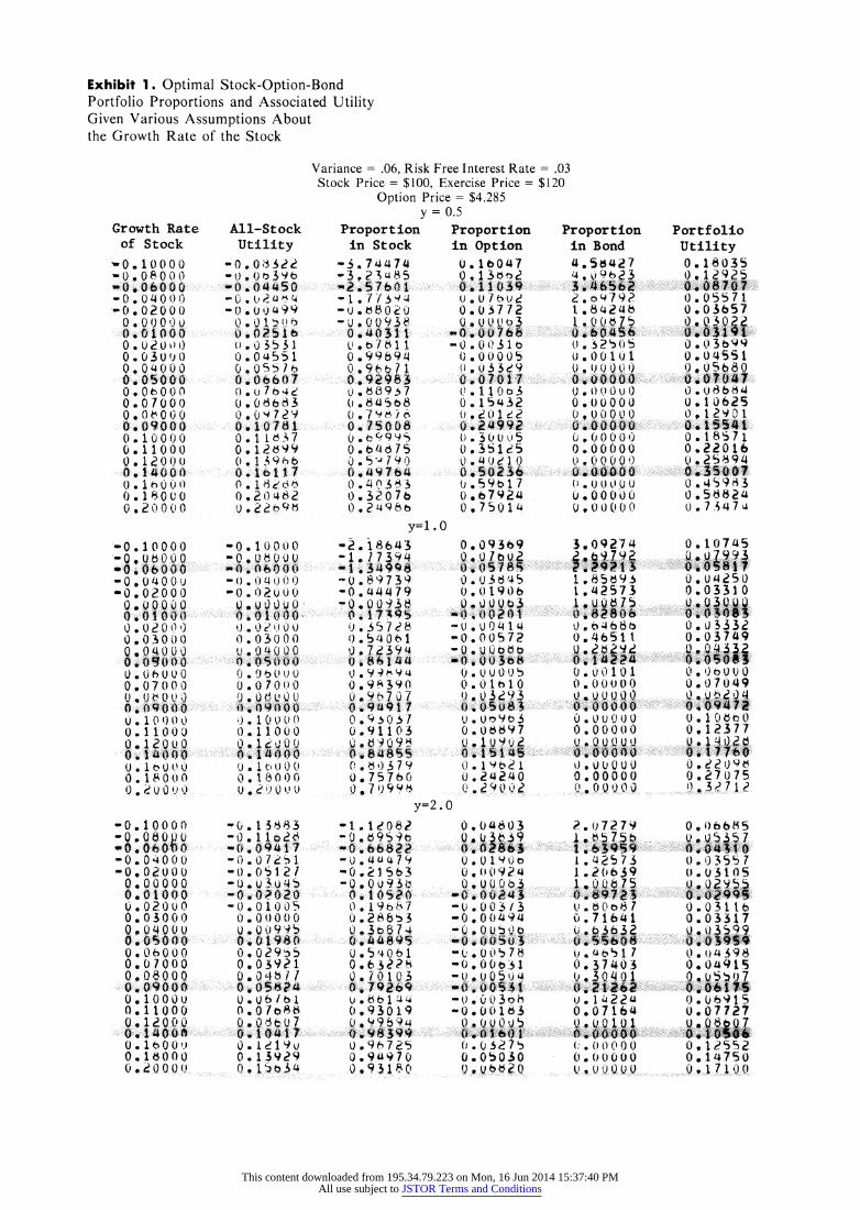
Exhibit 1. Optimal Stock-Option-Bond Portfolio Proportions and Associated Utility Given Various Assumptions About the Growth Rate of the Stock
Variance = .06, Risk Free Interest Rate = .03 Stock Price = $100, Exercise Price = $120
Growth Rate of Stock
0 , 08 0 0 -0. 00 0 0
-0,08000 0. 04000
-0 02000
0. OSO bO 0 * 000U 0.01000
0.0300 0
0, 04000 0.o7000oo
0 1 0 0 0 0
(. 1000" 0.. 1200)o
0.14000 0.1 0 0 0 0. 18000
-0.1o000
-0 .* 0400 0 'O.OqOOO
00:,0O 0 0. 01000
0 I 0 ? 0 0 ) 0 030 00
Q 1 0 0?0 0 0. 0 000
007 000
00 * 0 0 0
0 * 11 00 0 0
0 * 14000
-0.10000
0,1800000
o. I t0 ,o
0.10ooo0
; - .0000 0 . 0 0 0
-O.OqOO 0.07000
0. 09000 0.10000 0.1O000
0. 16009
0 . .80000
All-Stock Utility
-0.049392
-0., 045
.-)0 5 5
o Q 54 7 2 o.1 1 Id-l5;7b
0.04551 0,0.55
0 . u 76 b4 I0 * 0 663
0 10 7 2 9 0.1167 0.12699 0,1 396
o. 10. 1
-0 * 10000 - ,I . . o. U
-(). 0 000 -0. 02000
U 0.0U 0-
0. 0 c!' 0 0 0...030 0.0
0 0 19 b )
i 1 0 9 0 0 0. 017000
0.*101(00)
0 * 1 80 0 1
U.1 00 r 0
-0,11081
-0. 101 53 -0 * .01 00 5
0,0 0 9. 5
0.0 0921 00 '46 1b1
O.O/b! o0 01o08'i
o. 1197 0.1n399 0. 1^b'34
Option Price = $4.285 y = 0.5
Proportion Proportion in Stock in Option
- 3.74474 0. b047 - .7 ?015 0 .113 - 1. 7 / 9 t) u 0 7 b ud -ut ,80Q 0.03772 -U 00936 0oQ Uo3
b78 1 t -0.0031 0.99694 0.0005
(0.962$.3. 0.0703,1 0 ).8937 ( .110o3 (. 84Shb 0. 15432 0. 700 (.o 901 c?2
0 eb99U5 0. 30U .5 0.64075 0.351d5 0
? .4, 90 0 .5!020
0 40n3S o 59t17 0 3207b o.e67924 0 .498b 0, 75014
y=l.0 -2.18643
.1 .3A 446 -0. 89739 -0. 44479 -0 .0573a
0 .54061 0.7 7094
09 9 4 0 .9.390 o0 97 07
0 9 1 0 Q 71 0.91103
r, 3 e)79 0 75760
-1 1,d0891 -0 .9S9b
4- U 4 47 7' -0.21563 .-0:,0 u93.
0 196 7 1 0 2686eB53
0. 54 0 b 1
0. b b 11 4 0 93019 0. 9-95^4
0 96725 0.94970 0.93180
0O09369
0. 036,45 o,0 1906
-0.00572
0 .U 0 , 0: .
O.lh 1O
0t). ot3 C0.0 97
o,Y o e7 0.1514X 0 019d21
.02 4 , . 0 y=2.0
0.04603
0001900
U 00 3 3
-0Q * Qo090' -0 O (0. 0 9 S 4
0.00 :63 V r, o ( o f 7
- 0 ' 0, 3 o 0 -0.00163
. (....0..
0.05030 O.O030
Proportion in Bond 4. 5$427
20 o o79? 1.84246
. 007.5 u. 5 i U 0 1 0 0 1
(J0 '
0 0 0 0
0.00000 0.00000
0,000020
10 * (,0573
0o,00000
0. 00004)
0.00000 0 0 0 0 0
3.09274
1 .65 93 1.42573
0.46511
0.(010! 0 * 00 0 1
0 * U 0 00000 0.000 : 0
(J*()0.00000
?. 0 7279
I ,47573 I . 2 b 639 1...0 639
0 0 71 6 1 0.07600
0: 00300
Portfolio Utility 0,. 18035
0.03657
00 3022 0.04551 ,00560 0 I, S0 6b25
O.04bS4 0.10685 0,12901
0.18571 0.2206b O. 25694 0.45097 o .q% s 9 85 0.56824 U , 7 4 74
0.10745
0. 04250 0.03310
Q0. 0 3332 0.037t49
0, ')t 0 0 0. 7049
0 10 2 3 O 0.12377
. 7 1 0 7 !)..:....... .... .7...? .. ..
0.06650
0,03557 0.03105
.- 0 ... 0 ..395.
0.031 6 0.03317
0.03599
0. 04396
0 .077?7
0.!"1.552 0:* 14750 0. 1 7 1 )00
This content downloaded from 195.34.79.223 on Mon, 16 Jun 2014 15:37:40 PMAll use subject to JSTOR Terms and Conditions
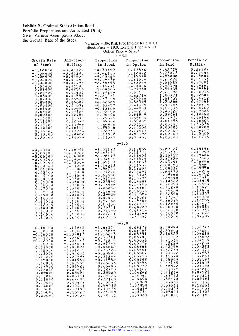
Exhibit 2. Optimal Stock-Option-Bond Portfolio Proportions and Associated Utility Given Various Assumptions About the Growth Rate of the Stock
Variance = .06, Risk Free Interest Rate = .03 Stock Price = $100, Exercise Price = $120
Option Price = $2.767 y = 0.5
Growth Rate of Stock
- U1 * o u 0 0
0 3 4 0 U
09 O 0 U 0
Q e
0 ,0100 O
O, * 11 0 ( 0 * 0 0 t
o0 0 ) 03 1. '0 0 0) )OO
All-Stock Utility
-0.0 <?3J ?o * 4o -4 * U}~qO0
^0.^M^ .1U ̂ )* (444
U ? 0 !4 bi 4 U.U 1, :iJ . * ( 5 '. .. 1 ). ^ V 45S 1
* 0 ? 5 ( 0.03't601
0* 8 e ) i
O * 1 tb 637 c) * 17 't 0. ld99
0 * 1i1 ' 1
.) * t ) 4 "q '
Proportion in Stock
-4 73) 5S9 -4
4 * '5 *
4 - 3. * '4 7
- i:1 s .431
- 1 , i ) , 1 31 *84 S
- 1)^ 7 2 . > ;
"0 * e1 9666
-t .. !,, 6' b d 8 ut * . U'h
. I (7 . 0 13 0 ) 1,Y<1 9
Proportion in Option
u <s;o * '4 'e
(). i118 U . 2 1 U U 4 (.3 * ?73n3
(.: I 5'14
3). 25 '1 4 4. *3 jb
* S 4, 99
l;'. b 5 13
0.59u65 U t>' 0i,
43 * i bU 1 0b~zl^Zi 0^ (? 4 5
Proportion in Bond
5.5775 . . ? 7. 7 .
3 * 6 S 7 9 ' 3 ;.!. / 2 * S 6 43
1 .. Ogi: u.I
. 4266
tl * 1 (6 '
3) * 691i 13
t). OOO u t
33 * ,V U t} t)
(4 U 3 ( o1
Portfolio Utility 0. , 1 85
0 . 960 u 1 U O*,7
-o .2a 7h?
0 * 5 7
U * i 3)9G6
0.1 7bo14*
1. uS54. 1 . 7"1 S
09 120)9 O, 11 / 1 4.11458
3U * 11 9 b U 0 i U 2 ;' 9 U.1 b
0, 1 480 7 3.1 . 4 9 b
U c' . I /
u) 5 i'u J 't
y=2.0 0063715 0. u 6 33 7' 2 0. 0581
. . 5 1 7 :',
O ? 'b 4C
3 3i / 1 3
090574' 0 . )5 CI 7 0. 059 1 2
(* (46 1 o 1
U.06771 09(4 '1 (969
-0.06000 - 40 I4 0 4 U
-0 0 2 0 0 0)
O, U 0 O, v 0. t* 0 4 13
0 * (44(0 33
0 0 0 ,.
0.07 000
0.10000
0 * t 400
0 . 2 . t) 3 J
- )10 1 0 0 -0 * 000
00 0 0 0o 0901000
() 3 0 000
O 9 * O 3) ) ) 0(0:0 :UO0
0 * 0000 0 0 O t0 0 * I 0 )00
(4 * 1 633.o .3 0 1 , l j (4 34)
0^ * J 0 '? 0
-{. * 103 O ')
- 0 0 0 - (' . () 3 ~i L: , -0 0 ? 0 (.;< 0
II * 0 0) <3 0
0050)00
,) * ,) 4 ,3 L 3( . I) * AO - 333
0., O 7 O u )(
0 \) 71 0 0 0 i, ^. 0 :000
0. 131 0)
tz, , p
"0 1 0 t 03v
1^ * 9 1
301 093 00
04. 1 1 0 i
- *0 1 O 1 9 .
-0. u 1 3 ,. 0 . (). 0 u 0
U. v l /'/
0 ?' 7) '
0. 1 . 1 w 1
(.1 . >o i
3. 011 97 - . 7j1 \ 1 -2?28177 1 *943 ?'1
-1 .551 7
- ) * b 12 3
- . , , ! I - ' * / ,J I
" '-0) ,' )
_ 04 .31e^$
- * 1 ") 1
0 >3) 2 7 $ 1
-1 .56374
-1.3 *4 (.)3 1
_ i0 '
5 i 3 t
)* t i. ? St'4
(.1 . 2 l<? . 0 , 4 ^ i 3n
. . 7 w 1
-, 0 S 3, | -9. V 0 5 ~
0.u ;~tc5 q'e,o
3,89127 3 553 9 1
<' 6 (' 5? 0 9 4.3491
~< 0 50 1 * ,7 70 1 49563
, 6 182
0 33 I I U 0.5.90
(0. () 0 000 0 00,0) 0
2. 4, 999 . 2 '.i,to 0 2, 10! 2 1 .9!03)2 1. /,b36
1 .$27S4 I ; 02 "2'4
1. s2.7e,22 1 , 1 b I/
0 * w / 1 ()
) *0 7 1s 4
0 561 7 i 1.5t51 l8 ( . 4 7 u d 9 0 .3:51 t 0( 1 b3a4 ^ 0.0548 1 U * I (.00 ( !3)
0 l1, 9t. 0 ?9119 9
O. 0 5O -5
0.0 6405 Q 0, 5 I
03 * 1 '1 1
o .1 o 5 U. 21 (4457
O .3 .' 6 7 t
0 , ( 7S94
0. 1 '7 9 '7
0 *,042 t 3
0. u( 3 7 -
0. ol 1846 0 0918'3
9 19 0.1 7301
tl' * 2) 1 6 (4
0) OT 11z 1 I
0t /? u I} 1 0
This content downloaded from 195.34.79.223 on Mon, 16 Jun 2014 15:37:40 PMAll use subject to JSTOR Terms and Conditions
Exhibit 3. Optimal Stock-Option-Bond Portfolio Proportions and Associated Utility Given Various Assumptions About the Growth Rate of the Stock
Variance = .06, Risk Free Interest Rate = .03 Stock Price = $100, Exercise Price = $120
Option Price = $5.653 y = 0.5
Growth Rate of Stock
-0.( 1O 0O -0 * 10 ) 0
-0 .04000 -C . 020U tc
V U) J0 0 0.) 0 0 o U O o. 01000
U QI f O ~) 0 ., 0 , 0) 0 o * 0 3 0 4 O
O * 0500)0
0 * 0 10Uo 0
0.09000 0 * 1 0 00O4h 0.110oo
O 1 4, (0t * .1 400(0 0 *
I A4 4t40
0 .2 00 U)i
)-0. () , i) 4 0 . 4 q 4i)4o
0O. u<'ou0
-0 0 u O u
0.01000
0 * 0 5'M4 0. 07 u O. o 10 :':
0. 0l90 O 0 (. ( 7 i) 0 0
0.09000
0 -I oo1)4 0.141 00 (. 1i0t0L0 0. I f)U ;)4 C. * ?4)OU
-0.1 0 0uo 0 -O 0 U 00 u
4) 00 .,0St 4( )
0 OUOuo 0 0 l l U
0o (o ( o 0 0
4 0
)U )
U . n)84 o)
0 .0,t00O 0 0 o 0 0 U
0.6700u
0 0 t 04 0.1 U I> 0 ,
0o 1 4 0 o)
0 *c tl) tJ
All-Stock Utility
-'). U?')5' -
.
0 4 4 5 O - t)()0 r <4 ̂ 4
-o L *
,)9 001 5 ie, t.0. tu 5 1 I
!i. '"r> b 7
4), 4 t; ol. a,o ) ! o o
C' * 11 'J 5 I
44. 1 89M
4) * I b 1 1 ;I e ts' ' 0.Ibll
t-0 I ,4) 0 l - . * 10 u U ii
- (, * ) 1..i ) }
U U (
.) 0 1) U 1 Q
i.OtJ090 0t. t4 f4)1?
O . 4) '.) O i
4. (5:4 u4 ) (4. * :t, Ui 4 44
);. O 0 i)00
!) . 1 I' (U !4 9 ( I11 t U i ' * 1 u t U, u4
4 1, u u 0 (; '
' C r' :. !, (0
4- 4 i 3'4 t 3
-0 1044112
l t 1 1 '
*- u(u 4 127
-0, 0(20O
-4) * (1 uiu 4). UOVw)e 0 , (019 /o
00!. ) : 7 o 1
I. . 1 U( 0.0i9ol
O ? '3 ,b o',,: ?
Proportion in Stock
-5.127e9 - ,. 1 .e.
_ y 1 u , - 1 7 1U
ll o
-,' * 9- 19 ' 4
- ')0 5 4 b 1
0.4) 74 . o
1O.b059.71 1 * u':' 1
1 .059191 1 U S * ' 4
0.b 1 / fu
s) * b9 I st
0.a771l U. 5. 3 7 u
Proportion in Option
0 17679 0. 1 ~ d 27 0.10036
44 * (441 / 3 - t). 1' ) 13
-) * 9 St 1
-!. u '1 .4 1
-0. 0599I V.)O^b^
-). o d 4 U 14t uu i5 t99 0.05510
0u . 1s / 19
U4 I 4 'n b
! . v M1 /1 v . 5eSCt6 U.1. b1 CJL
l.= . 0
- 1. 7u, e I ̂
-I .7al pi
-c, . 6 ( :8j 20
U. q 1 'b 0, 23 70 1 .os 5i 0; 1
.t'^1'i 1 uS~ ! 1j . b 99'
1 1 . 4 9 I 1 1 .Ob'~ 1 I .OUS03
01. 0(1 3
U, 0 19 L .s b
.1 . /e,7e. 4,, /?-e.4,,
y=2.0 -0)9. 921 2
-0o * 4'45 1s I
4) * 319 1 1 -(4. u n 1. S
09? '4 1 o
iJ 4 i :s4 1 0.51919
4 ) 0r 5 'Z' 7 1. 59o / t1 lJ . i991,
1 * , o l ! 4 09'vo9n5 r)9o/05bic
0) .0962
o(, 5 st10 a I; . ,:L t . 9
-0 4. ) obS -it,03528
4t) 09\881 -,. OS991
-u, (4b'-y 9 1
- . vu )'o l -0U J. 4)1 .
0 ? 1. t C < O ) t0 ^891
0 1 ' 14 -, 0Ib,('1sb,
. 0 1.54 3 U 0 .b!577
4 . 1i 52
ti0 * 1j ^00 -4 t -44 l
-'()0 , 04 i :. UO
* 05 lb
_-0. Of4'4
-4u, * L.4> 17 -4, . 4.') 5 fi
-04). O '5 1 -(). t .
-U . t(Ot 1. 4 )0. U 13u2?
4 ) 0 4 ),1 c. 5 f
Proportion in Bond
3. 950'9 .5 3.3'l 2.67508 1t.b c^Z 1.t02dO6 I *U. h
- 0 .0 0 00
-0. * 00000
-l . i (.w(.4) 44
.) 0 t 0 t)
. 0 0 () 0i 0. 00000 0 ), U 0 t) 0 t) . U 0 (0 0
0. uoo1o ;, . 0. I b06 (. ( 1 4(0,) 4O.00000
. (.' 9 3 0.0000
c . 9;$e) ,
L .441(i 0 t . a q t.},l 0 ) * 0 4) 5 8
4 . 04)404
4) U (4 4,4) t3
(400850
.4 * .155 ' '). i 1 fh ,
. , 0 C) U 5) 4444
u . O 5t t 0 0
- 0,00000
0 . 0 ( 0 0.U 3 . 0 U t J 0
0, 00 0i,
I .419014 1 . u. t. 'Y
?I } t^t} f '
. 49 1 v9
, * 0 090 1 u. 01 0 00
. Ot() 4) 7) 4
j (, ii,) U i4 04. 0'; 4 (: ) 1. )
(}, I } (i t'l J'.J J}
Portfolio Utility 0. 1953 0 o^77l
0. , 50 2 3
' * t'O 7 1
? e 8 7S 16. t 9 O 4
0 0 343 0.4 1 ( b . U 0.05/91
, 9 , 7 9 !, 4.0 I* 9 0 ?
7 )7
0, 04850 4.4 * is 253C 0 14377 (. t1 s o 0 .2043 u * ! 91b
40Ubb9
e. 04685
0.43000
0,4)3'95
0), ()79 9
4)0 i 0 i'5
0,0 , 7 44) 4 0 . O.) u 0 . 1t ,5 to
40. , 11.
U:, a q9)
(4. 1 7 7 4.) 0). ( 1 4 0
.
. 1 , 1 e ci i
.0 13575
0.03?9S1 ) 04)29 '. 5
*J . 0 38 1
) ij .4 43 1
41.01(7419 * 4.17'9
0I1 * !561
4* 1 2't 1
t(.13'412 4). 15"44 ',.
This content downloaded from 195.34.79.223 on Mon, 16 Jun 2014 15:37:40 PMAll use subject to JSTOR Terms and Conditions
FINANCIAL MANAGEMENT/SPRING 1981
compared with the logarithmic utility maximizer, while the more conservative investor (y = 2) will generally invest a greater portion of funds in stock.
When the stock's growth rate falls between 0% and the level associated with an all-stock optimal port- folio, optimal stock-option-safe asset portfolios con- sist of long positions in stock and safe assets with a
slight short (or writing) position in options. Note that when y = 1/2 and y = 1, the utility levels of these op- timal portfolios are not significantly different from those which might be obtained by either an outright stock or bond purchase. For example, consider the case of logarithmic utility. The largest discrepancy between the growth rate that can be obtained from an optimal stock-option-safe asset portfolio and the one that can be obtained by the more attractive of either an all-stock or all-bond portfolio occurs when the stock's growth rate is 3%. At this point, one could ob- tain a 3% growth rate with either stock or bonds, while an optimal stock-option-bond portfolio would grow at
only 3.749%. When the transaction costs of forming such a portfolio are considered along with the
analytical cost of determining the optimal portfolio mix, the increase in growth of .749% seems negligible.
When the growth rate of the stock is less than zero, optimal portfolios consist of long positions in options and bonds together with a short position in the stock. In such situations, the more aggressive investor will be
willing to short more stock. The mathematical for- mulation of this analysis assumes that the proceeds of the short sale can be reinvested, although this is not
always possible in practice. However, one can always sell stock from an existing portfolio and use the proceeds to invest in options and bonds. In this sense, the results have practical significance. Further, op- tions and bonds are purchased from the proceeds of the stock's short sale rather than options simply being written against a long position in the underlying stock. For example, if an investor expects the stock's growth rate to be minus 10%, and the investor is assumed to have a logarithmic utility function, an optimal stock-
option-safe asset portfolio will be expected to grow at a positive rate of 10.7%. Thus, one could improve the
expected growth rate of the portion of an existing portfolio which contains the underlying stock by 20.7% by simply selling the stock and purchasing op- tions and safe assets.
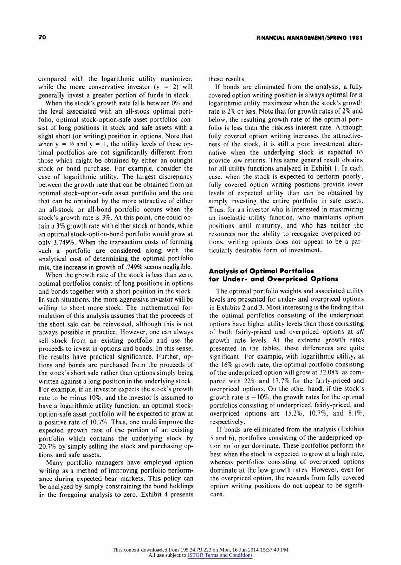
Many portfolio managers have employed option writing as a method of improving portfolio perform- ance during expected bear markets. This policy can be analyzed by simply constraining the bond holdings in the foregoing analysis to zero. Exhibit 4 presents
these results. If bonds are eliminated from the analysis, a fully
covered option writing position is always optimal for a
logarithmic utility maximizer when the stock's growth rate is 2% or less. Note that for growth rates of 2% and below, the resulting growth rate of the optimal port- folio is less than the riskless interest rate. Although fully covered option writing increases the attractive- ness of the stock, it is still a poor investment alter- native when the underlying stock is expected to
provide low returns. This same general result obtains for all utility functions analyzed in Exhibit 1. In each case, when the stock is expected to perform poorly, fully covered option writing positions provide lower levels of expected utility than can be obtained by simply investing the entire portfolio in safe assets. Thus, for an investor who is interested in maximizing an isoelastic utility function, who maintains option positions until maturity, and who has neither the resources nor the ability to recognize overpriced op- tions, writing options does not appear to be a par- ticularly desirable form of investment.
Analysis of Optimal Portfolios for Under- and Overpriced Options
The optimal portfolio weights and associated utility levels are presented for under- and overpriced options in Exhibits 2 and 3. Most interesting is the finding that the optimal portfolios consisting of the underpriced options have higher utility levels than those consisting of both fairly-priced and overpriced options at all
growth rate levels. At the extreme growth rates
presented in the tables, these differences are quite significant. For example, with logarithmic utility, at the 16% growth rate, the optimal portfolio consisting of the underpriced option will grow at 32.08% as com-
pared with 22% and 17.7% for the fairly-priced and
overpriced options. On the other hand, if the stock's
growth rate is - 10%, the growth rates for the optimal portfolios consisting of underpriced, fairly-priced, and
overpriced options are 15.2%, 10.7%, and 8.1%, respectively.
If bonds are eliminated from the analysis (Exhibits 5 and 6), portfolios consisting of the underpriced op- tion no longer dominate. These portfolios perform the best when the stock is expected to grow at a high rate, whereas portfolios consisting of overpriced options dominate at the low growth rates. However, even for the overpriced option, the rewards from fully covered
option writing positions do not appear to be signifi- cant.
70
This content downloaded from 195.34.79.223 on Mon, 16 Jun 2014 15:37:40 PMAll use subject to JSTOR Terms and Conditions
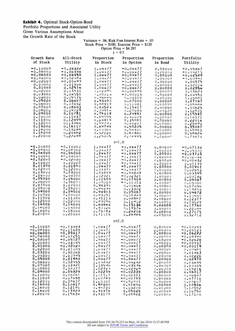
Exhibit 4. Optimal Stock-Option-Bond Portfolio Proportions and Associated Utility Given Various Assumptions About the Growth Rate of the Stock
Variance = .06, Risk Free Interest Rate = .03 Stock Price = $100, Exercise Price = $120
Option Price = $4.285 y = 0.5
Growth Rate of Stock
-0 . 1 0 0 0 0
-0. 06000 -0. )4OQ ilu
0 v 1)2)OO
O .2 u () O. ) 04 0 0.01000
.0 2 u o , 0u 0 0 0 0 090 ( 0 0 . h 1) 0 U
0. 09000 o.10uoo
0.1 40 000 O. 12000 olaooor
O.180o0(1 0 d 0
0 0 0 < 0! 0 ui U
All-Stock Proportion Utility in Stock
-)0 36S2
.* 04450
0.0 '4 49 4)0 0 1)40 0 *0251 0 14), il
4) *?) 7 b 0 06607
1), )9 1?9 0. 10781 0 1137 0. 18 99
e)1 4
* t 0.4 Z , 9e
4 .044 17 1.U 4 1 7 1 .4 4 4 /
1 *0U;4 77
I. ( 7 )7 / 1 * 444 / 7
I ? 41) i, j.,
44. /'9 1 '
} ?- 9 'I 9 $)
0. *,93 /
) * 459795
4) * ^4 t '4'
1) . c' 1 l *J , b () L 0
Proportion in Option
-0 044 77 - . 4 4 7 1 -0.0'4477 - I Ui)4 4 /
-1(*. )04417
-) u44 177 -:)i. s 3*75
O *0 1 I
4. 1. 41 , . 4 n0) e , U} . 5 u 0 d
0) * 0 S 105
* 61 b (C'I 41. ,4Od95
y=l .0
- ' . 4 4 77
-0 4477 -',Ji 4 4 / 7 -0. 44 7 -4)* J '4 7 / -0 0. 0 44 7
-' . ue J 1
,O i So * t). L) . ti o Ub )0 0 5 0 S 0.05067
i. 1. )q*92 u. t .) o l
y=2.0 - 0 0 44 1 7 -1 4 4 / I f1.4 4 7 41
- 0. 0447 . 44 74 / / " 1,4,~44.
-"0 * )44 7 / -0 *t 0 4'
-0 o4)1zS - )0 ,1 1" 1 -. 0 . i,) 1 2
00 , 1 ' 0 0 U) ?, V S / o 0.050d4 0. u e.6~'
Proportion in Bond
0. 00) 0 i0 t) * o (4I 0) (. J) 0.00000 ') . U 1 t) U t!
*0. 000 'I * 4)44014')
U.00000
. * V
0 0 04) o. 0 0
0.00000 0 . i) t0 0 0 '
) 0000)
0 * ooOUoo o ' (Io oU 4 O (. I) 1. 4 44
l'00000t,,i,
Portfolio Utility
. 005(7S u 0 1 0
-0. 02854 0 * 0 4 5 7
0 . 07047
* 1 /1 O? * 0v') 1b ,) ? 5. 4 0 * 35007
t . 447 1 0.i i35007
-0 .1 4)0000 -0. * 0 O 1) C) *,o rUoo 1* 00 i U 0 -0. 4 (J 0 0
O,0 U 0 U 0 0 * 0 0 0
00 * 0 7 01)1) 0. *o ( O 0.0700011 00 * O u 0
0.09000 o u o o )0" 0 .1 0700 0 * 09i000 0.11000
0. 14000 0 . o 001')(
0 010000 0 0. 80 '00
-O)*0600
-0. 02)00 0. 000)0) 0.01004 0. 020u )
0 0400)0 O. 0.000r
0.05000 00 6 0 u 0 0.07100
0)100') 00
0 t1 0 0 0
0 01200, 01()4000 0.(I)I V( ?
O.l~OO0 0. 16 00(0 0 * 2 0 1 *) 0
- 0. 10 0 0 0 "0.08 0'00
0. 06000 4* 1, ) 4 U )
0) 0 0 u0 0, 05)100)
.) /4 040
0 ?0/000 0 * 090)00 0) * lmn0o 0. 1 )1000)
0 * 14000 ') * l i,,) 00 ') . 1 j U 4.1 * 2 0 1 0 4)
-0.09417 -01. 7 / 51
-t) iQ) 4.
-) . 0127
- 0 4. 1)24
-0 .01 u08
0.01980 0.02955 0. 'O';'4 1
0c) 0,4,/1 '1 1). 0532a
'1. {)o 7r
0 . 1 04 11 0.12190 0)* 1 4929 04 1 I 9 4
I 0 .'4 14 7
1. 4 4 1 7
1.04477
I 4.0 4 1 1. dq, / 7
1. ) 4 4 7 /
1 991* S I * 01S 0 '4
0 * 1 1
) . 64664J
u 7 6/' 4 O. 1 ) I 5
1. .J1) 17 tI ) 4- 7 i
l. ; iq Ji 7
1. (la/477
1 * 0~44/ 7 4 *) 4 / 7
10.44//
1. (i;44/ 1 i 1. 4) 4 / / 1 .0441-
1i o a a ' 17
1. 4 4f5
1.,022i 5 t .'gq? 1o1
O.'931 !.
. O i)OOU 0 o . 0 o o 0. 00000 U. 0 00 )u 0t U. 0 )U 0 4 4) 0 0000(
O. 0 0 000
J) o 0 4') 0-. c(:, 000 4) * 4u) )o 4 0 0 u 0 0 0 Uo 0 U u 0. 0000 9.0 0 U !)0.J
) U )IJ0 0 ') 4) , 00 O)0 41
1) * 00000
0. 000)00 u. (9oo )
U. 0 oU U
4 ) 0 uo 0. 00000 U
0 0) ) )
0, 0 0 0 t 0. ) 0 0 (J
1. OO41 I') ,i.) 00 0U4 0
0. t) ? u 0 .0 U i) 0 i
,.0 U 01 ) 0
4 * (01 0 0 (0
0.000110, 4)! * 4)041', 4) ,.
-) *0 71 - .0 i) li)j
_e ,) iJ (: y)e4
o - U 5 ) 4 4)
'0 7. 0l3 -U . t) () ( . )
.0* 07
0. ui ?. $i )
0. 13795
0.0 7 v )
u. 09478
'. I 4). 1. .4 ) 0.17760
(. 1L 47 5 .214)1l
- 00 * 12 4 "0. Ob 22
-0. (4 0
.0 9771U
* 00119e,
(it I 74 1 .4 1
11 4b3
0) . (129 70 4i) . o99
0 * 4 4 75
u) 7 7 1 u *1 , 5 4? 1
40.) 0506
*i * 1 4475(1 '" . I / 14 )
This content downloaded from 195.34.79.223 on Mon, 16 Jun 2014 15:37:40 PMAll use subject to JSTOR Terms and Conditions

Exhibit 5. Optimal Stock-Option-Bond Portfolio Proportions and Associated Utility Given Various Assumptions About the Growth Rate of the Stock
Variance = .06, Risk Free Interest Rate = .03 Stock Price = $100, Exercise Price = $120
Option Price = $2.767 y = 0.5
Growth Rate of Stock
-0.1(!0000 - 0 * 00 0 0
-0, 04)00 0
0 U 0 U 0 I
U. 02(J 0 0 03000 0 .0 4 0 () ' 0 04000
0 .05000 0 06700 0
0 b 1 2O ) 0.1 0 000')
0. OUo)O
0.11000 0 I 0 o01)
0.14000
0 . o 0 U)
-0. 20 U) -0 16000
0 .01000
0. )4000u 0.0 000
0. 1T)OU
0U )* 1 0 0: 0 . 0 0 0.10000 0.07 0t 00 0 ?0000 0. 09000 . 10 to O)
0 I .0 0 0 0? 10001
0 1 h (3) 0 0 i 8 0 0 0 ?. 0U <(
-0 1000
0 060 0 0O. OOOOl -0.0400')
- 0 0 0 0 01 0,000 0U 000000
0J. V ''O )i U
9) * I 0 0 i 1)
0 0 7 t 0 0
0 o60f'.U
O) . t? 7l u) u ) n * 7 00o0 (0 . O90!0
0.110') u 0. 1(00 U
0 ?14000
0 1 * 0 0:))
All-Stock Proportion Utility in Stock
-0.04322
0) 5 1 o 0
0. 455 1
0 * Q / S ~ 1 0 , 0O 1
0 . 5') 7 or3 ) * 0i/r'4.2'
,* 0 1) 2 S
1, * 1S 9 190 -0. 1811 7
- *
9,)
0 ?U 000
01000
o'1 * ijQ 9 8)
I * 0 00
0 ? 0 3 ') 00 0 Q* ? 4 '. ) ') 01.05000
. '07000
. 10 1 0 0
.o * o o ' ' ) I 0 l) 0
)*018;00') (0 * 0 0 l Ci 0
-0,l1 .o.. -0.) 094 17
-0). t51o8 - ,). 0 03 '?
-0 J 02020 -,3.,)1 j;)
0. * 01980
0( * 1' / *t 1 00 7 u
0 ^' lo 7 0) 0 4 1 /4
00 1 2 ? 9: ) (1l
*
>5
1 * 'Uor2*4 1 * . 2 ? : h 1.0~844
(I . 9 : 8 1 F: 0.95812
0. 0517 1 0< * 1 /c ' o.d1702 0. 7 b5b4 0/ U I 43 0. o.O1t'
0,5 t 4 1
0 -4 1 .
i4
.1 5 0 4 7
0.q95132
1. 931)784)
0.92324
0;,wl 9o 4
"1 .c 1 4 0
i * /5370
9l.*2~ t1 /
7)^ 7 0 S
1. 0264 1 ? :) 2? ,'4 15
1 . 0 2 '4 8 1i ?01 / 7 c',
1.0U1 7 ^ 1 . 1 <? i, l.7r 1 t!
0. * '4.. 904 0. 9/! ! 4
<.) . '^. < 4G ?> t) * 9 4 4 .4 0.944/. 4 0 . 5 t w)
* s i': ; 4
Proportion in Option
-0 * ueO46
-0 U02646
O. ,} q?4 1 4 1; *10 * u 0t
U I u5e t
0.) 4 b51 ,9 .2244$o U. d c o (' 0,31399
114. , C8 % 9
* 45 1 7 9 (10.50179
! * 54 n '4
* 7 0540
, . 35 1 v=l. 0
-0) .0264 -0) j 8 4 b
1001968
' . o , 1 ~ 4 (). - '/ 4
U.1 .902 0, 1 5 1 0
).1A2 /b
'.1 e2
-0,. 04bh 0* 2646 - 9j ., d '4 6 - :; ,) ,- 8 - - 0 / 2t, -'.1 '*' 1O7
,1 * '1,,1 5 '")
- 0 . 02 o 0
0.0 4 / 4 * ( I 41 49)
*.:.055 7 uu * '> 91 i 0. , 4 5 '). ,:)99
Proportion in Bond
',. 0 00 u 0 ".0 U 0 00
',. OOOu 0. 00000 3 . \) 0 Ut '.) 0.0 u u o o 0 * 0 0 U 0 U
0 . 0 000
* 0 0 u O 0 (I 0 0 00000 (I. t) i 00 ) '" 0 0 U U 0i 'U , ") 0: U 0 0i)
0 .00000
. 00 09 U U ~J 0 U 0 0 ) . 0 0 t U
U}. 0 0 t) 0 t0 0* 1 0 U)
0 00000
k). t 0 t) tI)
' * OUUO U U * 000 0 0
u. OOU0
:) 0)0 0 i 0
0U. 00000
i) 0?0 L0 ' 'i o . 0 0 0 0 Ui
! U 0 0' 0 U o u u) , u, u
. 000(0 O. 10 (1 O(
0 0 0000 ;. * (! 1 1) 911!
. 0 ) t O 0.) 1) ? '.9 U U 9
0. 00)0 0
. * 011' 0 U ,
0. OuOOU
' J 000 00
it 0 (: U U t
') . 00000
j* ) O;t)1 i) *) * 0 u u u 1
Portfolio Utility
V-0. O1 8 . * o57 49
U *) e ( U; 6
0.04750 ^ 04 710
U) * 91 4 u ! 7 0 * 1 e6d t 0 .16.39
.3 ds49:
U4 * 4tS 15 0 * 54330
0 .8 709
t .d,71S5 1 ( 1 . 1$ - 0 b 17 7
-0. 0527 7b
-t) .! 931 0 * u 00 l
i,. 03590
. 00505 O* (* 0 1 '4 5
I. i 3684 .i 4 i .
0 .2521 i aa4 7 ; 3, ; 7 I. t,
u,.qt?W9
-U * 1169
-0, 07906 -* 1 0 4
0. (40 55
-.01o77
V( * 9 1 S33
0.01983 ., * ,i , i2 r 3 0u 3 9 S 4 ,, * S 0
00U b 0 6 0 v / 1 37
i'),ub 5 , 2 0.11998
.1 * I a
' ,J L ii i
This content downloaded from 195.34.79.223 on Mon, 16 Jun 2014 15:37:40 PMAll use subject to JSTOR Terms and Conditions
Exhibit 6. Optimal Stock-Option-Bond Portfolio Proportions and Associated Utility Given Various Assumptions About the Growth Rate of the Stock
Variance = .06, Risk Free Interest Rate = .03 Stock Price = $100, Exercise Price = $120
Option Price = $5.653 y = 0.5
Growth Rate of Stock
-0 100 00
*0.o 0o6000 -0 . 0 64 0 0 -0. i02000
0 . 0 uU( ) .01000994 0.01000
0.0 , o
0 0 0.03000
0 0 t O L) 0 0 0 7 0 0 0. 0 700
O.l 1 000
0. 1 4000
0 1 o0 0 0 b 000 0O624OO0
-0.1* 0000 -0. 00000 -0. 0000
09 0 4) o4) 4
0.001000
0607000 O.0 1 6 0 0 u. )0000 0. lf.t Ou0
0. 1100 0 * 12) 0 0 0. i 40i0 0. 1 4000
0. 1600)0 0. 20000
-. 1 00) 0
-0. 0OoO -004. 0 00
.1 * 20 I)) 0.0000
0o0300t) 0,u4000 4 05000
0.01000
0 )6 03000
0.05000
O * 0 4)4) 0 0I 0 0 0. oO0- o
061100') 01ZuOG
1 2bIO
0. 1 7 00
t). ! OOO
All-Stock Utility
-0.063cd? -0. * 4) :5o9 -004450
0 *.' 1) oos,,1io
()O. 0 4, 1b
o . o) 7 '4 ? o * 0891 3
o0 10781
i) . t I b T
) 1.3 0 8
* 1) 0 00 -). O4U! 0 i
-0.06000
00 0 0 00 0.010400
o ),) )O 4) U
0.0300U
0.0)500 0 0 0 ) vu 00 o o U 0. t) P ) 0 O
) * 1 0 i)
0. 140040 0U. 1 20(1
u, 4 0) 4) 0
-(). 1 3'83.
.04 09417 -, ,. 1 7, i 1 -0. , O I 2 -u.4 03o45 -0* ?0?0)
0. O 99 0. 01980
, 0 039 '
0 . 1 c) 0 * '0 4 oV* I 1)3 '0~. 1'rd
Proportion Proportion in Stock in Option
I .05199 1 * O 4 3 ' 1 1 .,)$991 10. )5991
1 .05991 1.4) O991
1 o*il9l
1. 6 % 9 4 1 1.05991 1 6 tzt 99
1 . )02 ,)
0.94503 ()* i /'S
96 7-4}'2 0.6917? 0,5I<279
i04t7724
1 6 (,5iJ91 1 6991
1(.05991 1.0S9O1 I 05991 1.05991
1. Ob91 1 .5Vl91 1. o0S991 1 *9 4" ' 9 1 1. V)"9q1
I . .0o 3 9 ; 1 1.U13091 1 - it 1 - 1 7 0.9932$
a . 19306
06. .) b b 1
1. *'i ' 991 1I 05991 I.0 '~91 16059W1
1 iB t:,99j 1 *,)'~9 ! 1 05 !9 1
1. )5991
1 .05991 I. ,')59W1
1. ) 59 1
1*) b 77 ,' t ? ?4959 1,4 149
1. o o 1 0.98707
-O.OSv'I
- 4) r cJ 5 9 5 I
-00),59Sl -0. 05991
-0O5991I -0 059 1 -0.05991
4 4) 1 5 4
-0.0599i
) .0549
,y=l . . 0
-O.05914l
-) . 0991 -06. 3J 91
0t. 0599 1 . 0 5991
. . U0699
-9 * 4 4 99
-0.0009
-0,. 0bs6 0.114/4
-0.05991 -6. 05 91
0.4)05991 6.). 9S9 1
0 .) 6 ^ 9
^0 IS' IS -0. () 5991
o *4 4 94
0 2 14/3
-O, 1 0599
-0. 05991
0.u0:91
0.4. 4311
Proportion in Bond
0. 00000 4) .0904.1)
0. O 0 O
o. 0000
4 ) u (4 0 0) J. 0 0 0 0 0 . 0 00000 J 0 t)! 0 ()
0 00000 .). 4) 0 i0) 9 0 * 00000
0 * (0000
0. 00000 (4.004)90
1). i)UOO I)
4) 4)4)) 0 U'
J,0 0 00)
1*1) 4' ) 94
* ) 9 tj 4) 4) 4 * 9) 4) 44),
9 69 0 9 9 4 i.! OOOu . l)
4) 6 4) 4j )4)4)
9 ,
4(t)4) ii
0 * 0 00
0) 00000
0. 00000 0 00 t 0o0
0 000( 0 .)U ) U0 0.00000 4)64) k 000 0 .0o00
. 0 0 o) 0t/
1l O, u 0 'J * 0 0 ) 0 ('
Portfolio Utility
-0.0 4465
. O 4o
007?4 i 0.04318
U. o8730 Li) 9 7 4 3
* 1 J 534 0.1U377
o. 1 15? . 37986
4 * 4)5b-7S
6.9, 1,)595
-0. t)64 - 0 0 . 4 6 4 4/ -0) *8 9 144 7
. UU 1 0 t 7 oud5 /44 . 0 3339 0 . 94 () 91 O .U4832
0. (4 4 I 0 0, 4 a 3t :
4- 04 1 5
0,0 hS 3
0. 1465! , 1 7 / 4 5 1.2 1 4i1)9
*. 6 'b 9 1
-0 06521 -O0) 65/9 *07 * h4)- 87 0
-0. lh ? 9
010471 6
I i. ~ '9 I.
.1 * '1-y 94
0 69 ' : 1 3:
. 0 t1 9/ 9. 15" d
This content downloaded from 195.34.79.223 on Mon, 16 Jun 2014 15:37:40 PMAll use subject to JSTOR Terms and Conditions
FINANCIAL MANAGEMENT/SPRING 1981
Portfolio Sensitivity to Interest Rate and Variance Changes
In Exhibits 1 through 6 the riskless interest rate and variance of stock returns are held constant at .03 and .06, respectively. Assuming that the option is priced according to the BS model, an increase in the riskless interest rate will result in an upward shift in the stock growth rates for which all-safe asset and all-stock portfolios are optimal. [This is evident from Equa- tions (9) and (10).] Moreover, it can be shown that, for any stock growth rate, the optimal proportion of port- folio funds allocated to safe assets will never be less than the optimal proportions associated with a lower interest rate.
On the other hand, if the variance of stock returns is increased, the growth rate associated with an all-safe asset optimal portfolio will fall while the growth rate associated with an all-stock portfolio will rise (assum- ing that options are priced according to the BS model using the increased variance). Since option prices will increase as the variance increases, the optimal per- centage of portfolio funds invested in options will decrease with an increase in the variance.
Conclusions
This paper describes an algorithm for determining the optimal composition of portfolios consisting of a single call option, its underlying stock, and a safe asset, assuming that the investor desires to maximize an isoelastic utility function. Optimal solutions are analyzed given various assumptions about the return and risk characteristics of the underlying stock and the prices of options relative to the Black-Scholes model.
In general, optimal solutions consist of long positions in options and stock when the stock price is expected to appreciate significantly. When the price of the stock is expected to decline, the optimal solution consists of a short position in the stock with the proceeds of the short sale being used to purchase call options and safe assets. A strategy of writing options only provides significant improvement over an all- stock or all-safe asset portfolio when the option is overpriced relative to its equilibrium value.
Future research in this area might explore the effects of the investor's holding period on optimal portfolio compositions. In addition, the diversifica- tion provided by options on more than one underlying stock might be considered. Although optimal port- folio weights would differ from those found in this
study if the analysis were extended into these areas, it is unlikely that the general implications of the present analysis would be altered.
References
1. F. Black and M. Scholes, "The Pricing of Options and Corporate Liabilities," Journal of Political Economy (May/June 1973), pp. 637-654.
2. F. Black and M. Scholes, "The Valuation of Option Contracts and a Test of Market Efficiency," Journal of Finance (May 1972), pp. 399-417.
3. D. P. Chiras and S. Manaster, "The Information Con- tent of Option Prices and a Test of Market Efficiency," Journal of Financial Economics (June/September 1978), pp. 213-234.
4. J. C. Cox, S. A. Ross, and M. Rubinstein, "Option Pricing: A Simplified Approach," Journal of Financial Economics (September 1979), pp. 229-263.
5. E. Elton and M. Gruber, Finance as a Dynamic Process, Englewood Cliffs, N.J., Prentice-Hall, 1975.
6. D. Galai, "Empirical Tests of Boundary Conditions for CBOE Options," Journal of Financial Economics (June/September 1978), pp. 187-212.
7. D. Galai, "Tests of Market Efficiency of the Chicago Board Options Exchange," Journal of Business (March 1977), pp. 167-197.
8. J. Gould and D. Galai, "Transaction Costs and the Relationship Between Put and Call Prices," Journal of Financial Economics (June 1974), pp. 105-129.
9. R. E. Johnson and F. L. Kiokemeister, Calculus with Analytic Geometry, Boston, Allyn and Bacon, Inc., 4th ed., 1969.
10. R. Klemkosky and B. Resnick, "Put-Call Parity and Market Efficiency," Journal of Finance (December 1979), pp. 1141-1155.
11. H. A. Latane and R. J. Rendleman, Jr., "Standard Deviations of Stock Price Ratios Implied in Option Prices," Journal of Finance (May 1976), pp. 369-381.
12. R. C. Merton, "Theory of Rational Option Pricing," Bell Journal of Economics and Management Science
(Spring 1973), pp. 141-183. 13. R. C. Merton, M. S. Scholes, and M. L. Gladstein,
"The Returns and Risk of Alternative Call Option Port- folio Investment Strategies," The Journal of Business (April 1978), pp. 183-242.
14. R. Schmalensee and R. Trippi, "Common Stock Volatility Expectations Implied by Option Premia," Journal of Finance (March 1978), pp. 129-148.
15. C. Smith, "Option Pricing: A Review," Journal of Financial Economics (March 1976), pp. 3-51.
16. R. Trippi, "A Test of Option Market Efficiency Using a Random Walk Model," Journal of Economics and Business (Winter 1977), pp. 93-98.
74
This content downloaded from 195.34.79.223 on Mon, 16 Jun 2014 15:37:40 PMAll use subject to JSTOR Terms and Conditions
RENDLEMAN/OPTION INVESTMENT STRATEGIES
Appendix A. Description of the Mathematics of the Portfolio Selection Algorithm
Simpson's Rule, which is found in most calculus texts, is used to derive a close approximation for the evaluation of all the integrals in Equations (7), (8a), and (8b). According to Simpson's Rule, if f(z) is a con- tinuous function over an interval (a, b), if n is an even integer, and if (z0, z, . . ., Zn) is the regular partition of (a, b) into subintervals, then:*
b f(2)d2
b- a(f(zo) + 4f(z,) + 2f(z2) + 4f(z3)...
+ 2f(Zn-2) + 4f(zn-) + f(Zn)). (A-l)
In Equation (A-l), the term (b - a)/n is the length of the estimation interval. f(zi) is the value of the func- tion to be integrated at the point Zi, where Zo = a, z1 = a + (1) (b - a)/n, z2 = a + (2) (b - a)/n, and so on. The accuracy of the approximation depends upon the number of points at which the function is evaluated with the maximum error being (b - a)5 K/(180n4), where K is chosen such that K > | f"' (zi) | for every zi in the interval (a, b).
A binary search is employed to find optimal port- folio weights. The values of qs and qw are iterated within their feasible regions until the values of both Equations (8a) and (8b) are within the bounds ? .0005. In some instances, it is impossible to achieve this degree of accuracy and the search is stopped at the last feasible solution which is evaluated. When there appear to be corner solutions due to the implicit con- straints on qs and qw which are described earlier, the objective function is restated as a function of q,, and the derivative of the restated objective function is evaluated with respect to q,.
In both problems, boundary terms for +oo and -oo are chosen so that all standardized logarithmic returns from the stock above (or below) these values can be ig- nored without changing the nature of the assumed log- normal distribution to any great extent. The upper boundary which is employed is MAX(B + 5, 5), and the value of the lower boundary term is MIN(B - 5,5).' At a minimum, these bounds include 99.99994% of the outcomes of the probability distribution and therefore appear to be reasonable. Each interval is divided into forty subintervals between its upper and lower bounds.
Appendix B. Optimal Portfolio Composition with Continuous Revisions
Here it is shown that the optimal continuously reallocated portfolio consists entirely of stock when the option is priced according to the BS model provided that ts = r + (y - /2)U2 and entirely of bonds when t = r - V/2a (the subscript, s, is added to denote variables which refer to the underlying stock). To facilitate the analysis, recall that, at the BS price, the option is a perfect substitute for a continuously reallocated stock-bond portfolio. Therefore, options can be omitted from the analysis.
Given continuous portfolio revisions and a port- folio policy that calls for constant portfolio weights, the return of the optimal stock-bond portfolio will follow a lognormal distribution with a growth rate of #p, variance of op, and expected instantaneous return of E(Rp) = Ap + l/2rp per unit of time.
Let q8 represent the proportion of the portfolio held in stock and (1 - q8) the proportion held in bonds. The investor's portfolio selection problem is to choose the value of q1 that maximizes E(HI-Y)/(l - y).
With constant portfolio weights, the value of the portfolio will follow a lognormal distribution, and the investor's utility function can be stated as
E(U(F)) E(H1-) 1-y
=EXP(,p (1 - y) + 1/2a ( -y)) (B-1 ) (1 - y)
Assuming a constant proportion, qs, of portfolio funds are held in the stock and (1 - q,) in a safe asset, the portfolio's instantaneous expected return becomes
E(Rp) = q,E(R,) + (1 - q,)r = q9,( + I/2a72) + (1 - q,)r.
By recognizing that the portfolio's variance is
a2 = q 2, q, 0,, (B-3)
and the portfolio's growth rate is
Up = E(Rp) - 1/22,
*This description of Simpson's Rule is adapted from Johnson and Kiokemeister (9, pp. 271-275). Equation (B- 1) can be restated as follows:
(B-4)
75
(B-2)
This content downloaded from 195.34.79.223 on Mon, 16 Jun 2014 15:37:40 PMAll use subject to JSTOR Terms and Conditions
FINANCIAL MANAGEMENT/SPRING 1981
E(U(H)) = EXP(qsE(R) (1 - y) - /2aq2(1- y) +
(1 - q,)r(1 - y) + /2qa (1 - y)2) (B5) (1- y)
The value of q8 that maximizes E(U(H)) is obtained by taking the derivative of E(U(H)) with respect to q., setting it to zero, and solving for q,. The optimal value so obtained is
E(Rs) - r qs= y2
As + l/2 - r (-6) (B-6) yEqha
Equation (B-6) implies that qs = 1 when I9 = r + (y - 1/2)af and qs = 0 when As = r - S/2j.
FINANCIAL MA NA GEMENT ASSOCIA TION ELEVENTH ANNUAL MEETING
The Financial Management Association brings together practicing financial managers from industry, financial institutions, and non-profit and governmental organizations, and members of the academic community with interests in financial and investment decision-making. The eleventh annual program, October 22-24, 1981, at the Stouffer-Cincinnati Towers in Cincinnati, Ohio, will stress the interrelationships between theory and practice in financial and investment management.
1981 Annual Meetings
Dates: October 22-24. 1981
Place: Stouffer-Cincinnati Towers Cincinnati, Ohio
Program Participation:
Meeting Arrangements:
Placement Information:
H. Robert Bartell, Jr. PMI Mortgage Insurance Company 601 Montgomery Street San Francisco, California 94111 (415) 788-7878
Professor Waldemar M. Goulet College of Business Administration Wright State University Dayton, Ohio 45431 (513) 873-3175
Professors Verlyn D. Richards and Randolph A. Pohlman
Department of Finance, Calvin Hall Kansas State University Manhattan, Kansas 66506 (913) 532-6892 and 532-6868
76
This content downloaded from 195.34.79.223 on Mon, 16 Jun 2014 15:37:40 PMAll use subject to JSTOR Terms and Conditions