Optimal location of intermodal freight hubs

Illia Racunica

Institut Eurecom

2229 Route des Cr�etes, B.P. 193

06904 Sophia Antipolis, France

and

Laura Wynter

PRISM, Universit�e de Versailles

and INRIA

Domaine de Voluceau, B.P. 105

78153 Le Chesnay, France

Abstract

Attempts at reducing the externalities of freight transport in Europe

are generally focused on the incorporation of a more signi�cant use of rail

into freight itineraries. One new scenario for increasing the share of rail

in intermodal transport involves the development of a dedicated subnet-work of freight rail lines. Within this European Union project, the use ofhub-and-spoke type networks, in combination with �xed-length shuttle ser-

vices for freight, are under discussion. We present this innovative projectand the proposed optimization model. The problem is cast as a nonlinearconcave-cost hub location problem. A linearization procedure along with

two e�cient variable-reduction heuristics are proposed for its resolution,making use of recent results on polyhedral properties of this class of prob-

lems. Computational experience is provided on the European network of

potential hub terminals.

The most recent scenarios under study for integrating freight transportation in

Europe e�ciently and with minimum social and environmental cost involve exten-

sive use of intermodal transport. The intent of these new transport scenarios is to

1

make maximum use of rail transport, not only for long haul and low value freight

distribution, as has been the case, but over medium-length distances as well.

To permit rail to be competitive with road haulers in Europe, one of the few

policies that remains viable is the use of a subnetwork of dedicated or semi-dedicated

(that is, in which freight is given priority) freight rail lines. Indeed, it has been

observed that complete integration with passenger rail services has rendered it di�cult

to increase the market share of rail in the freight transport sector, since freight slots

are generally given only at night, or between passenger trains during the day. In all

cases, on mixed-use lines, passenger services are given priority, to the detriment of

the quality of service o�ered by rail freight providers.

The primary reasons cited for the predominance of road haulers are the low travel

times they o�er, and their high exibility in terms of departure times. Currently, in

Europe, freight rail schedules are planned weeks in advance, and last-minute requests

can be accommodated only through insertions between passenger trains and planned

freight service. Consequently, exibility is severely limited. The development and

integration, therefore, of a dedicated or semi-dedicated freight subnetwork is the focus

of several large-scale European Union research projects (see INRETS �nal reports:

EUFRANET, IQ, and SCENES [7]). With respect to reducing freight travel times

on rail services, high-speed freight rail services are being considered as a potential

component of the proposed freight subnetwork.

Within this context, investigations have examined the use of network con�gura-

tions prevalent in airline transportation, such as shuttle services operating on regular,

frequent schedules. Of particular interest is the fact that shuttle services would per-

mit the use of a viable hub-and-spoke network con�guration for rail freight transport,

in that rapid and reliable hub-to-hub transfers could be included in freight itineraries.

These itineraries could then include high-speed freight train services on a few corri-

dors. Fixed-length shuttle services mean reduced terminal times, since trains need

not be recon�gured, and would allow far greater exibility, since reservations would

not be required, much as is the case with airline shuttles.

An essential feature of shuttle services, and hub-and-spoke networks in general,

is the economies of scale that can be gained by consolidation as well as by reducing

shunting costs. This is crucial for rail freight transport, since current operating costs

are high compared to those of road haulers, and freight consolidation would permit

substantial cost savings to the rail operators.

This paper is concerned with devising a model for the conception of such an inno-

vative hub-and-spoke network for multimodal freight transport on dedicated freight

2

rail lines. Of particular interest is the incorporation of the scale economies resulting

from freight consolidation at hub terminals. Desired results of the model include in-

formation on the optimal hub locations: How much freight can each (potential) hub

capture? What percentage of the market can the shuttle services take from both the

current direct complete block train service, and from the share of the road haulers?

Which corridors can become competitive enough to warrant the construction costs

associated with high-speed freight train services? How would an evolution of freight

ows e�ect these conclusions?

Since it is necessary to evaluate both the market share of the hubs themselves and

of the lines (shuttle services versus direct train service and road service), coupled with

the need to explicitly include economies of scale, the choice of a model representing

each path explicitly appears judicious as opposed to a more compact arc-based formu-

lation of the network ow problem. Furthermore, the importance of the construction

and development costs in converting terminals into \mega hub" nodes, capable of

handling shuttle services, leads us to adopt a network design approach.

We therefore model this rail freight network design problem as an uncapacitated

hub location problem with concave increasing costs on certain links. The concave

costs represent economies of scale that can be obtained between two hub nodes, and

from hubs to non-hub destination terminals. Explicit capacity constraints were not

included, as one desired result of the model is to evaluate the maximum average

frequency attainable by rail on any freight corridor.

The objective of the model is then to minimize a linear combination of hub con-

struction costs and travel costs, where the latter takes into account the e�ect of freight

consolidation where applicable. The rate of increase of direct (origin-to-destination)

complete block train service is taken to be a linear function of distance, since the

number of wagons is directly proportional to the tonnage carried. Conversely, given

the �xed composition of shuttle services, the marginal cost to the user on these lines

decreases considerably with increasing ow, as the additional cost for each ton hauled

is lower than the cost of running the train. Similarly, for non-shuttle services between

hub terminals and destination terminals, su�cient consolidation is believed to allow

for some economies of scale, though less than can be attained on the �xed-length

shuttle lines.

The resulting model, described in the following section, is cast as a nonlinear

mixed-integer program. Constraints on the model concern the maximum number of

hubs that can be opened, as well as the maximum number of hubs traversed in any

path. The latter constraint is included implicitly within the de�nition of the ow

variables. We present further some recently developed polyhedral properties of this

3

model. In order to correctly model the in uence of train frequency on choice decisions

and on travel costs, we have chosen to implicitly include frequency e�ects through a

calibration of the cost function, rather than through the use of a dynamic model with

time as a parameter. This model is therefore similar to that of frequency network

design with frequencies as derived output, within the context of the classi�cation

proposed by Crainic (2000).

In Section 2, we discuss solution procedures for the model. To solve the program

e�ciently, a linearization scheme is used for the nonlinear ow term. The linearized

problem is then coupled with a very e�cient heuristic that permits approximating

the e�ect of the concave costs with a linear optimization solver. We demonstrate as

well the e�ect of incorporating the polyhedral information into the formulation.

Section 3 provides numerical results on the European rail freight network and

interprets the bene�ts acquired through the use of this model. Finally, in Section 4,

we discuss a number of interesting avenues to be explored within the scope of this

problem.

1 Formulation as a nonlinear mixed-integer hub

location model

The problem of the optimal location of hubs in a network has received attention over

the past decade due to its importance in air transportation, and also in telecommuni-

cations. See, for example, Bryan and O'Kelly (1999), Campbell (1994), or Campbell

(1996). The objective is to determine a posteriori the number of hubs to be opened

and the paths used in the network, where a hub is opened only if it is pro�table

to do so. The de�nition of \pro�table" is given in terms of hub opening costs and

travel time savings, where the latter are, in principle, due both to su�cient consol-

idation and as well as trip time reduction. The basic model, presented below, has

been studied and some algorithms proposed in the references O'Kelly et al. (1995),

Klincewicz (1996), Skorin-Kapov et al. (1996), Ernst and Krishnamoorthy (1998),

and Hamacher et al. (2000).

1.1 The basic hub location model

Let us de�ne �rst the graph G = (N ;A) where N is the set of all terminal nodes,

and the set of potential hub nodes is H � N . The set of arcs is de�ned as A, where

4

each arc is weighted by its travel time. Paths in the graph are identi�ed as a sequence

of the nodes traversed, where this number is limited to at most two hub nodes per

path by the de�nition of the path variables. The standard uncapacitated hub location

model is then given as follows:

minx;z

F (x; z) :=X

i2N

X

j2H

X

k2H

X

l2N

cijklxijkl +X

j2N

fjzj (1)

subject to

X

j2H

X

k2H

xijkl = dil; 8(i; l) 2 W; (2)

X

j2N

xijkl � Qilzk; 8k 2 H; (i; l) 2 W; (3)

X

k2N

xijkl � Qilzj; 8j 2 H; (i; l) 2 W; (4)

xijkl � 0; 8j 2 H; 8k 2 H; (i; l) 2 W; (5)

0 � zj � 1; 8j 2 N ; (6)

zj 2 f0; 1g; 8j 2 N ; (7)

where d 2 <jWj

+ is the vector of demands over the set W � N 2 of origin-destination

(o-d) pairs. The ow variables are given by x 2 <jN j2�jHj2

+ , and z 2 f0; 1gjHj is the

vector of discrete decision variables indicating whether a hub is to be opened or not.

The constant Qil is de�ned such that Qil � dil; (i; l) 2 W, in which case, equa-

tions 3 and 4 ensure that hub i (resp. j) is open for the ow through that hub to be

non-zero. Costs on the path (i; j; k; l) are given by cijkl, while fj is the cost associated

with converting the terminal j into a hub node.

1.2 Taking into account economies of scale

In order to take into account the cost reductions that are obtained by consolidation

at hub nodes, the technique used in the standard hub location model is to apply a

so-called discount factor on the interhub links of the network, so that the per-unit

price on interhub links is lower than that on extremal links of the network. See, for

example, Ernst and Krishnamoorthy (1998), Hamacher et al (2000), O'Kelly et al.

(1995), or Skorin-Kapov et al. (1996) where the authors use the following objective

function, which makes use of the discount factor, �, where 0 < � < 1:

5

cijkl := cij + �cjk + ckl: (8)

That is, the unit cost per distance is lower between pairs of hubs than otherwise, but

the marginal costs on all links are constant with ow.

It is clear, however, that objective function (1) with costs given by (8) does not

model scale economies, which require that the the marginal price decreases with

increasing ow, in which case, the cost function must be strictly concave increasing,

rather than linear. Clearly, this simpli�cation is costly in terms of accuracy of the

solution since large and small ow values all receive the same discount.

To deal with this de�ciency, we generalize the de�nition of some of the terms

in (8). While it is technically feasible to generalize the de�nition of all three terms

in (8), our motivation is to accurately model the econmies of scale arising from the use

of hub-and-spoke shuttle service for freight transport. Therefore, direct (origin-to-

destination) complete block train service is taken to be a linear function of distance,

since the number of wagons is directly proportional to the tonnage carried. Shut-

tle services between two (mega-) hub nodes are designed to operate with a �xed

composition, so as to reduce shunting costs; consequently, the marginal costs de-

crease considerably with increasing ow on hub-to-hub shuttle lines. Similarly, for

non-shuttle services between mega-hub terminals and destination terminals, su�cient

consolidation, along with somewhat reduced shunting costs at the mega-hub node is

believed to allow for some economies of scale, though less than can be attained be-

tween two mega-hubs. To summarize, then, we have included nonlinear concave cost

terms between pairs of mega-hub terminals, and from mega-hub to destination ter-

minals, where the nonlinear coe�cient on the latter routes will be higher than on the

former.

Furthermore, since a primary objective of the model is to evaluate the market share

of the hubs with respect to currently existing direct, complete block train itineraries,

it is necessary to include paths not passing through the hub nodes as well. Flow on

a direct path from i to l is therefore represented by the variable xiill, where nodes i

and l are not hub nodes. Note that itineraries passing through exactly one hub are

implicitly de�ned in the original model, where the ow is given as xijkl with j = k.

Adding these characteristics to objective function (1), we obtain:

(x) :=X

i2N

X

j2H

cij

X

k2H

X

l2N

xijkl +X

j2H

X

k2H

c

1jk(x) +

X

k2H

X

l2N

c

2kl(x); (9)

where c1(x) and c2(x) are nonlinear discount functions. Then, the objective function

6

can be expressed as:

minx;x;z

F (x; x; z) := (x) +X

(i;l)2WnH

cilxiill +X

j2H

fjzj (10)

Note that the constraint (2) must be replaced by:

X

j2H

X

k2H

xijkl + xiill = dil; 8(i; l) 2 W (11)

so as to include ows on direct routes.

We �rst make the following assumption.

Assumption 1 The functions c1jk

: <jWj

+ 7! <+ (resp. c2kl

: <jN j�jHj

+ 7! <+) are

continuous, concave increasing functions for all nonnegative x, for all pairs of nodes(j; k) 2 H2 (resp. (k; l) 2 H �N ).

Then, we have the following property of the objective function.

Proposition 1 The objective function F (x; x; z) is a continuous, nonnegative, and

concave function of (�; �; z), a�ne in (x; x; �), for all nonnegative x; x.

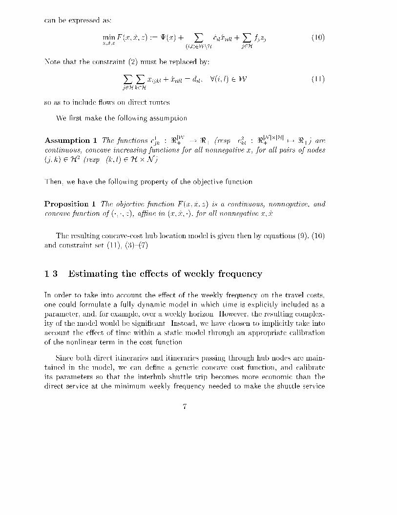
The resulting concave-cost hub location model is given then by equations (9), (10)

and constraint set (11), (3){(7).

1.3 Estimating the e�ects of weekly frequency

In order to take into account the e�ect of the weekly frequency on the travel costs,

one could formulate a fully dynamic model in which time is explicitly included as a

parameter, and, for example, over a weekly horizon. However, the resulting complex-

ity of the model would be signi�cant. Instead, we have chosen to implicitly take into

account the e�ect of time within a static model through an appropriate calibration

of the nonlinear term in the cost function.

Since both direct itineraries and itineraries passing through hub nodes are main-

tained in the model, we can de�ne a generic concave cost function, and calibrate

its parameters so that the interhub shuttle trip becomes more economic than the

direct service at the minimum weekly frequency needed to make the shuttle service

7

origin, imega-hub, k

destination, l

mega-hub, j

Direct route

Origin-to-mega-hub

Shuttle service (between mega-hubs)

Mega-hub-to-destination

Figure 1: Direct versus hub-based itineraries for a typical origin-destination pair

a

c(x)

direct link cost function

inter-hub or hub-to-destination cost function

x

Figure 2: Cost function calibration between a direct and hub-based trip leg

viable. Consider the Figure 1 which represents the itinerary choices for a given origin-

destination pair, (i; l). The Figure 2 illustrates the calibration of the concave cost

curves with respect to the linear, direct (complete block train) cost curves on a typical

example. The two curves should intersect precisely where the shuttle services becomes

advantageous. Quantitative data on this point of intersection permits calibration of

the cost function parameters.

Letting the concave interhub discount function c1jkbe given by c1

jk= a

1jk(P

(i;l)2W xijkl)0:5,

we set

a

1jk(X

(i;l)2W

�xijkl)0:5 = �cjk

X

(i;l)2W

�xijkl (12)

8

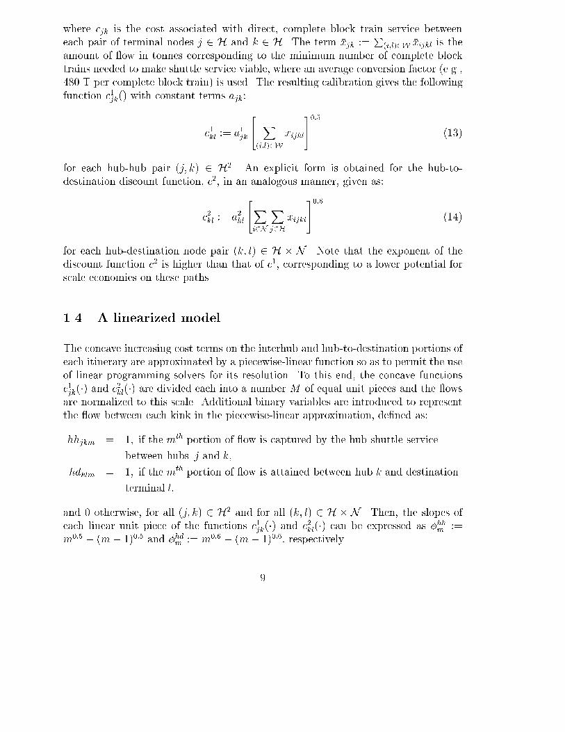
where �cjk is the cost associated with direct, complete block train service between

each pair of terminal nodes j 2 H and k 2 H. The term �xjk :=P

(i;l)2W �xijkl is the

amount of ow in tonnes corresponding to the minimum number of complete block

trains needed to make shuttle service viable, where an average conversion factor (e.g.,

480 T per complete block train) is used. The resulting calibration gives the following

function c1jk() with constant terms ajk:

c

1kl:= a

1jk

24 X

(i;l)2W

xijkl

350:5

(13)

for each hub-hub pair (j; k) 2 H2. An explicit form is obtained for the hub-to-

destination discount function, c2, in an analogous manner, given as:

c

2kl:= a

2kl

24X

i2N

X

j2H

xijkl

350:6

(14)

for each hub-destination node pair (k; l) 2 H � N . Note that the exponent of the

discount function c2 is higher than that of c1, corresponding to a lower potential for

scale economies on these paths.

1.4 A linearized model

The concave increasing cost terms on the interhub and hub-to-destination portions of

each itinerary are approximated by a piecewise-linear function so as to permit the use

of linear programming solvers for its resolution. To this end, the concave functions

c1jk(�) and c

2kl(�) are divided each into a number M of equal unit pieces and the ows

are normalized to this scale. Additional binary variables are introduced to represent

the ow between each kink in the piecewise-linear approximation, de�ned as:

hhjkm = 1; if the mth portion of ow is captured by the hub shuttle service

between hubs j and k;

hdklm = 1; if the mth portion of ow is attained between hub k and destination

terminal l;

and 0 otherwise, for all (j; k) 2 H2 and for all (k; l) 2 H � N . Then, the slopes of

each linear unit piece of the functions c1jk(�) and c

2kl(�) can be expressed as �hh

m:=

m0:5 � (m� 1)0:5 and �

hd

m:= m

0:6 � (m� 1)0:6, respectively.

9

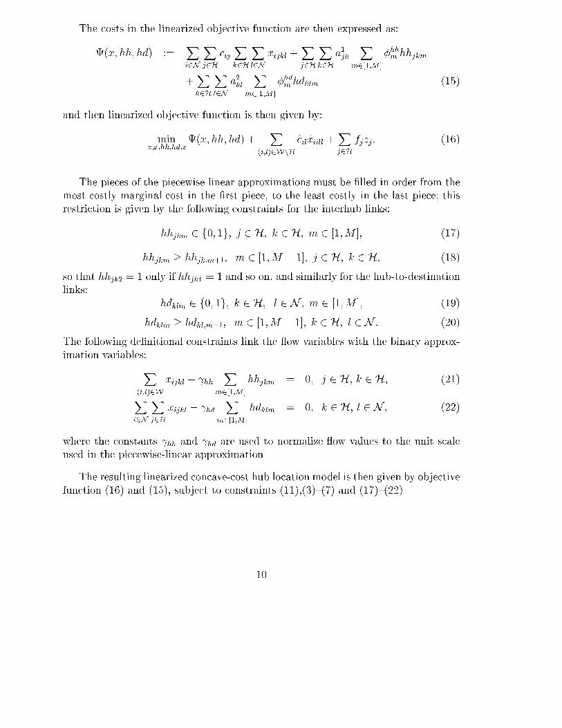
The costs in the linearized objective function are then expressed as:

(x; hh; hd) :=X

i2N

X

j2H

cij

X

k2H

X

l2N

xijkl +X

j2H

X

k2H

a

1jk

X

m2[1;M ]

�

hh

mhhjkm

+X

k2H

X

l2N

a

2kl

X

m2[1;M ]

�

hd

mhdklm (15)

and then linearized objective function is then given by:

minx;x;hh:hd;z

(x; hh; hd) +X

(i;l)2WnH

cilxiill +X

j2H

fjzj: (16)

The pieces of the piecewise linear approximations must be �lled in order from the

most costly marginal cost in the �rst piece, to the least costly in the last piece; this

restriction is given by the following constraints for the interhub links:

hhjkm 2 f0; 1g; j 2 H; k 2 H; m 2 [1;M ]; (17)

hhjkm � hhjk;m+1; m 2 [1;M � 1]; j 2 H; k 2 H; (18)

so that hhjk2 = 1 only if hhjk1 = 1 and so on, and similarly for the hub-to-destination

links:

hdklm 2 f0; 1g; k 2 H; l 2 N ; m 2 [1;M ]; (19)

hdklm � hdkl;m+1; m 2 [1;M � 1]; k 2 H; l 2 N : (20)

The following de�nitional constraints link the ow variables with the binary approx-

imation variables:

X

(i;l)2W

xijkl � hh

X

m2[1;M ]

hhjkm = 0; j 2 H; k 2 H; (21)

X

i2N

X

j2H

xijkl � hd

X

m2[1;M ]

hdklm = 0; k 2 H; l 2 N ; (22)

where the constants hh and hd are used to normalize ow values to the unit scale

used in the piecewise-linear approximation.

The resulting linearized concave-cost hub location model is then given by objective

function (16) and (15), subject to constraints (11),(3){(7) and (17){(22).

10

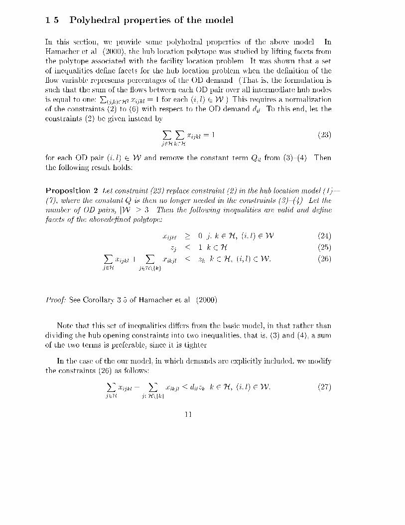
1.5 Polyhedral properties of the model

In this section, we provide some polyhedral properties of the above model. In

Hamacher et al. (2000), the hub location polytope was studied by lifting facets from

the polytope associated with the facility location problem. It was shown that a set

of inequalities de�ne facets for the hub location problem when the de�nition of the

ow variable represents percentages of the OD demand. (That is, the formulation is

such that the sum of the ows between each OD pair over all intermediate hub nodes

is equal to one:P

(j;k)2H2 xijkl = 1 for each (i; l) 2 W.) This requires a normalization

of the constraints (2) to (6) with respect to the OD demand dil. To this end, let the

constraints (2) be given instead by

X

j2H

X

k2H

xijkl = 1 (23)

for each OD pair (i; l) 2 W and remove the constant term Qil from (3){(4). Then

the following result holds:

Proposition 2 Let constraint (23) replace constraint (2) in the hub location model (1){

(7), where the constant Q is then no longer needed in the constraints (3){(4). Let thenumber of OD pairs, jWj � 3. Then the following inequalities are valid and de�ne

facets of the abovede�ned polytope:

xijkl � 0 j; k 2 H; (i; l) 2 W (24)

zj � 1 k 2 H (25)X

j2H

xijkl +X

j2Hnfkg

xikjl � zk k 2 H; (i; l) 2 W: (26)

Proof: See Corollary 3.5 of Hamacher et al. (2000).

Note that this set of inequalities di�ers from the basic model, in that rather than

dividing the hub opening constraints into two inequalities, that is, (3) and (4), a sum

of the two terms is preferable, since it is tighter.

In the case of the our model, in which demands are explicitly included, we modify

the constraints (26) as follows:

X

j2H

xijkl +X

j2Hnfkg

xikjl � dilzk k 2 H; (i; l) 2 W: (27)

11

Next, we show that (27) is both valid and facet-de�ning for the model (1), (11),

(3){(7).

Proposition 3 The inequality (27) is valid and is a facet for (1), (11), (3){(7).

Proof: The �rst part of the proposition is straightforward, since the sum of the OD

ow can never exceed the sum of the OD ow through the hub k and the OD ow

sent on a direct route. The second follows as a direct extension of Proposition (2)

above.

2 Solution method

In O'Kelly and Bryan (1998), the authors present a hub location model with piecewise-

linear costs, and test the model on a 20-node network using application-speci�c linear

programming software. Each piecewise-linear approximation to their concave cost

function, however, has only three pieces. This a�ects, in particular, the threshold of

e�ciency of the interhub trip as compared to (in our case) the direct trip. In addition,

�xed costs for hub opening are not included in the above reference.

In our case, the model makes use of from 25 to 100 linear pieces to approximate the

nonlinear cost functions for each hub-to-hub and hub-to-destination pair, meaning in

practice that the linear approximation is very close to the original nonlinear function.

Although we can eliminate some of the possible hub-hub and hub-destination pairs

by simple pre-processing techniques, the number of binary variables is on the order

of 10,000. To solve the resulting model, we therefore develop an e�cient heuristic

method to solve the linearized problem.

In the case of linear hub location models, a classic resolution method consists in

performing a Benders decomposition and solving independently the 0-1 programming

problem over the binary variables z, which indicate whether or not a hub is to be

opened, and the linear network ow problem for a �xed set z of open hubs. However,

the �rst phase integer programming master problem is generally very di�cult to solve

if there is no particular structure to exploit.

Rather than decompose the problem in this fashion, we have chosen to make use of

recent polyhedral properties of the linear hub location problem and solve the problem

as a large mixed-integer program. Indeed, preliminary results have shown the cuts to

12

be quite e�cient at removing non-integer solutions of the hub-location variables, zi.

For more information on this work, the reader is referred to [6] (or to a related work

on the single allocation problem by Sohn and Park (2000) for the case in which the

number of hub nodes is exactly three).

However, as opposed to the abovementioned references, our problem in the ow

variables is still a very di�cult problem to solve. This is due, of course, to the

piecewise linear relaxation of the concave cost curves. Indeed, the number of binary

variables associated with the segments of the piecewise linear curve is on the order

of several thousands. In order to approximate exactly the concave cost curve, it

is necessary to impose the constraint that the second piece of each piecewise-linear

function is used (that is, hhjk2 = 1) only if the �rst piece is used (that is, hhjk1 = 1),

and similarly for the third piece (hhjk3 = 1 only if hhjk2 = 1) and so on for all

remaining pieces, and each of these variables (hh and hd) is binary.

To solve the model in practice, then, we have devised a variable-reduction heuristic

which solves a sequence of relaxed subproblems, in which constraints (17) and (19)

are replaced by

hhjkm 2 [0; 1]; j 2 H; k 2 H; m 2 [1;M ]; (28)

and

hdklm 2 [0; 1]; k 2 H; l 2 N ; m 2 [1;M ]: (29)

The following variable-reduction heuristic technique successively reduces the number

of free variables, thereby forcing the initial pieces to 1, allowing only the �nal used

piece to be fractional, as should be the case.

2.1 A variable-reduction heuristic: heuristic 1

1. Set Mjk := M and Mkl := M for each (j; k) 2 H2 and each (k; l) 2 H �N .

2. Solve the (relaxed) subproblem with constraints (28) and (29) replacing (17)

and (19).

3. For each arc (j; k) 2 H2 with fractional values of hhjkm,

(a) Calculate the total amount of ow assigned to the arc. That is, obtain

yjk :=X

m2[1;Mjk ]

fhhjkm j hhjkm > �g

for 0 < �� 1.

13

c(x)

piecewise-linear cost curve

concave cost curve

1 2 3 4 M=5x = 2.5

hh-m is 0.5 for each piece m, in 1,...M

flow on this pair,

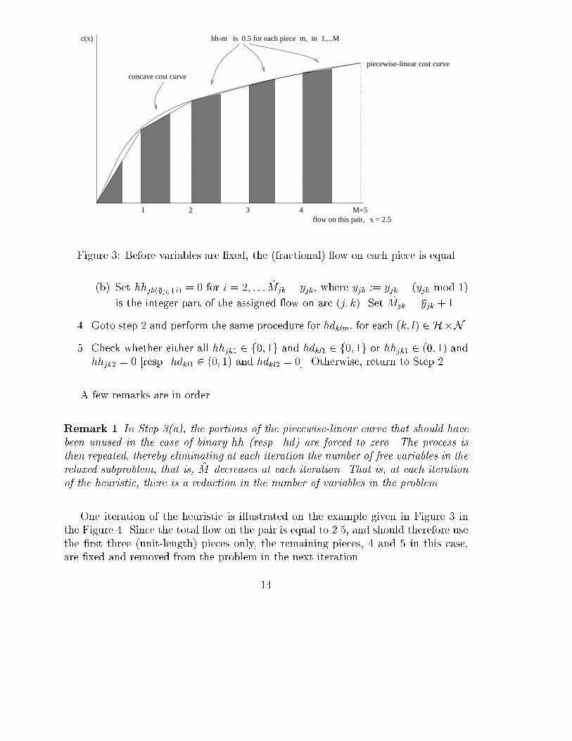
Figure 3: Before variables are �xed, the (fractional) ow on each piece is equal

(b) Set hhjk(�yjk+i) = 0 for i = 2; : : : Mjk � �yjk, where �yjk := yjk � (yjk mod 1)

is the integer part of the assigned ow on arc (j; k). Set Mjk = �yjk + 1.

4. Goto step 2 and perform the same procedure for hdklm, for each (k; l) 2 H�N .

5. Check whether either all hhjk1 2 f0; 1g and hdkl1 2 f0; 1g or hhjk1 2 (0; 1) and

hhjk2 = 0 [resp. hdkl1 2 (0; 1) and hdkl2 = 0]. Otherwise, return to Step 2.

A few remarks are in order.

Remark 1 In Step 3(a), the portions of the piecewise-linear curve that should have

been unused in the case of binary hh (resp. hd) are forced to zero. The process is

then repeated, thereby eliminating at each iteration the number of free variables in the

relaxed subproblem, that is, M decreases at each iteration. That is, at each iterationof the heuristic, there is a reduction in the number of variables in the problem.

One iteration of the heuristic is illustrated on the example given in Figure 3 in

the Figure 4. Since the total ow on the pair is equal to 2.5, and should therefore use

the �rst three (unit-length) pieces only, the remaining pieces, 4 and 5 in this case,

are �xed and removed from the problem in the next iteration.

14

c(x)

piecewise-linear cost curve

1 2 3 4 M=5x = 2.5flow on this pair,M^=3

Flow on pieces 4 and 5 are fixed to zero

Active variables in the next iteration

Figure 4: Illustration of heuristic 1 on the example of Figure 3

Remark 2 Note that, in the �rst iteration, if any hhjkm > � and fractional, thenall pieces satisfy precisely hhjk1 = hhjk2 = : : : = hh

jkMdue to the constraints (18)

and (20). (See Figure 3 for an illustration.) Therefore, setting the last piece to zerohas the e�ect of \forcing" the higher (marginal) cost pieces to be used, or shifting the

ow to a di�erent path. This characteristic holds for the remaining iterations, with

the index M reduced at each iteration for which there are fractional ows.

Remark 3 As a stopping criterion, it is thus su�cient to check the value of pieces

m = 1 and m = 2 only, since either each piece i 2 Mt (where M

t is the number of

free variables remaining at iteration t) has an equal fractional value, or else only thelast piece is fractional.

For example, if one considers Figure 3 to represent the output of the relaxed sub-

problem resolution at some iteration, then Step 3 of the variable-reduction heuristic

would add the following constraints (letting the decision variable for each piece be

expressed as hhm): hhm = 0 for m 2 [4; 5], since the total ow on the path is 2.5,

and the piecewise curve is de�ned by 5 pieces. In other words, variables hh4 and hh5

are removed from the problem in subsequent iterations.

15

2.2 A faster variable-reduction heuristic: heuristic 2

The following heuristic speeds up the variable reduction process of Step 3 in heuristic

1. In particular, in Step 3(c), the additional fractional pieces are �xed to at most

the value of the fractional part of the total ow present on the route. (In Figure 3,

then, the piece m = 3 would have the following constraint added to those de�ned by

heuristic 1: hh3 � 0:5.)

1. Set Mjk := M and Mkl := M for each (j; k) 2 H2 and each (k; l) 2 H �N .

2. Solve the (relaxed) subproblem with constraints (28) and (29) replacing (17)

and (19).

3. For each arc (j; k) 2 H2 with fractional values of hhjkm,

(a) Calculate the total amount of ow assigned to the arc. That is, obtain

yjk :=X

m2[1;M ]

fhhjkm j hhjkm > �g

for 0 < �� 1.

(b) Set hhjk(�yjk+i) = 0 for i = 2; : : : Mjk � �yjk, where �yjk := yjk � (yjk mod 1)

is the integer part of the assigned ow on arc (j; k). Set Mjk = �yjk + 1.

(c) Set hhjk(�yjk+1) � yjk mod 1.

4. Goto step 2 and perform the same procedure for hdklm, for each (k; l) 2 H�N .

5. Check whether either all hhjk1 2 f0; 1g and hdkl1 2 f0; 1g or hhjk1 2 (0; 1) and

hhjk2 = 0 [resp. hdkl1 2 (0; 1) and hdkl2 = 0]. Otherwise, return to Step 2.

Heuristic 2 should therefore converge faster, since the problem is more constrained

at each iteration, the price to pay being naturally that the local solution obtained

may be of inferior quality.

3 Computational experience and analysis

The numerical experiments of the hub location model were carried out on the data set

described in the Appendix. The set of terminals used was obtained from the Euro-

pean Freight Railway Network (EUFRANET) study [7] by selecting the 32 terminals

16

# hubs, # nodes, # pieces Heuristic 1 Heuristic 2 Exact solution

3-4-25 8277 (0.3%) 9744 (18.1%) 8252

3-5-25 25,273 (3.9%) 28,223 (16.1%) 24,315

3-6-25 37,899 (4.9%) 39,610 (9.6%) 36,138

4-5-15 23,352 (4.8%) 26,024 (16.8%) 22,274

4-6-15 38,130 42,337 {

5-6-15 36,249 39,649 {

Table 1: Validation of the Variable-reduction heuristics

in the Alpine region with the largest international intermodal freight ows. Potential

mega-hub nodes were those with the highest gravity potential to attract freight con-

solidation. Flows between all terminals were obtained from the NEAC data set for

combined transport tra�c.

First, however, the two variable-reduction heuristics are validated on a subset of

the data.

3.1 Validation of the variable-reduction heuristics

In this section, the two variable-reduction heuristics are tested on a subset of the data

small enough to permit an exact resolution of the linearized subproblem by branch

and bound. The Table 1 provides the results of these tests. The �rst column of

the table provides the characteristics of the data set, in terms of number of possible

hub nodes, total number of nodes (where each pair of nodes has a non-zero demand

to every other pair), and the number of segments used in the approximation of the

concave cost curve. The integer programming solver of CPLEX (version 6) was used

to obtain the exact solution. Similarly, the CPLEX linear programming solver was

used to solve the linear subproblems in the two heuristics.

Note that, for test sets of more than three hub nodes, the integer programming

solver was unable to provide a solution, even with the number of segments reduced

to 15 for each concave cost curve. As concerns the quality of the two heuristics,

the �rst heuristic is clearly superior to the second, more constrained heuristic. The

�rst heuristic provides solutions within �ve percent of the optimal value, for those

test sets for which an optimal value was obtained. On the other hand, the second,

more constrained heuristic provided, on average, solutions on the order of 15% more

costly than the optimal solution. Since the computation time of the both heuristics

is very reasonable (less than 0.5 seconds for each of the test sets above), the �rst

17

Costs, fj fi : zi = 1g fi : zi = 0g �I := fi : zi 2 (0; 1)g, �(z�I)

random 1 0,1,3,4,5,6,7,8,9,10,11,13 { j�Ij =2, � = 0:04

random 2 0,1,3,11,13 5,6 7, � = 0:05

high est. 0 12 12, � = 0:16

med. est. 0,6,11 13 10, � = 0:08

low est. 0, 5, 6, 11 10, 13 8, � = 0:07

Table 2: Results on the full-size data set

heuristic is clearly preferable. It is this heuristic that was therefore used in the code

for solving the overall hub location problem. Numerical results onthe overall problem

are presented below.

3.2 Numerical results on the full data set

The purpose of the model developed is to permit studying the potential of a hub-

and-spoke type network of intermodal freight terminals in Europe. One key corridor

for freight transport improvement in Western Europe is the Alpine crossing. The

numerical results presented in this section are taken from the application of the model

to this important corridor.

The number of nodes in the graph is 32, representing the major sources of emis-

sion and reception of intermodal freight tra�c in Europe. Of these, 14 terminals

were selected as potential mega-hub nodes; that is nodes which are candidates for

construction of e�cient container swapping equipment and �xed-composition freight

shuttle service. All tests in this section were therefore run on this full set of 32 nodes,

14 potential hub nodes, and 100 linear pieces for each of the concave cost curves.

The CPLEX linear programming solver was used to solve the overall problem

along with variable-reduction heuristic 1. The addition of the constraint (27) was

su�cient in eliminating non-integer solutions on very small data sets, on the order of

those presented in Table 1.

To test the model and solution method on the full-size data set, initially, two sets

of random hub opening costs were generated. The results are provided in Table 2.

The �rst column provides the type of hub-opening costs used in the test set. The

second column gives the number of hubs with values zi identically 1, and then those

with values equal to 0. The last column provides the number of hubs with fractional

values of zi and the average fractional value. The main thing to observe is that, when

18

fractional values were present in the results, the values were very small, particularly in

the tests with randomly generated hub opening costs. In the last three tests, realistic

hub-opening costs were used (with high, medium, and low estimates of the costs).

The quality of the polyhedral information good, but could be stronger. This is seen

from the fact that the average value of the non-integer results is signi�cantly higher

than in the �rst two results, particularly in the test set high est.. Nevertheless, if one

takes two averages in that set, the �rst over the non-integer values of zj such that

zj 2 [0:5; 1) (call it �>) and the second over the zj for which zj 2 (0; 0:5) (call it

�<), we obtain �> = 0:85 (with only one element in the set) and �< = 0:07; that is,

tha non-integer values are in fact quite close to 0 and 1. This is important since for

values of zj < 0:08, a single branch and bound node often provides integer solutions.

Qualitative results with the model show that hubs 0, 6, and 11 (Munich, Verona,

and Mannheim) are of great importance in reducing transportation costs through con-

solidation across the Transalpine region, and hub 5 of importance when the opening

costs are su�ciently low. Indeed, the mega-hub at Munich is shown to consolidate

freight ows on the heavily used North-South Alpine corridor, that is to Verona and

Naples, in particular, as well as from North-east Europe to West Europe. Further-

more, the hub at Munich is shown to consolidate ow to other German cities such

as Hamburg and Nurenburg. The shuttle service on the corridor Mannheim{Milan

(hub 11 { hub 5) consolidates signi�cant ow from north to south, as well ow with

destinations in Spain and France. The pair Milan{Verona (hubs 5, 6) is important

in consolidating ow across Italy, such as to Genoa and Bologna. Further analysis of

the model results are available in the INRETS Final Report of the project IQ [7].

4 Conclusions

We have presented the novel application of locating the optimal con�guration of

intermodal freight transport hubs and obtaining their usage levels. The model we

propose for this application is based on the uncapacitated hub location problem. We

further add to this model an accurate representation of the economies of scale due

to consolidation; this is accomplished through explicit use of concave cost functions

for the interhub (and hub-to-destination) portions of each trip. In order to solve in

practice this more complex model, we propose two heuristics for solving a piecewise

approximation of the nonlinear, concave cost curves that permit handling even very

large problems quickly. The e�ciency of the heuristics is such that the piecewise

linear approximation need not lose much; indeed the number of pieces we consider

for each curve is on the order of 25 to 100, and problems having 30 nodes are still

19

easily solvable. Comparisons with exact solutions on smaller test sets show that the

percentage deviation of the heuristic is within �ve percent of optimal. The use of

recent results on polyhedral properties of the model enable us to obtain quasi-integer

solutions with a mixed-integer formulation of the problem, with better results on

small-scale problems. Interesting extensions of this work could involve the comparison

of the proposed heuristic with other techniques for handling concave costs, both linear

programming-based as well as nonlinear programming techniques. The results have

shown as well that further work on the polyhedral properties of the problem would

be of bene�t on problems of medium and large size.

Acknowledgments

This work was supported in part by the European Union DG-7 projects IQ, and

SCENES. Data was supplied by the Department of Transport Economics (DEST),

INRETS, Arcueil, France. The second author thanks Tim Sonneborn of ITWM,

Kaiserslautern, for valuable comments.

References

[1] Bryan, D.L. and O'Kelly, M.E. (1999) Hub-and-spoke networks in air transporta-

tion: an analytical review, Journal of Regional Science 39(2) 275{295.

[2] Campbell, J.F. (1994) Integer programming formulations of discrete hub location

problems, European Journal of Operations Research 72, 387{405.

[3] Campbell, J.F. (1996) Hub location and the p-hub median problem, Operations

Research 72, 387{405.

[4] Crainic, T.G. (2000) Service network design in freight transportation , European

Journal of Operations Research 122, 272{288.

[5] Ernst, A.T. and Krishnamoorthy, M. (1998) Exact and heuristic algorithms for

the uncapacitated multiple allocation p-hub median problem, European Journal

of Operations Research 104, 100{112.

[6] Hamacher., H. W., Labbe, M., Nickel, S., and Sonneborn, T., (2000) Polyhedral

properties of the uncapacitated multiple allocation hub location problem, Institut

20

fuer Techno- und Wirtschaftsmathematik (ITWM), Technical Report 20, 2000,

available at http://www.itwm.fhg.de/zentral/berichte/bericht20.html

[7] INRETS, �nal reports on the EU DG-7 projects EUFRANET, IQ, and SCENES.

(2000) Reports of the D�epartement d'Economie et Sociologie des Transports,

available at

http://www.inrets.fr:80/ur/dest/eufranet.htm,

http://www.inrets.fr:80/ur/dest/iq.htm,

http://www.inrets.fr:80/ur/dest/scenes.htm, respectively.

[8] Klincewicz, J.G. (1996) A dual algorithm for the uncapacitated hub location

problem. Location Science 4, 173{184.

[9] Nickel S., Schoebel, A., and Sonneborn, T. Hub location problems in urban tra�c

networks, in Niittymaki and Pursula, editors, Mathematical Methods and Opti-

mization in Transportation Systems, Kluwer Academic Publishers, to appear.

[10] O'Kelly, M.E. and Bryan, D. (1998) Hub location with ow economies of scale,

Transportation Research-B 32(8), 605{616.

[11] O'Kelly, M. Skorin-Kapov, D. and Skorin-Kapov, J. (1995) Lower bounds for the

hub location problem. Management Science 41(4), 713{721.

[12] Skorin-Kapov, D., Skorin-Kapov, J., and O'Kelly, M. (1996) Tight linear pro-

gramming relaxations of uncapacitated p-hub median problems, European Jour-nal of Operations Research 94, 582{593.

[13] Sohn, J. and Park, S. (2000) The single allocation problem in the interacting

three-hub network, Networks 35(1), 17{25.

Appendix

The set of terminals used within this study was obtained from the European Freight

Railway Network (EUFRANET) study [7] by selecting the 32 terminals in the Alpine

region with the largest international intermodal freight ows. Potential mega-hub

nodes were those with the highest gravity potential to attract freight consolidation.

The resulting terminals, their status as a potential hub or not, and their code names

are listed below. The demand data and the distance matrix were obtained from

the EUFRANET study. The demand data is based upon the combined transport

estimates from the annual NEAC-2 1992 origin-destination matrix. The ows are

21

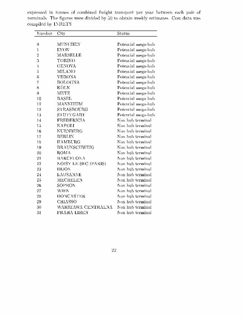
expressed in tonnes of combined freight transport per year between each pair of

terminals. The �gures were divided by 50 to obtain weekly estimates. Cost data was

compiled by INRETS.

Number City Status

0 MUNCHEN Potential mega-hub

1 LYON Potential mega-hub

2 MARSELLE Potential mega-hub

3 TORINO Potential mega-hub

4 GENOVA Potential mega-hub

5 MILANO Potential mega-hub

6 VERONA Potential mega-hub

7 BOLOGNA Potential mega-hub

8 K�OLN Potential mega-hub

9 METZ Potential mega-hub

10 BASEL Potential mega-hub

11 MANNHEIM Potential mega-hub

12 STRASBOURG Potential mega-hub

13 STUTTGART Potential mega-hub

14 FREDERICIA Non hub terminal

15 NAPOLI Non hub terminal

16 NURNBERG Non hub terminal

17 BERLIN Non hub terminal

18 HAMBURG Non hub terminal

19 BRAUNSCHWEIG Non hub terminal

20 ROMA Non hub terminal

21 BARCELONA Non hub terminal

22 NOISY LE SEC (PARIS) Non hub terminal

23 DIJON Non hub terminal

24 LAUSANNE Non hub terminal

25 MECHELEN Non hub terminal

26 SOPRON Non hub terminal

27 WIEN Non hub terminal

28 DONCASTER Non hub terminal

29 CHIASSO Non hub terminal

30 WARSZAWA CENTRALNA Non hub terminal

31 PRAHA LIBEN Non hub terminal

22