optimal foreign exchange intervention in an inflation...

Open Econ Rev (2014) 25:429–450DOI 10.1007/s11079-013-9287-3

RESEARCH ARTICLE

Optimal Foreign Exchange Intervention in an InflationTargeting Regime: Some Cautionary Tales

Matthew Canzoneri ·Robert Cumby

Published online: 23 October 2013© Springer Science+Business Media New York 2013

Abstract Devaluations and fiscal retrenchments coming from developed coun-tries are buffeting less developed countries. Many emerging market countries haveadopted inflation targeting as “best practice,” but now they are being advised toenhance their inflation targeting regimes with foreign exchange intervention. Herewe use a DSGE model to tell some cautionary tales about this advice. A Taylor ruleguides interest rate setting, while foreign exchange interventions are used as a secondtool of monetary policy. These interventions are effective in our model since domesticand key currency bonds are imperfect substitutes. We derive optimal (Ramsey) inter-vention policies in response to foreign devaluations and fiscal retrenchments, andfind that they are rather complex. So, we compare the optimal responses to policiesthat simply smooth real or nominal exchange rate movements. Our results suggestthat discretion may be the better part of valor: pure inflation targeting may comecloser to the optimal policy than exchange rate smoothing. A secondary result mayalso be of some interest: foreign exchange interventions have a stronger impact oninflation and output in an inflation targeting regime than do sterilized interventions;the Taylor rule augments the effects of a given intervention.

Keywords Foreign exchange intervention

JEL Classifications E5 · F3 · F4

We thank Mauricio Villamizer Villegas and especially Behzad Diba for helpful comments. But weare solely responsible for the contents of this paper.

M. Canzoneri (�) · R. CumbyGeorgetown University, Washington, DC, USAe-mail: [email protected]

R. Cumbye-mail: [email protected]

mailto:[email protected]

mailto:[email protected]

430 M. Canzoneri, R. Cumby

1 Introduction

Monetary and fiscal policies in the developed countries have responded to the greatrecession, and to fiscal imbalances, and these policy shocks are being felt in lessdeveloped countries. The loose monetary policies of the Fed, the ECB, the Bank ofEngland and the Bank of Japan have brought fresh accusations of currency wars;1

big fiscal retrenchments in the U.S. and Europe are on-again and off-again. Howare emerging market countries responding to these shocks? Many central banks haveeschewed their focus on exchange rate targeting and adopted inflation targeting astheir nominal anchor; this is now viewed as best practise. And indeed, there seemsto be a concern that public attention to movements in the exchange rate might betaken as a lack of commitment to the inflation target (although some central banksdo continue to intervene in foreign exchange markets).2

Advice now coming from IMF staff seems to be challenging this view: Blanchard(2012) explicitly advocates the use of foreign exchange intervention within an infla-tion targeting regime. Staff studies by Ostry et al. (2012a, b) and Benes et al. (2013)assume that interest rates are guided by a Taylor rule while foreign exchange inter-vention seeks to smooth real or nominal exchange rates around some medium runtarget. These studies generally conclude that these leaning against the wind policiescan be helpful in minimizing inflation and output fluctuations.

In this paper we use a DSGE model to tell cautionary tales about this enhancedinflation targeting regime. In our model, the central bank’s interest rate is guided bya Taylor rule while optimal (Ramsey) intervention policy seeks to maximize house-hold welfare. An inflation targeting central bank will indeed want to intervene, butthe optimal intervention policy proves to be rather complex; it would probably be dif-ficult for a central bank to implement. So, we also consider intervention policies thathave been observed in practise. An obvious alternative is to simply refrain from inter-vening; we will call this a pure inflation targeting regime. Other intervention policiesinvolve leaning against the wind: they seek to limit changes in either real or nominalexchange rates.

Our cautionary tales suggest that discretion may be the better part of valor: pureinflation targeting may be preferable to leaning against the wind unless an appropriateintermediate exchange rate target can be identified. And, there is no one intermediatetarget that is appropriate for all shocks coming from abroad. Finding an appropriateintermediate target and implementing a successful leaning against the wind policymay be as difficult as implementing the optimal policy. A final result that may beof some interest is that foreign exchange interventions within an inflation targetingregime have much bigger effects on inflation and output than sterilized interventionsof the same size; that is, the Taylor rule in an inflation targeting regime calls for

1For example, Brazilian Finance Minister Guido Mantega has made these charges repeatedly. See: “G20:Brazil Finance Minister: Currency Wars Have Become More Intense,” WSJ, Feburary 15, 2013.Theseconcerns are not restricted to developing counries. France, for example, has called for “medium-term”exchange rate targets, but the ECB has shown no inclination to respond.2See for example Blanchard (2012), Malloy (2013) or Villamizar-Villegas (2013).

Optimal Foreign Exchange Intervention in an Inflation Targeting Regime: Some Cautionary Tales 431

interest rate settings that augment the effects of the original intervention. These twointervention policies should not be conflated.

Foreign interventions must have a different effect than open market operations ifthey are to have an independent effect in an inflation targeting regime, and this will bethe case if home and foreign bonds are imperfect substitutes.3 The recent academicliterature has shied away from these issues. One reason for this is that currently pop-ular models almost invariably assume that bonds denominated in different currenciesare indeed perfect substitutes. In our model, the home country uses home bonds anda key currency bond (in addition to money) to facilitate trade, and as we shall see thismakes the two bonds imperfect substitutes.4 Our model has much in common withthe earlier portfolio balance models of Kouri (1976), Branson and Henderson (1985),and more recently Blanchard et al. (2005).

There is a very large literature pertaining to the general issues we discuss here.We are of course not the first to study the liquidity services of bonds. Early con-tributions to the literature include: Patinkin (1965), who put both money and bondsin the household utility function; and Friedman (1969), who discussed the optimumquantity of money and (private) bonds. More recent theoretical contributions include:Bansal and Coleman (1996), who used the approach to study the equity premiumpuzzle and related issues; Holmstrom and Tirole (1998), who argued that the pri-vate sector cannot satisfy its own liquidity needs when there is aggregate uncertainty;and Linnemann and Schabert (2010), who used a model similar to ours to studymacroeconomic policy.

Our basic assumption that government bonds provide liquidity should not be con-troversial. U.S. Treasuries facilitate transactions in a number of ways: they serveas collateral in many financial markets, and importers and exporters hold them astransaction balances. Empirical contributions to this literature include: Friedman andKuttner (1998), who studied the imperfect substitutability of commercial paper andU.S. Treasuries; Greenwood and Vayanos (2010), who find that the supply of long-term relative to short-term bonds is positively related to—and predicts—the termspread; and Krishnamurthy and Vissing-Jorgensen (2012), who find that the spreadbetween liquid treasury securities and less liquid AAA debt moves systematicallywith the quantity of government debt.

The rest of the paper proceeds as follows: In Section 2, we outline a two coun-try model suitable for studying foreign exchange intervention, and we illustrate thedifference between interventions conducted within an inflation targeting regime andsterilized interventions. In Section 3, we derive the optimal interventions in responseto monetary and fiscal policy shocks coming from abroad and compare them tointervention policies that lean against the wind; then we tell our cautionary tales. InSection 4, we conclude with a discussion of work for the future.

3The previously cited IMF staff papers discuss the empirical literature on the effectiveness of sterilizedinterventions. For a recent study, see Gagnon (2013).4Canzoneri et al. (2013b) used a similar structure to discuss empirical puzzles in the international financeliterature, and Canzoneri et al. (2013a) used a virtually identical structure to discuss the costs and benefitsof being a key currency country.


2 A Model of Foreign Exchange Intervention

Our model consists of a Home country (hereafter called “Home” ) and a Key Cur-rency country (hereafter called “KC” ). Bonds are imperfect substitutes for moneyin each country,5 and this fact alone would make Home and KC bonds imperfectsubstitutes. But, there is more: all trade is priced in units of the key currency. So,Home households use KC bonds to facilitate trade, and the Home government holdsKC bonds as official reserves for use in foreign exchange interventions. For simplic-ity, the two countries are symmetric apart for these two key currency assumptions.The fact that Home bonds are imperfect substitutes for KC bonds makes sterilizedinterventions effective in this model.

The rest of the model has standard NOEM features: Monopolistically competitivefirms produce an aggregate consumption good in each country; household consump-tion reflects habit formation and a bias for the domestically produced good; labor isthe only factor of production (there being no land or investment); the labor marketis competitive and wages are flexible, but prices are set in the staggered fashion ofCalvo.

2.1 The Model

In this section, we describe the model’s basic structure. We also describe how wesolve for the steady state and calibrate the model.

2.1.1 Households

We begin with the Home households. There is a continuum of Home households onthe unit interval. The utility of household h is

Uhousehold = E

∞∑

t=0

βt[log(ct (h)− ξct−1)− (1 + χ)nt (h)

1+χ]

(1)

where ct (h) is consumption of a composite final good (defined below), nt (h) is hoursof work, ct−1 is aggregate consumption last period, the parameter ξ is a measure ofhabit persistence, and the parameter χ is the inverse of the Frisch elasticity of laborsupply. Households are identical in equilibrium; so, we can dispense with householdindices. The household’s budget constraint, in units of the Home consumption good,is 6

mt + bt + bKC,tqt + (1 + τt )ct = (2)

wtnt +(mt−1 + Rt−1bt−1 + R∗

t−1bKC,t−1qt)/�t − xt + (1 − s)divH,t

5Canzoneri et al. (2008) present a closed economy model with banks, bank deposits and bank loans. Here,due to the complexity of the two country model, we take a less structural approach.6A note on notation: H and KC subscripts will be used to denote Home and KC assets and products whenthose bonds or products are used in both countries; Home money and bonds, for example, are not held byforeign entities, and therefore they need no subscript. Supercript *’s will denote KC household demandsand supplies of assets and products; they will also denote KC interest rates, inflation rates, and velocity.


Home households hold Home money, mt , Home bonds, bt , and KC bonds, bKC,t ,to finance their purchases; τtct is a transactions cost which will be described later;wt is the competitive market wage; Rt−1 is the gross nominal interest rate on Homebonds; �t = Pt/Pt−1 is the gross rate of Home CPI inflation; xt is a lump sum tax;divH,t are dividends from Home firms and s is the share of Home equity held by KChouseholds;7 and finally qt is the real exchange rate (Home consumption goods perKC consumption good).

Following Schmitt-Grohe and Uribe (2004), we assume that transactions costsare proportional to consumption, and the factor of proportionality is an increasingfunction of velocity, νt :

τt = A(νt − υ)2

νtfor νt > υ

and τt = 0 for νt ≤ υ (3)

where υ is the satiation level of velocity and A is a cost parameter. The new elementhere is in our definition of velocity:

νt = ct

mt

(4)

where effective transactions balances–mt–are a Cobb-Douglass aggregate of moneyand bonds:

mt = mω1t b

ω2t (qtbKC,t )

ω3 (5)where 0 < ω1, 0 < ω2, 0 < ω3 and ω1 + ω2 + ω3 = 1; ω3 measures the importanceof KC bonds in the Home household’s transactions.

The Home household’s first order conditions include:

(ct − ξct−1)−1 = λt [1 + 2A(νt − υ)] (6)

1 −A(ν2t − υ2

)ω1(mt/mt ) = βEt [(λt+1/λt )/�t ] ≡ 1/Rt (7)

1 −A(ν2t − υ2

)ω2(mt/bt ) = RtβEt [(λt+1/λt )/�t ] ≡ Rt/Rt (8)

1 −A(ν2t − υ2

)ω3(mt/qt bKC,t ) = RtβEt [(λt+1/λt )(qt+1/qt )(1/�t)] (9)

where λt is the marginal value of wealth. We can price a bond that does not pro-vide liquidity services and call it the CCAPM bond; its gross return is Rt . Rt/Rt isless than one, reflecting the non-pecuniary return on Home bonds. (6) defines themarginal value of wealth. When real resources are depleted in the purchase of con-sumption goods, the marginal value of wealth is less than the marginal utility ofconsumption. (7) and (8) are the first order conditions for money and Home bonds;(9) is the first order condition for KC bonds.

7We do not model the equities market. We simply assume that each household owns a proportionate shareof the steady state Home country portfolio (of bonds and equity). The size and composition of this portfoliowill be calibrated so that KC earnings on Home equity balance Home earnings on KC bonds in the steadystate.


Since Home and KC bonds are not perfect substitutes, this model departs from theusual UIP condition. Equations (8) and (9) determine the substitutability of Homeand KC bonds. Linearizing around the steady state (which is described below) weobtain,

Rt −[R∗t + Et(et+1 − et )

]=

(ω3

ω2

)(S

R

)[bt − (qt + bKC,t )

](10)

where e is the nominal exchange rate, S is the steady state spread between theCCAPM rate and the government bond rate, R, and hats ( ˆ) denote percentage devi-ations from a steady state value. Note that if the interest rates, Rt and R∗

t , are heldconstant, a change in the relative supply of Home and KC bonds requires a change inthe nominal exchange rates. This fact will be important in our discussion of monetarypolicy.

KC households are modeled symmetrically, but with one major exception: KChouseholds do not use foreign bonds to finance their purchases. Their transactionscosts are again proportional to consumption:

τ ∗t = A∗(ν∗t − υ∗)2

νtfor ν∗t > υ∗ (11)

and τ ∗t = 0 for ν∗t ≤ υ∗

and

ν∗t = c∗tm∗

t

(12)

But effective transactions balances – m∗t – are a Cobb-Douglass aggregate of KC

money and KC bonds:

mt =(m∗

t

)ω∗1(b∗KC,t

)ω∗2 (13)

where 0 < ω∗1, 0 < ω∗

2, and ω∗1 + ω∗

2 = 1.

2.1.2 Firms, Key Currency Pricing, Intermediate Goods, Final Goods

We model monopolistic competition in a standard way; so, our description of it can bebrief, focusing on aspects that are specific to our model. In each country, a continuumof monopolistically competitive firms hire workers on a competitive labor marketand produce a continuum of intermediate goods using a common linear technology.Intermediate goods firms in each country price their goods in the staggered mannerof Calvo; the Calvo parameters are set so that average price duration is four quarters.

There is, however, an important asymmetry in the price setting. KC firms set theirprices in terms of their own currency, both for goods sold at home and for goods thatare exported; the law of one price holds for KC goods. Home firms set their pricesin terms of their own currency for good sold domestically, but they set their prices interms of the key currency for goods exported to KC.

The Home and KC national products, yH,t , and y∗KC,t are CES aggregates of theintermediate goods, with elasticity of substitution ζ . The final Home consumption


good (appearing in the utility function (1)) is a CES aggregate of Home consumptionof the Home product, cH,t , and Home consumption of the KC product, cKC,t :

ct =[μ1/η(cH,t )

(η−1)/η + (1 − μ)1/η(cKC,t )(η−1)/η

]η/(η−1)(14)

where 1/2 < μ < 1. The parameter μ measures the degree of “home bias”in consumption. The final KC consumption good, c∗t , is defined in an analogousmanner.

2.1.3 Equilibrium Conditions

Most of the market equilibrium conditions are obvious. Here, we focus on those aboutwhich there may be some confusion. The equilibrium condition for KC bonds is:

d∗t − b∗KC,t = bKC,t + bGKC,t (15)

where d∗t is the total supply of KC bonds issued by the KC government and bGKC,t

are the KC bonds held by the Home central bank. The KC bonds that are not heldby KC households (the LHS of the equilibrium condition) must be held by Homehouseholds or the Home central bank (the RHS).

Government spending falls on the domestic good in each country, so the outputequilibrium conditions are:

yH,t = (1 + τt )cH,t + gt + (1 + τ ∗t )c∗H,t

y∗KC,t = (1 + τ ∗t )c∗KC,t + g∗t + (1 + τt )cKC,t (16)

2.1.4 The Steady State and Model Calibration

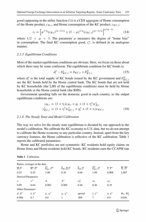
The way we solve for the steady state equilibrium is dictated by our approach to themodel’s calibration. We calibrate the KC economy to U.S. data, but we do not attemptto calibrate the Home economy to any particular country. Instead, apart from the keycurrency features, the Home calibration is reflective of the KC calibration. Table 1reports the calibrated parameters.

Home and KC portfolios are not symmetric: KC residents hold equity claims onHome firms and Home residents hold KC bonds. KC residents earn the CCAPM rate

Table 1 Calibration

Ratios, averages in the data

m/c m∗/c∗ b∗KC/c

∗ bKCq/c bH /c bG

KC/c τ , τ ∗ �,�∗

0.25 0.25 1.00 0.36 0.64 1.09 0.008 1.007

Derived Parameters

υ υ∗ A A∗ ω∗1 ω1 ω2

0.99 0.64 0.003 0.005 0.46 0.46 0.35

Other Parameters

β, β∗ ξ, ξ∗ μ,μ∗ χ, χ∗ spread ζ, ζ ∗ η, η∗ d, ∗d

0.988 0.7 0.8 1 .005 7 0.9 0.036


on their Foreign equity claims, while Home residents earn the liquid bond rate ontheir KC bond holdings. Since liquid assets command a liquidity premium, KC earnsa higher rate of return on its foreign assets than it pays on its foreign liabilities. KCis a net debtor, but the difference in the rates of return is sufficient in the steady stateto balance the income receipts and payments. So, the current account is balanced inthe steady state.

Canzoneri et al. (2013b) provides a discussion of data sources and estimationprocedures for the parameters that we have estimated, including the shock pro-cesses described below. A number of other parameters reported in Table 1 havestandard values taken from the literature. But our model has a number of parame-ters (those in our specifications of transactions costs and the transactions technology)that we cannot pin down in a standard way. We set �∗, R∗, and the ratios reportedin the first panel of Table 1 using data, and we set transactions costs to 0.8 % ofconsumption. We then use the ratios in the steady state equations to back out theparameters reported in the second panel of Table 1, and calculate the relevant steadystate values of some other variables along the way.

Specifically, we have R∗ = �∗/β; we set R = R∗,� = �∗, and q = 1, by sym-metry. We then solve the Home household’s optimality conditions (7), (8) and (9) toeliminate the terms involving velocity and calculate the values of ω1, ω2 and ω3 thatare consistent with the values of asset holding ratios found in Table 1. Similarly, weuse the corresponding KC household’s optimality conditions to infer the values of ω∗

1and ω∗

2. Next, we use the equations defining velocity and effective transactions bal-ances to calculate the steady state values of velocity terms that are consistent with ourasset holding ratios and the values of ω1, ω2, ω3, ω∗

1 and ω∗2. We then solve (3) and

(8), and their KC counterparts, for the satiation levels of velocity and the parametersA and A∗ in our specification of transactions costs. Given these parameter values, therest of our steady state calculations are standard—the real wage is pinned down bythe firms’ optimality condition, we can calculate employment from the labor-leisuremargin, and so on.

2.1.5 Fiscal Policy

The Home government’s flow budget constraint is

mt+bt−bGKC,tqt+R∗t−1b

GKC,t−1qt /�

∗t = pH,tgt−xt+(mt−1+Rt−1bt−1)/�t (17)

Home government spending, gt , falls entirely on Home output; pH,t is the price ofHome goods relative to the price of the Home consumption good.

We assume Home government spending is held constant; that is, gt = g, wherebars indicate steady state values. Lump sum taxes, xt , assure fiscal solvency:

xt − x = ϕ(bt − b

)(18)

where ϕ is greater than the steady state real rate of interest on government bonds.Fiscal policy is “Ricardian” in the sense of Woodford (1995), or “passive” in the senseof Leeper (1991). However, the model is non-Ricardian in the traditional sense. Why?Government bonds provide liquidity services, so the government borrowing rate, Rt ,


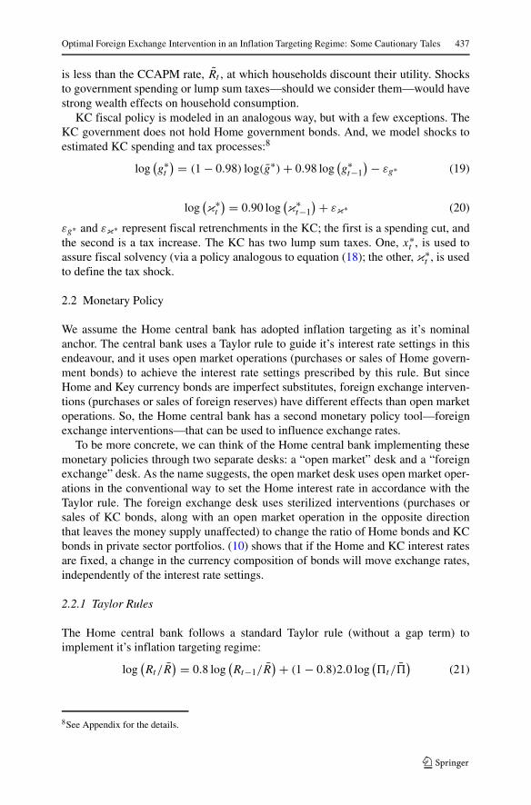
is less than the CCAPM rate, Rt , at which households discount their utility. Shocksto government spending or lump sum taxes—should we consider them—would havestrong wealth effects on household consumption.

KC fiscal policy is modeled in an analogous way, but with a few exceptions. TheKC government does not hold Home government bonds. And, we model shocks toestimated KC spending and tax processes:8

log(g∗t

) = (1 − 0.98) log(g∗)+ 0.98 log(g∗t−1

) − εg∗ (19)

log(κ∗t

) = 0.90 log(κ∗t−1

) + εκ∗ (20)

εg∗ and εκ∗ represent fiscal retrenchments in the KC; the first is a spending cut, andthe second is a tax increase. The KC has two lump sum taxes. One, x∗t , is used toassure fiscal solvency (via a policy analogous to equation (18); the other, κ∗

t , is usedto define the tax shock.

2.2 Monetary Policy

We assume the Home central bank has adopted inflation targeting as it’s nominalanchor. The central bank uses a Taylor rule to guide it’s interest rate settings in thisendeavour, and it uses open market operations (purchases or sales of Home govern-ment bonds) to achieve the interest rate settings prescribed by this rule. But sinceHome and Key currency bonds are imperfect substitutes, foreign exchange interven-tions (purchases or sales of foreign reserves) have different effects than open marketoperations. So, the Home central bank has a second monetary policy tool—foreignexchange interventions—that can be used to influence exchange rates.

To be more concrete, we can think of the Home central bank implementing thesemonetary policies through two separate desks: a “open market” desk and a “foreignexchange” desk. As the name suggests, the open market desk uses open market oper-ations in the conventional way to set the Home interest rate in accordance with theTaylor rule. The foreign exchange desk uses sterilized interventions (purchases orsales of KC bonds, along with an open market operation in the opposite directionthat leaves the money supply unaffected) to change the ratio of Home bonds and KCbonds in private sector portfolios. (10) shows that if the Home and KC interest ratesare fixed, a change in the currency composition of bonds will move exchange rates,independently of the interest rate settings.

2.2.1 Taylor Rules

The Home central bank follows a standard Taylor rule (without a gap term) toimplement it’s inflation targeting regime:

log(Rt/R

) = 0.8 log(Rt−1/R

) + (1 − 0.8)2.0 log(�t/�

)(21)

8See Appendix for the details.


where the steady state inflation rate, �, is the central bank’s inflation target. The KCcentral bank follows an analogous rule:9

log(R∗t /R

∗) = 0.8 log(R∗t−1/R

∗) + (1 − 0.8)2.0 log(�∗

t /�∗) − εR∗ (22)

where εR∗ is a cut in the KC policy rate. Since the Taylor rule is highly inertial, thisshock produces a very persistent decrease in the KC policy rate, which would in turncreate a persistent depreciation of the KC exchange rate.

2.2.2 A Home Foreign Exchange Intervention

Here, we describe the short run effects of a very persistent sale of foreign reserves:10

log(bGKC,t

)= (1 − 0.95) log

(bGKC

)+ 0.95 log

(bGKC,t−1

)− εb∗ (23)

Figure 1a illustrates the basic effects of this foreign exchange intervention. The saleof foreign reserves causes a real appreciation, which in turn lowers Home inflationand decreases Home output.

It is important to recognize that the effects of a foreign exchange interventiondepend crucially upon what the Home central bank is doing with its open marketoperations and the interest rate. In Fig. 1a, the central bank is using open marketoperations to make the policy rate consistent with it’s Taylor rule (21); that is, theintervention is conducted within an inflation targeting regime.

Alternatively, the central bank could use it’s open market operations to “sterilize”the foreign exchange intervention (that is, hold the Home money supply constant); inthis case, interest rates will follow a very different path. The dashed lines in Fig. 1bshow the effects of a sterilized intervention of the same size; here, both the Homeand Foreign central banks are using open market operations to make their nominalmoney supplies grow at the steady state rate of inflation.

For better or worse, a given sale of foreign reserves has a greater impact on infla-tion and output in an inflation targeting regime. The intervention policies we discussin the next section should not be confused with sterilized interventions; the distinctionis important quantitatively. We turn next to optimal foreign exchange interventionwithin an inflation targeting regime.

3 Intervention Policies

In this section, we derive the Ramsey response to policy shocks coming from devel-oped economies, or in our simple two country framework, the KC.11 The first shockis a sustained decrease in the KC policy rate; this creates a sustained depreciation of

9The parameters in the interest rate rule are chosen to conform with standard estimates of the U.S. Taylorrule.10The parameters in this AR(1) process are actually taken from a regression of official holdings of U.S.treasury bonds.11The calibration of these shocks is discussed (Canzoneri et al. 2013b)


Fig. 1 a Foreign reserve sale (within the contex of inflation targeting). b Foreign reserve sale


the KC currency (unless of course the Home central bank does something to thwartit). The second shock is a sustained decease in KC government spending, and thethird is a sustained increase in KC taxes. The final shock is combination of all threeshocks: a one standard deviation cut in the policy rate, a one standard deviation cutin government spending, and a one standard deviation increase in taxes. 12

As we shall see, the Ramsey responses are rather complex; implementing a Ram-sey policy may be beyond the capability of central banks in practise. So, for eachshock coming from the KC, we will consider three alternative policies that have actu-ally been used in practise. The first is to simply do nothing; that is, the Home centralbank sticks to pure inflation targeting, as defined by its Taylor rule. The second andthird alternatives are leaning against the wind policies. One is to smooth nominalexchange rate movements; more specifically, foreign exchange interventions limit thestandard deviation of changes in the nominal exchange rate to half of what it wouldbe with pure inflation targeting. The other is to smooth real exchange rate move-ments; the standard deviation of changes in the real exchange rate is limited to halfof it would be with be with pure inflation targeting. In each case, the exchange rate issmoothed around its long run equilibrium value. A vast empirical literature is devotedto estimating these equilibrium values; so, we will assume that these interventionpolicies would indeed be implementable.

First however, we must discuss how we select the steady state level of foreignreserves. On the one hand, the Home government would like to sell all of its KCbonds—or even go negative in them if that were allowed—because they pay less thanthe CCAPM bond (which has no liquidity value); on the other hand, the Home centralbank needs foreign reserves to conduct its intervention policy. It is beyond the scopeof the present paper to calculate the optimal steady state level of reserves. Instead,we assume that the Ramsey planner maximizes

URamsey = Uhousehold + κE

∞∑

t=0

βt log(bGKC,t

)(24)

where Uhousehold was defined in equation (1). We set κ at a very small number(0.001); so, the Ramsey planner is basically maximizing household utility.

In describing the various intervention policies, we will focus our attention on twoof the factors that the planner generally has to trade off: getting the right balancebetween labor and leisure, and minimizing fluctuations in the aggregate price level.13

Since firms’ production is linear in labor, output is synonymous with work effort inthe impulse response functions analyzed in the next section.14 Our focus on inflationand output volatility is similar to that in many official studies of intervention policy,

12The standard deviations come from estimates of stochastic processes for U.S. government spending,taxes, and the U.S. Taylor rule. See Canzoneri et al. (2013b)13With staggered price setting, fluctuations in the aggregate price level cause a dispersion of intermediategoods’ prices that distorts household consumption decisions; see Woodford (2003).14Staggered price setting creates a distortion between aggregate output and the aggregate work effort.However, the distortion is second order; so, it does not show up in impulse functions derived from thelinearized model.


and monetary policy more generally.15 Note however, that our Ramsey planner isconcerned with the household’s labor-leisure balance, and is not trying minimizeoutput fluctuations per se. This fact drives many of our results.

Our purpose here is to derive the Ramsey response to the foreign shocks describedabove and to compare its medium run effects with those of the alternative interventionpolicies; we take the medium run to be four years (or sixteen quarterly periods).

3.1 Responses to a Foreign Depreciation

The solid lines in Fig. 2a show the optimal response to a sustained cut in the KCpolicy rate. The dashed lines show what would happen if the Home central bank stuckto pure inflation targeting. We begin with the latter.

With no intervention, the real exchange rate appreciates, as would be expected,but Home output rises. This may sound contradictory, and indeed in a symmetricversion of our model, Home output falls (at least initially).16 Several factors limitthe output decrease in either version of our model: First, KC income rises and thiscreates demand for the Home good, partially offsetting the relative price effect. Andsecond, the real appreciation lowers the price of KC goods, and this is deflationaryin the initial period; that is, the Taylor rule implies that Home nominal (and real)interest rates fall. In the present version of our model, there is also a third factor. Theappreciation increases the real value of Home households’ stock of KC bonds; thiscreates a strong non-Ricardian wealth effect on Home consumption, and adding thislast factor eliminates the decrease in output altogether.

The optimal foreign exchange intervention is for the Home central bank to buy KCbonds. As explained in Section 2, this has an expansionary effect on inflation and out-put. In other words, pure inflation targeting results in too little work and not enoughconsumption; the optimal intervention seeks to correct this imbalance. So, both theTaylor rule and the optimal intervention are expansionary, and to an extent that theyactually destabilize output. This intervention policy also smooths fluctuations in theinflation rate, reducing the relative price distortion created by staggered price setting.

It would appear, however, that the outcomes for inflation and output under thesetwo policies are not too dissimilar, at least over the first six or eight quarters. TheRamsey policy is of course the best policy, but it may be impractical to implement.Can a leaning against the wind policy do better than pure inflation targeting?

Figure 2b compares the optimal intervention policy with the two policies of lean-ing against the wind. Reducing the volatilities of nominal or real exchange ratechanges by half requires large purchases of KC bonds; these interventions are muchlarger than is optimal. And the paths of the real exchange rate are far from optimal,especially for real exchange rate smoothing.

Maintaining “competitiveness” is the usual concern in a currency war, but poli-cies of smoothing relative prices around their long run values would not seem to be

15See for example the recent intervention studies of Ostry et al. (2012a) and Benes et al. (2013)16In the symmetric version, Home households do not use KC bonds for transactions purposes or price theirexports in terms of the key currency.


Fig. 2 a, b Foreign interest rate decrease


appropriate in this regard. When competitiveness is evaluated with the labor-leisuredecision in mind, it is not synonymous with relative price smoothing.

Nominal exchange rate smoothing results in a output path that is relatively closeto optimal; moreover, inflation fluctuations are almost eliminated. Real exchangerate smoothing appears to do rather poorly—there is not nearly enough work effortafter the second period and too much leisure. In addition, inflation fluctuates widely,which increases relative price dispersion and lowers welfare. Pure inflation target-ing certainly seems preferable to real exchange rate smoothing in response to a lowinterest rate policy coming from abroad.

3.2 Responses to Foreign Fiscal Retrenchments

Fiscal retrenchments can come in the form spending cuts or tax hikes, or some combi-nation of the two. We have assumed that taxes are non-distortionary, but even a lumpsum tax increase will lower aggregate demand in our model since it is non-Ricardian.As explained earlier, household wealth effects play a large role in our model, andfiscal retrenchments—at home or abroad—can have a strong impact on consumptionand output.

3.2.1 A Foreign Government Spending Cut

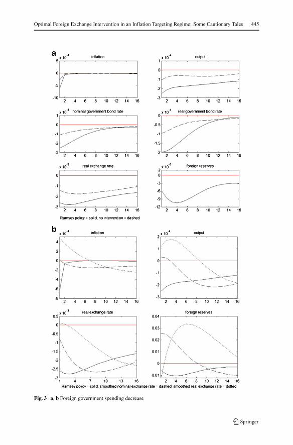
The solid lines in Fig. 3a show the optimal response to a sustained decrease KCgovernment spending, and the dashed lines show what would happen if the Homecentral bank stuck to pure inflation targeting. As before, we begin with this case.

With no intervention, the KC spending cut decreases the demand for KC goods,causing the Home real exchange rate to appreciate. This in turn decreases Homeinflation and output. But once again, the initial effect on the real exchange rate isattenuated by several factors: The first is nominal price rigidity, which slows relativeprice adjustments. And the second is the Home central bank’s inflation targeting; itsTaylor rule calls for a decrease in interest rates, which limits the nominal and realappreciations.

The KC spending cut is a relative demand shock, and efficiency requires a rel-ative price adjustment. Price rigidities and inflation targeting get in the way ofthis. Output and the work effort do not fall enough. Once again the labor-leisuremargin is out of balance; households are off their labor supply curve because ofprice rigidity.

The optimal foreign exchange intervention is to sell KC bonds, causing the realexchange rate to appreciate more, and bringing the labor-leisure margin more intobalance. The optimal policy is not to stabilize output, but to push it further down.Both inflation and output fall more, and the Taylor rule calls for an even biggerdecrease in interest rates. It is interesting to note that inflation targeting and for-eign exchange intervention are taking opposite stances in this case. The Taylorrule calls for inflationary interest rate setting, while the optimal intervention policycalls for deflationary foreign bond sales. Inflation credibility (the inflation target-ing) and optimal stabilization (the optimal intervention policy) are at odds with oneanother.


Figure 3b compares the optimal intervention policy with the two policies of lean-ing against the wind. Reducing the volatilities of nominal and real exchange ratechanges by half requires large purchases of KC bonds. These interventions go in theopposite direction of the optimal interventions. Leaning against the wind does tend tostabilize output, but once again, that is not the best thing to do. In addition, inflationfluctuations are large compared to their optimal path.

The basic message here is that efficient adjustment to real shock requires achange in relative prices. Stabilizing exchange rates around their long run equi-librium values appears to be counterproductive. Comparing Figs. 3a and b, pureinflation targeting would seem preferable to the leaning against the wind poli-cies.

3.2.2 A Foreign Tax Increase

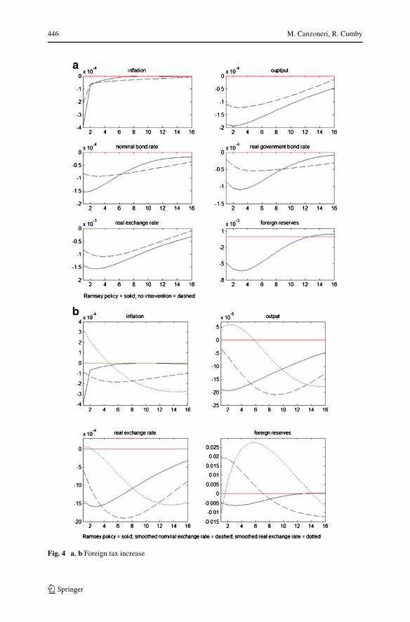
Figures 4a and b show the various policy responses to a sustained increase in KCtaxes, and they tell much the same story as the spending cut. The KC consumerhas a home bias for the KC good, so the tax hike decreases the relative demandfor KC goods. The efficient adjustment to this shock requires a change in relativeprices. For the reasons given above, the real appreciation under pure inflation target-ing is insufficient. And the optimal intervention is to sell reserves, amplifying thereal appreciation. Once again, intervention policy works to undo the damage done byinterest rates under inflation targeting.

Intervention policies that lean against the wind are counter productive: they go thewrong way. Comparing the two figures, pure inflation targeting seems preferable toleaning against the wind.

3.3 Responses to a Depreciation and a Fiscal Retrenchment

Figure 5a and b show the policy responses to a combination of shocks coming fromabroad: the KC interest rate is lowered by one standard deviation, KC governmentspending is cut by a standard deviation, and KC taxes are increased by a standarddeviation. The solid lines in Fig. 5a show the optimal response, and the dashed linesshow the response to pure inflation targeting. The results are of course a kind ofaveraging of the three previous exercises.

With this combination of shocks, the shape of the paths for inflation and outputlook like those in Fig. 2a for a KC interest rate cut. However, the policy prescriptionfor foreign exchange intervention looks more like those in Figs. 3a and 4a for fis-cal retrenchments. The central bank sells reserves to increase the real exchange rateappreciation, and decrease the work effort. And once again, inflation targeting andforeign interventions work in opposite directions: since inflation and output fall ini-tially, the Taylor rule calls for an inflationary policy, while the optimal interventionpolicy is deflationary.

Figure 5b shows that the optimal intervention is relatively modest, while theleaning against the wind policies require massive interventions and in the wrongdirection. Pure inflation targeting seems preferable to leaning against the wind forthis combination of shocks.


Fig. 3 a, b Foreign government spending decrease


Fig. 4 a, b Foreign tax increase


Fig. 5 a, b Foreign depreciation and fiscal retrenchment


4 Leaning Against the Wind: cautionary tales

The last section offered some cautionary tales about intervention policies that leanagainst the wind when external events cause exchange rates to fluctuate. Smoothingreal exchange rate movements seems to be particularly problematic. In many cases,pure inflation targeting—or refraining from intervening—seemed the better part ofvalor.

The advantage of the leaning against the wind policies is that they are imple-mentable in practise. All they require is an estimate of the long run equilibrium valueof the real (or nominal) exchange rate, and there has been considerable effort put intoobtaining such estimates. By contrast, the Ramsey policies described here are quitecomplex and are probably not implementable.

The problem is that efficient adjustment to real shocks requires movements inrelative prices, at least in the short to medium run;17 the real exchange rate canaccommodate some of the real consequences of changes in relative supplies anddemands if it is allowed to move. Moreover, with price rigidities, the same is true formonetary shocks, such as the foreign depreciation considered above.

To be fair, most of those who advocate leaning against the wind policies wouldprobably not characterize them as we have here. They advocate smoothing real ornominal exchange rate movements around “intermediate” targets, not a long runvalue. We have not tried to derive operational intermediate targets because it is notclear how one would do so. For one thing, there is no single intermediate targetfor either the nominal or the real exchange rate. The appropriate intermediate targetdepends upon the shock, or combination of shocks, that is causing the exchange rateto move. These leaning against the wind policies might be as complex as the Ramseypolicy.

Of course, pure inflation targeting requires none of this; it is operational. The realquestion for central banks is if they think they have enough information to intervenesuccessfully. Once again, discretion may be the better part of valor.

5 In Conclusion

We have already summarized our main conclusions in the last subsection. Inconcluding, we will discuss two topics that might be worth pursuing in future work.

Our cautionary tales suggest that smoothing exchange rate movements around pre-viously estimated long run equilibrium values may not be a good idea. Smoothingaround a state (or shock) dependent intermediate target may be an effective policy.The problem of course is in identifying the appropriate target. This project seemswell worth pursuing, especially at central banks that want to implement the enhancedinflation targeting regime advocated recently by IMF staff.

17If the shocks are not stationary, the long run real exchange rate will also be affected. The shocks weconsidered were all stationary.


Another issue is whether or not foreign exchange interventions have a differenteffect than open market operations, and if they do, why.18 As mentioned earlier, thereis an empirical literature suggesting that they do, but the answer is still controver-sial. We have made home and foreign bonds imperfect substitutes in our model byassuming that they both facilitate trade. If however they are imperfect substitutes forsome other reason—say risk premia, or capital market imperfections—then foreignexchange interventions could have very different effects than what we obtain in ourmodel. All of this suggests that model uncertainty should be taken into account ifa central bank is serious about trying to implement the enhanced inflation targetingregime.

There is literature on robust control that incorporates model uncertainty into policyevaluation.19 In particular, this literature tries to develop policy rules that are robustto model misspecification. In our case, bonds may not even be imperfect substitutes,or they may be imperfect substitutes in a different way, or to a different degree, thanwas modeled. Applying these techniques to the issues discussed here would seemmost appropriate.

References

Benes J, Berg A, Portillo R, Vavra D (2013) Modeling sterilized interventions and balance sheet effects ofmonetary policy in a new-keynesian framework. IMF Working Paper, WP/13/11

Bansal R, Coleman WJ (1996) A monetary explanation of the equity premium, term premium, and risk-free rate puzzles. J Polit Econ 104(6):1135–1171

Blanchard O, Giavazzi F, Sa F (2005) Brook Pap Econ Act 1:1–49Blanchard O (2012) Monetary policy in the wake of the crisis. In: Blanchard O, Romer D, Spense M,

Stiglitz J (eds) Chapter 1 of in the wake of the crisis. MIT Press, CambridgeBranson W, Henderson D (1985) The specification and influence of asset markets. In: Jones R, Kenen

P (eds) Handbook of international economics II. Elsevier, AmsterdamCanzoneri M, Cumby R, Diba B, Lopez-Salido D (2008) Monetary aggregates and liquidity in a Neo-

Wicksellian framework. J Money Credit Bank 40(4):1667–1698Canzoneri M, Cumby R, Diba B, Lopez-Salido D (2013a) Key currency status: an exorbitant privilege and

an extraordinary risk, mimeo. J Int Money Financ 37:371-393Canzoneri M, Cumby R, Diba B (2013b) Addressing international empirical puzzles: the liquidity of

bonds. Open Econ Rev 24(2):197-215Friedman M (1969) The optimum quantity of money and other essays. Aldine Publishing Company,

ChicagoFriedman B, Kuttner KN (1998) Indicator properties of the paper-bill spread: lessons from recent

experience. Rev Econ Stat 80(1):34–44. MIT PressGagnon J (2013) The elephant hiding in the room: currency intervention and trade imbalances. Peterson

Institute for International Economics Working Paper Series, WP 13–2Giordani P, Soderlind P (2004) Solution of macromodels with hansen-sargetn robust policies: some

extensions. J Econ Dyn Control 28:2367–2397Greenwood R, Vayanos D (2010) Bond supply and excess bond returns. NBER Working Paper Series No.

13806Hansen L, Sargent T (2007) Robustness. Princeton University Press, PrincetonHolmstrom B, Tirole J (1998) Private and public supply of liquidity. J Polit Econ 106(1):1–40

18As explained earlier, home and foreign bonds must be imperfect substitutes if foreign exchangeintervention is to be an additional policy tool in an inflation targeting regime.19See Hansen and Sargent (2007) and Giordani and Soderlind (2004)


Kouri P (1976) Capital flows and the dynamics of the exchange rate. Institute for International EconomicStudies, Stockholm. Seminar Paper 67

Krishnamurthy A, Vissing-Jorgensen A (2012) The aggregate demand for treasury debt. J Polit Econ12(2):233–267

Leeper E (1991) Equilibria under active and passive monetary policies. J Monet Econ 27:129–147Linnemann L, Schabert A (2010) Debt nonneutrality, policy interactions, and macroeconomic stability. Int

Econ Rev 51(2):461–474Malloy M (2013) Factors influencing emerging market central banks’ decision to intervene in foreign

exchange markets. IMF Working Paper, WP 13/70Ostry J, Ghosh A, Chamon M (2012a) Two targets, two instruments: monetary and exchange rate policies

in emerging market economies. IMF Staff Discussion Note, SDN/12/01Ostry J, Ghosh A, Chamon M (2012b) On inflation targeting and forex intervention: are two targets better

than one? VOXz, 27, MayPatinkin D (1965) Money, interest and prices: an integration of monetary and value theory, 2nd edn. Harper

& Row, New YorkSchmitt-Grohe S, Uribe M (2004) Optimal fiscal and monetary policy under sticky prices. J Econ Theory

114:198–230Villegas MV (2013) Identifying the effects of monetary policy shocks: fear of floating under inflation

targeting. Georgetwn University, dissertation chapterWoodford M (1995) Price level determinacy without control of a monetary aggregate. Carnegie Rochester

Conf Ser Public Policy 43:1–46Woodford M (2003) Interest and prices: foundations of a theory of monetary policy. Princeton University

Press, Princeton

optimal foreign exchange intervention in an inflation...

Documents