optimal design of supply chain network: a case study in

OPTIMAL DESIGN OF SUPPLY CHAIN NETWORK: A

CASE STUDY IN TOOTHBRUSH INDUSTRY

BY

TAI PHAM

A THESIS SUBMITTED IN PARTIAL FULFILLMENT OF

THE REQUIREMENTS FOR THE DEGREE OF MASTER OF

ENGINEERING (LOGISTICS AND SUPPLY CHAIN SYSTEMS

ENGINEERING)

SIRINDHORN INTERNATIONAL INSTITUTE OF TECHNOLOGY

THAMMASAT UNIVERSITY

ACADEMIC YEAR 2015

ii

Abstract

OPTIMAL DESIGN OF SUPPLY CHAIN NETWORK: A CASE STUDY IN

TOOTHBRUSH INDUSTRY

by

TAI PHAM Bachelor of Engineering (Industrial Engineering), Ho Chi Minh City University of Technology, 2012

Supply chain management has long been a compass for every successful

business. Its long-term decision plays an important role in shaping the supply chain

structure, or design of supply chain network, which significantly affects supply chain

performance for prolong period. Since each industry has a unique set of characteristics

which evidently drive the design of supply chain network, a number of various models

have been formulated to meet the needs of such business contexts. Even though many

models have been proposed for manufacturing industry context, most of them are based

on the facility location model. The model tends to lead the supply chain network design

model to be complicated. Therefore, the purpose of this research is to propose an

alternative approach to formulate manufacturing network design problem. Features,

such as multi-echelon, multi-commodity, product’s structure, and manufacturing

process, are taken into consideration as characteristics of the studied environment.

Moreover, uncertainty factors are also integrated to the model by employing

possibilistic theory. Eventually in addition to the methodology, a case study in a

consumer product firm is used to demonstrate applicability of the suggested method.

Two models, deterministic and fuzzy, has been explored in the study and both of them

has demonstrated the validity of the proposed formulation method. Moreover, it is

shown that the fuzzy model outperforms its deterministic counterpart in term of cost

effectiveness.

Keywords: strategic supply chain planning, supply chain network design, network

flow, production network, fuzzy programming, optimization, mixed-integer linear

programming (MILP), uncertainty

iii

Acknowledgements

First and foremost, I would like to express my deep gratitude to my advisor,

Assoc. Prof. Pisal Yenradee, for his dedicated support of my study. This research would

have not been completed without him. His patience, motivation, enthusiasm, and

immense knowledge helped me overcome many obstacles and finish my thesis timely.

Besides my advisor, I would like to thank the rest of my thesis committee: Assoc. Prof.

Navee Chiadamrong and Asst. Prof. Teeradej Wuttipornpun, for their constructive

comments and overwhelming encouragement, but also for the challenged questions

leading to significant refinement of my work. Moreover, I also appreciate financial

support via EFS scholarship program provided by Sirindhorn International Institute of

Technology (SIIT), Thammasat University. Last but not least, I would like to thank my

parents for supporting me spiritually throughout the course of writing this thesis.

iv

Table of Contents

Chapter Title Page

Signature Page i Abstract ii Acknowledgements iii Table of Contents iv List of Tables vi List of Figures vii

1 Introduction 1

2 Literature Review 4

3 Methodology 10

3.1 Problem formulation 10

3.1.1 Conceptual Design 10

3.1.1.1 Processes and Products 10

3.1.1.2 Network Structure 11

3.1.2 Mathematical model development 12

3.1.2.1 Sets 12

3.1.2.2 Parameters 13

3.1.2.3 Decision variables 14

3.1.2.4 Objective function 15

3.1.2.5 Constraints 15

3.1.3 Model Tranformation 17

3.2 Case Study 18

3.2.1 Studied context 18

3.2.2 Description of input data 19

v

3.2.2.1 Locations 19

3.2.2.2 Products and processes 20

3.2.2.3 Supply sources 23

3.2.2.4 Demand origins 24

3.2.2.5 Transportation cost 26

3.2.3 Experimental design 26

4 Result and Discussion 27

4.1 Deterministic Scenario 27

4.2 Non-deterministic Scenario 29

4.3 Solution Comparison 31

5 Conclusions and Recommendations 35

5.1 Conclusion 35

5.2 Recommendations for further studies 35

References 36

Appendices 31

Appendix A Input Data 40

Appendix B OPL Model 62

vi

List of Tables

Tables Page

2.1 Summary of Supply Chain Network Problem 8

3.1 Locations’ yearly fuzzy cost – lOP 19

3.2 Detailed recipe of SKU C – ,R k l 20

3.3 Processes’ Capacity (in mil. of UOM) – ioCap 22

3.4 Process 1’s annualized fuzzy fixed cost ($) – ioSE 22

3.5 Process 1’s unit production cost of handle C ($/piece) – ikoP 23

3.6 Unit shortage cost of each SKU ($/SKU) – kUSC 23

3.7 Supplier data 24

3.8 Customer Demand (in thousands of units) – ikD 25

4.1 Total cost summary 27

4.2 Decision summary 28

4.3 Demand allocation 29

4.4 Objective values in each state 30

4.5 Constraint Summary 31

4.6 Fuzzy Solution’s Decision Summary 32

4.7 Fuzzy Solution’s Demand Allocation 33

vii

List of Figures

Figures Page

3.1 BOM tree 11

3.2 Process network 11

3.3 Network representation 12

3.4 BOM structure of SKU C 20

3.5 Toothbrush manufacturing process network 21

4.1 Plants' portfolio and configuration 28

4.2 Fuzzy Solution’s Product Portfolio and Configuration 32

1

Chapter 1

Introduction

Under tough pressure of competition on global playground and high expectation

from customer nowadays, businesses are pushed to pay more investment and focus on

managing their supply chains effectively. A supply chain is a network of facilities and

streams of commodities that flow among them. Those facilities are composed of

suppliers, manufacturing plants, warehouses, distribution centers, and retail premises,

while commodities comprise raw materials, work-in-process, and finished goods.

Supply chain management (SCM) defined by Simchi-Levi (2007) as “a set of

approaches utilized to efficiently integrate suppliers, manufacturers, warehouses, and

stores, so that merchandise is produced and distributed at the right quantities, to the

right locations, and the right time, in order to minimize systemwide costs while

satisfying service level requirements”. By this definition, it is indicated that SCM

involves activities at many levels ranging from strategic through tactical to operational

within a business. Chopra and Meindl (2007) described that strategic level aims at

determining the optimal structure or design of supply chain network. The addressed

decisions are about number, location, and size of warehouses and/or plants as well as

the connections among them. Both Watson, Lewis, Cacioppi, and Jayaraman (2012)

and Simchi-Levi (2007) demonstrated that such decisions at this level have a high

impact on supply chain performance since they are expensive and difficult to be

changed. It is discussed that roughly 80% of supply chain expenses are trapped in its

facilities which is equivalent to that of the cost kept in a product design. As a result,

strategic network planning – or supply chain network design (SCND) – has drawn much

attention from management and has required extensive research.

In different industrial contexts, Vila, Martel, and Beauregard (2006) argued that

nature of SCND problem has changed significantly. In retail or distribution context, the

main concerns are the movement of products and locations of facilities because flows

from origin to destination are identical. On the other hand, the stream is no longer

uniform in the context of manufacturing because most of the products are not simply

collected and transported. Instead, there are series of transformation activities which

2

are performed among production facilities to convert materials into a particular product.

Each product has its own recipe of materials and set of desired production stages. The

recipe of materials involves in supply side sourcing decisions, while the set of desired

production stages associates with capital decisions and configuration of the network.

Therefore, it is necessary to address impacts from not only movement of goods and

locations but production processes and product architectures in manufacturing-related-

network design problem.

Melo, Nickel, and Saldanha da Gama (2009) accomplished a thorough review

on development of optimization models which support supply chain management. They

revealed many studies that are related to manufacturing context. Most of those research

works had been developed and formulated based on classical facility location models

which are centered on facility decision. However, this approach makes the models more

complicated. This has provided a motivation to elaborate a novel approach which will

generate a more simplified model. In addition to the approach, another obstacle which

is very common to every strategic decision is that the future is always unpredictable.

Therefore, taking uncertainty into account is inevitable.

The purpose of the thesis is to introduce a new method to formulate the supply

chain network design problem in manufacturing industry. The problem encompasses

two decisions which are related to network structure and configuration. The first

decision is to determine number of locations, transportation links, supply sourcing, and

demand allocation, while the second one aims at identifying production process

network within each selected location. In addition, features, such as multi-echelon,

multi-commodity, product’s structure, and manufacturing process, are considered to

capture characteristics of manufacturing business. Besides, uncertainty is also

accounted for. Although probability theory has become popular in SCND by the mean

called stochastic programming, the drawback is that this method depends heavily on

past collected data to describe the future situation which might not actually be realized

accordingly. As a result, instead of using probability theory, possiblistic theory is

proposed to be used as a mean to dictate the future. An advantage of this theory is that

it does not require extensive efforts to collect data. Instead, experts’ experience and

management references are the inputs. However, since these inputs sometimes may not

yield a good result, it is reasonable to perform post hoc analysis to improve the result

3

intuitively by alternative methods. Finally, a case study of a toothbrush producer has

been employed to demonstrate the applicability of this method on modelling network

design problem in manufacturing industries.

The remaining of the thesis is organized as follows. Related literature is

reviewed in Chapter 2. Conceptual design, problem formulation, and experimental

design are presented in Chapter 3. The implementation of the experiment and its results

are discussed in Chapter 4. Finally, the conclusion from the research has been drawn in

Chapter 5.

4

Chapter 2

Literature Review

Supply chain network is defined as a set of facilities such as suppliers, plants,

distribution centers, and customers. All of them are linked by transportation routes

carrying raw material, semi-finished goods, and finished products. With increasing

competition and market uncertainty on global basis, supply chain management (SCM)

is getting more and more attention from many companies around the world as a key

competitive capability. Based on the length of time horizon, SCM decision levels has

been divided into strategic, tactical, and operational levels. Strategic decisions have a

long term effect on supply chain performance, since they involve determining number,

location and capacities of various types of facilities, or the flow of material in the

system. Such decisions require a large sum of capital investment, which is difficult to

recover once it is allocated. Also, those facilities tend to stay in operation for extended

periods of time from now which makes them vulnerable to be affected by external

factors. Any change which occurs during their life-time may turn a selected site from a

good choice to an undesirable one. Consequently, strategic supply chain planning has

become the most important part of SCM. It is the reason that this topic gains much

attention from academic researchers. The intention of this chapter is to review studies

in supply chain network design, especially in manufacturing area. At first, the

relationship between strategic SCM problem and facility location problem (FLP) has

been outlined. Secondly, basic extensions of FLP which were conducted to handle the

strategic SCM problem are examined. After that, special extensions for manufacturing

sector have been discussed. Finally, conclusion is drawn from the review to provide

supports for the proposed research.

Currently, terms such as network design, and supply chain network design

(SCND) are often used, in most cases, as strategic SCM. As SCND is concerned with

optimal number, location, and size of warehouses and/or plants, it is apparent to

recognize the connection between network design and FLP in which locations are

considered to be selected from a limited set of potential candidates in order to satisfy

customers. If it is the case that setup cost is not different among all sites, the problem

5

is defined as p-median problem with the objective of minimizing total travel distance

or cost of meeting customers’ requirements. Otherwise, it may be considered as

uncapacited facility location problem (UFLP). On the other hand, when capacity is

known in advance, UFLP is renamed as capacitated facility location problem (CFLP).

All above models have shared common characteristics that are single period,

deterministic parameters, single product, mono type of facility, and location-allocation

decisions. The FLP has provided a solid foundation for developing SCND models.

However, the FLP models contain only a fundamental decision, location-allocation, and

features which do not reflect complicated relationship involving different kinds of

decision and advanced characteristics. Therefore, many extensions should be included

to cope with complicated circumstances.

In practical networks as defined above, there exist many types of facility which

play various roles in the network such as supplier, plant, and warehouse. Each facility

has been grouped into sets, called layers or echelons, according to its specific function.

Those facilities are connected together in order to transport goods from origins to

destinations. Multi-echelon facilities appeared in Arntzen, Brown, Harrison, and

Trafton (1995), Karabakal, Günal, and Ritchie (2000), Tsiakis, Shah, and Pantelides

(2001), Vidal and Goetschalckx (2001), Jang, Jang, Chang, and Park (2002), Wouda,

van Beek, van der Vorst, and Tacke (2002), Yan, Yu, and Cheng (2003), Kouvelis and

Rosenblatt (2005), Wilhelm et al. (2005), Cordeau, Pasin, and Solomon (2006), Melo,

Nickel, and Saldanha da Gama (2006), Ommeren, Bumb, and Sleptchenko (2006), Vila

et al. (2006), and A. S. Zadeh, Sahraeian, and Homayouni (2014). In addition, there are

many studies considering multi-products in their supply chains. Since strategic

planning spans for long time horizon, there are motivations to introduce multi-periods

or stochastic components to represent either predictable changes over time or

uncertainty associated with parameters, respectively. Fleischmann, Ferber, and Henrich

(2006), Melo et al. (2006), Ulstein, Christiansen, Grønhaug, Magnussen, and Solomon

(2006), Vila et al. (2006), and A. S. Zadeh et al. (2014) focused on uncertainty

elements, while multi-time-segments was taken into account by Arntzen et al. (1995),

Tsiakis et al. (2001) and Ommeren et al. (2006).

Furthermore, a supply chain does not simply send the same product from one

end, suppliers, to the other end, customers. The raw materials have to undergo

6

transforming processes to become finished goods before being delivered to customers.

It is necessary to include product’s Bill of Materials (BOM) to represent the impacts of

product’s ingredients and production processes to supply chain on overall product cost,

ingredient sourcing constraints, finished-goods manufacturing, overall throughput

capacity, and key capital decisions. Arntzen et al. (1995), Tsiakis et al. (2001), Vidal

and Goetschalckx (2001), Jang et al. (2002), Wouda et al. (2002), Yan et al. (2003),

Kouvelis and Rosenblatt (2005), Wilhelm et al. (2005), Cordeau et al. (2006),

Fleischmann et al. (2006), Vila et al. (2006), and A. S. Zadeh et al. (2014) took this

issue into consideration.

The most important extension is the inclusion of typical supply chain decisions,

which are capacity, production, and procurement. In traditional location problem,

capacity is usually assumed either unlimited or fixed amount. However, this assumption

is not held in contemporary supply chain settings because capacity is influenced by

several constraints such as budget, technology and so on. Therefore, many studies have

included this decision. Melo et al. (2006) and Vila et al. (2006) concurrently considered

capacity reduction and expansion over planning horizon. Melo et al. (2006), Ommeren

et al. (2006), Ulstein et al. (2006), and Vila et al. (2006) addressed setting up modules

which are pre-defined sizing. Combining capacity with choice of equipment and/or

technology has been handled by Arntzen et al. (1995), Mazzola and Neebe (1999),

Karabakal et al. (2000), Verter and Dasci (2002), Ulstein et al. (2006), and Vila et al.

(2006). The participation of multi-commodities feature in FLP has led to the need of

determining which product should be produced in which plant with which quantity. It

is the incentive to include production decision to deal with that requirement.

Incorporating BOM into facility location has created a strong stimulus to combine

procurement into the models. Such decision deals with selecting supplier for the best

price and purchasing sufficient amount of required goods. Jang et al. (2002), Yan et al.

(2003), Wilhelm et al. (2005), Cordeau et al. (2006), and A. S. Zadeh et al. (2014)

developed models with raw material procurement, while Melo et al. (2006), and Vila

et al. (2006) cared for acquiring finished products.

In the past decade, FLP has been extended exhaustively to adapt to new

situations faced by SCND. However, even though FLP models have been modified

heavily to integrate new features and decision variables, the modelling perspective,

7

which can be called location-oriented approach, are kept unchanged. It is the approach

that a supply chain system is represented by a web of nodes connected by arcs. Each

node stands for a facility whose location may be either known or determined. Each arc

linking two nodes acts as a flow of material between two facilities. One property of

FLP models is that the inflow and outflow at any node must be balanced. This property

is still held as long as the inflows and outflows at a node are homogenous. However,

with the introduction of BOM into FLP models, this balance has been lost, since inflows

and outflows at a location are not homogenous anymore. The incoming streams

correspond to required ingredients for manufacturing a product or a sub component

which may be used in other stages, while outgoing ones may represent either semi-

products or finished goods. Another aspect of product structure is that it is related to

production processes which are used to convert raw materials to finished products.

These processes are strongly associated with choices of technology which make up of

capacity of a facility. Some researchers, such as Wouda et al. (2002), Yan et al. (2003),

and Cordeau et al. (2006) adapted the assumption that manufacturing operations are

inseparable. Therefore, whenever a potential site was selected, it is implied that the

whole production process are set up as well. Some other authors, Jang et al. (2002),

Kouvelis and Rosenblatt (2005), Fleischmann et al. (2006), and A. S. Zadeh et al.

(2014), gave a context in which a manufacturing processes could be divided into

smaller processes. Each of those has been assigned to a set of locations. Several papers

stated that production processes should be independent from location. In other words,

choice of location and choice of production process can be carried out concurrently.

Arntzen et al. (1995), Wilhelm et al. (2005), and Vila et al. (2006) explained this idea

in their studies.

8

Table 2.1 Summary of Supply Chain Network Problem

Features Decisions

Mul

ti-e

chel

on

mul

ti-p

rodu

ct

mul

ti-p

erio

d

unce

rtai

nty

com

pone

nts

BO

M

Cap

acit

y

proc

urem

ent

Man

ufac

turi

ng P

roce

ss

Arntzen et al. (1995) x x x x

Cordeau et al. (2006) x x x x x

Fleischmann et al. (2006) x x x x

Jang et al. (2002) x x x x

Karabakal et al. (2000) x x x

Kouvelis and Rosenblatt (2005) x x x

Mazzola and Neebe (1999) x x

Melo et al. (2006) x x x x x

Ommeren et al. (2006) x x x

Tsiakis et al. (2001) x x x x

Ulstein et al. (2006) x x x

Verter and Dasci (2002) x x

Vidal and Goetschalckx (2001) x x x

Vila et al. (2006) x x x x x x

Wilhelm et al. (2005) x x x x

Wouda et al. (2002) x x x x

Yan et al. (2003) x x x x x

A. S. Zadeh et al. (2014) x x x x x x

In conclusion, strategic supply chain management has received much attention

from research community. There are a number of studies dedicated to extend FLP to

address supply chain network issues, especially in manufacturing network problems as

summarized in Table 2.1. Several features such as multi-products, multi-periods,

stochastic components, bill-of-materials, and production and procurement decisions are

successfully integrated. However, all of problems are approached by modelling

perspective originated from FLP. This approach largely focuses on network structure

with location as fundamental entity. It tends to generate more parameters and decision

9

variable types when a supply chain in production environment is modelled to represent

relationship of manufacturing processes with network topology. Therefore, it is

necessary to come up with a new approach which is suitable for delivering a more

straightforward model for such a network. Besides, it is decisive to consider not only

deterministic circumstances but uncertainty conditions as well. Although stochastic

component have been introduced to SCND, probability theory has dominated most of

the studies. However, such method is based on collection of past data which are

obviously difficult to obtain in case of design problem. Moreover, Lai and Hwang

(1992) argued that “probability might not give us the right meaning to solve some

practical decision-making problems” and that computational efficiency may be affected

negatively when probability theory is applied to optimization problem. As a result,

possibilistic theory, developed by L. A. Zadeh (1999), is proposed to be used as a mean

to dictate future situation instead. Based on the stream of literature, the goal of this

thesis is to propose a new method of modelling the supply chain network design

problem in which all features and decisions except multi-period in table 2.1 are

thoroughly considered.

10

Chapter 3

Methodology

3.1 Problem formulation

The purpose of this research is to propose a new approach for modelling

production supply chain problem which involves multi-echelons, multi-commodities,

product’s architectures, manufacturing processes. With process-oriented perspective,

new conceptual models for production processes, products and network structure are

introduced. They are a foundation for mathematical model to be formulated. Moreover,

due to these abstract models, some parameters and types of variables, included in other

studies, are easily neglected.

3.1.1 Conceptual Design

3.1.1.1 Processes and Products

In developing a general supply chain model for manufacturing

sector, it is necessary to come up with a conceptual model of

manufacturing process. Martel (2005) pointed out that in such model,

products and production stages are considered at an aggregate level in

which, only essential elements are captured. Products are grouped into

families. Each of which shares some mutual characteristics such as

design, raw material, production technique, and so on (Shapiro, 2006;

Simchi-Levi, 2007). Similarly, raw material and semi-products are

grouped using the same technique. Production stages are regarded as

collections of several operations. There are two types of conceptual

model which are activity network (Wouda et al., 2002) and bill of

materials (BOM) (Arntzen et al., 1995). The former is, as shown in

Martel (2005), widely used in process manufacturing industries such

as petro-chemicals, food, pulp and paper, pharmaceutical, etc. Each

activity may have multiple recipes, which specify outputs and inputs

according to potential technologies. In assembly systems such as

electronic and automobile businesses, the latter type, however, is more

appropriate.

11

Figure 3.1 BOM tree

Figure 3.2 Process Network

For the purpose of supporting the proposed approach, a hybrid

conceptual model, as shown in Figure 3.1 and 3.2, has been elaborated.

It is a combination of process network and BOM representation. BOM

is represented as an arborescence: root vertex denotes finished

product; leaf vertices denotes raw material, while immediate vertices

denotes semi-products. All edges that connect some vertices to a

vertex stand for a production process. In addition to BOM, Network

process has been deployed as a directed graph enumerating all possible

combination of all manufacturing processes in term of technologies.

3.1.1.2 Network Structure

The structure of supply chain is usually modelled by a diagraph

which contains two basic elements: Nodes often correspond to

facilities which may be either predetermined, such as suppliers and

customers, or potential sites for selection, such as factories and

distribution centers; Arcs play as transportation routes linking nodes

together. In this study, an alternative network structure has been

12

designed. The different point is that each intermediate vertex,

subjected to selection, is replaced by network process diagram which

is discussed in section 3.1.1. An example of this structure has been

demonstrated in Figure 3.3.

Figure 3.3 Network representation

3.1.2 Mathematical model development

Based on previous abstract model of supply chain and possibilistic

programming presented by Lai and Hwang (1992), this section describes

the developing of SCND problem in term of mathematical formulation.

Sets, parameters, and decision variables are defined. Then, objective

function, and constraints are formulated.

3.1.2.1 Sets

Consider a directed graph ,G V A with V is set of vertices

and A is set of arcs. There are 3 subsets in V : set of suppliers – S;

set of customers – C ; set of intermediate nodes – \V S C , each

of them represents a production process with a technology in a

candidate site. Associated with each i S , there is a set S i which

13

contains components supplied by supplier i . Furthermore, with the

definition of in-between vertices, there are two additional sets, O i

and Ouput i , \i V S C , corresponding to levels of capacity

and output products. Also, there is a set of components which are

allowed to carry, ,K i j , , , ,i j V i j A . Let L is a set of

subsets of intermediate nodes. Each subset indicates a potential

location under consideration. Let K and F are respectively set of

raw materials and of intermediate products and set of finished

products. Finally, since the uncertainty is also integrated in the model

formulation in term of fuzziness, there is a set which represents the

states of possibilistic distribution. As that distribution is assumed to be

triangular with three occasions which are Optimistic, Most likely, and

Pessimistic, set E is considered comprising such occasions.

3.1.2.2 Parameters

Parameters are divided into three categories which are Demand

side, Supply side, and Internal business. Each category reflects a

dimension from which supply chain operation is affected. Demand

side provides annual required amount of products at customer points;

Supply side provides a portfolio of raw material suppliers with their

price quotations. Internal business describes information originated

from entity who runs supply chain. It is included transportation,

facility, and process data. Transportation cost demonstrates expense to

move a unit of commodity between two points in the network. Facility

cost represents annual investment required to acquire, to build and

maintain infrastructure for any potential site. Process data contains

information about operational aspects consisting of installation cost,

process capacity, production cost, products’ recipe, and operational

policies. The first three terms are designed in order to exhibit

economies of scale characteristic of the manufacturing process in each

potential location. Production cost for a product will be lower if a

14

higher capacity are installed. However, it requires larger amount of

money to run that process annually. All notations of described

parameters are shown below:

ikD is fuzzy demand of product k of customer node i ,i C k F

ikSup is the supply capacity of component k of supplier node i

, i S k S i

ikB is the cost of component k at supply node i , i S k K

ijT is the transportation cost between node i and node j

, , ,i j V i j A

lOP is the fuzzy annualized cost of opening location l l L

ioSE is the fuzzy annualized setup cost of using each process inside a

node i with capacity o \ ,i V S C o O i

ioCap is the processing capacity o of node i

\ ,i V S C o O i

ikoP is the fuzzy cost of producing a component k at a node i using a

level of capacity o \ , ,i V S C k K F o O i

,R k l is amount of component k which is used to manufacture part

l ,k l K F

TC is total cost including opening, setup, transportation, purchase,

and production costs.

3.1.2.3 Decision variables

Decision variables are formed by defined supply chain

conceptual model. There are three types of variable consisting of

facility, process, and flow. The facility specifies which potential site

is selected to establish premise. The process indicates configuration of

each plant and the flow specifies amount of commodity streaming

15

among network nodes from supplier side through manufacturing

network to customer side. In addition to flow determination, the flow

also furnishes information shaping sourcing and production programs

such as selection of suppliers, product portfolio, production level, etc.

1 open facility at location ,

0 otherwisel

l l LY

node is included in the networkwith capacity o1

0

ption

otherwiseio

i oZ

\ ,i V S C o O i

ijkoX denotes flow of product/component kfrom node i to node jwith

capacityo , , , , , , ,i j V i j A k K i j o O i

3.1.2.4 Objective function

There are many objectives which had been introduced to

SCND problems. Their advantages and disadvantages was also

discussed in many studies. Since the purpose of this research is to

demonstrate a different modelling perspective, the cost function,

including opening, setup, transportation, purchasing, and production

costs, is chosen as the objective in this model aiming to find the least

cost network design. It is, however, noteworthy that the objective

function could be changed to cope with various references of decision

maker without any difficulties.

\

, ,

\ ,

l l io iol L i V S C o O i

ijko ij ijko iki V j V o O i i S j V o O ik K i j k K i j

ijko ikoi V S C j V o O ik K i j

TC Y OP Z SE

X T X B

X P

(1)

3.1.2.5 Constraints

It is mandatory for supply chain design to satisfy requirements

imposed by both inside and outside factors. The former are derived

from internal operation conditions and management disciplines, while

16

the latter are obtained from environment in which the supply chain is

working. There are eight sets of constraints described as follows:

Supply constraint: Amount of raw material supplied by a

supplier cannot surpass its capacity

\

, , , , ,ijko ikj V C o O i

X Sup i S i j A k K i j

(2)

Demand constraint: Customer demand must be satisfied. More

than one plant are allowed to provide a product at a customer location.

\

, ,ijko jki V S C o O i

X D j C k F

(3)

Balance constraint: Inflow of commodities and outflow

products are equalized through their relationship in BOM.

1, ,

\ , , , ,

ihko hjloi V o O i j V o O i

R k l X X

h V S C k K i h l K h j

(4)

Node constraint: Capacity limitation restricts the production of

any processes within available capacity

\ ,

, ,ijko io ioj V S C k K i j

X Z Cap i V o O i

(5)

Location constraint: Configuration of a candidate site can be

proceeded as soon as it is selected.

, associated with , ,io lZ M Y i l l L o O i (6)

Capacity selection: Only one option of capacity is allowed for

any process in the network.

1 , \io

o O i

Z i V S C

(7)

Non-negativity, binary, and integer conditions:

0,1 ,lY l L (8)

0,1 , \ ,ioZ i V S C o O i (9)

are non-negative integer

, , ,

,

,

koij

i j V k K i j o

X

O i (10)

17

According to above sections, the complete possibilistic

programming model for the manufacturing SCND can be expressed as:

Mininize 1

s. t.

2 10

(I)

3.1.3 Model Tranformation

Model I is the standard form of a possibilistic linear programming

model which includes fuzzy parameters. To solve this model, it is essential

to transform the model into a solvable form, or a crisp mathematical model

in brief. As can be recognized from (I), there are two types of imprecise

parameters. The first one is the fuzzy parameters in the objective function.

The second one is the technological coefficient in (3). Transformation of

these types will be discussed, respectively.

Since the fuzzy parameters are assumed to follow a possibility

triangular distribution, equation (1) will be decomposed into three

functions which represent the cost of the supply chain design in each state

of possibility triangular distribution: optimistic, most likely, and

pessimistic situations in particular.

\

, ,

\ ,

l le iol L i V S C o O i


ijko ikoei V S C j V o O ik

ioe

K i j

TC e Y OP Z

X T X B

X P

SE

e E

(11)

Before transforming the imprecise component in (3), it is necessary

to provide additional definitions as follows:

kUSC is the cost of being unable to satisfy the demand of product

k F

ikeShortage denotes unsatisfied demand of product at a customer

node in situation , , ,e i C k F e E

0, , ,jkeShortage j C k F e E (12)

k

k

i

18

Based on the additional definitions, a modification has been made

for (3) by subtracting the term from the right hand side.

Besides, the objective function (11) will include another cost term denoting

the total shortage cost of all products in each possibilistic situation.

\

, ,ijko jke jkei V S C o O i

X D Shortage j C k F e E

(13)

\

, ,

\ ,

l le iol L i V S C o O i


ijko ikoei V S C j V o O ik K i j

jke kj C k F

ioeTC e Y OP Z

X T X B

X P

Shortage USC

e E

SE

(14)

As a result of transforming process, model I has become an

equivalent multi-objective linear programming (MOLP) model as follows:

Mininize 14

s. t.

2 , 4 10 , 12 , (13)

(II)

3.2 Case Study

3.2.1 Studied context

Toothbrush has long been used as a medical device to keep teeth

clean from plague. The first toothbrush appeared thousands of years ago.

Since then, its design and constituent material has been changed

dramatically. Contemporary toothbrush consists of two main parts that are

handle and bristle cluster. The first part is made of resin, while the second

one is usually made of nylon. It is known that toothbrushes were first mass-

produced in the late of 1700s. Manufacturing processes consist of three

basic phases that are injection molding, bristle filling, and packing. Handle

is made by injection molding process which melts plastic pellets into liquid,

injects into a metal mold, and cools it down to form the handle with small

holes at the tip. The bristles, which are usually made of nylon, are bought

ikeShortage

19

by bundle and cut into a specified length. They are positioned on the head

of a handle by stapling using metal staples that are cut from a roll of metal

wire. After that, the bristles will be trimmed to produce a specified profile.

Finished toothbrushes are put into blister pack, made of PVC or PET, and

sealed with a backer card, a color printed paper sheet, by using a high

frequency welding machine. Blister packs are arranged into carton box

which will be shipped to distributors. This case study involves a toothbrush

manufacturer who would like to establish worldwide supply chain to

provide their products to customers. Its network includes customers,

suppliers and candidate sites which are considered to build manufacturing

plant. The goal is to determine the least cost design.

3.2.2 Description of input data

In this section, collected data are organized into parameters

according to the conceptual model. Moreover, all data are altered or scaled

in order to maintain confidentiality of the business.

3.2.2.1 Locations

There are four potential locations for setting up production

plants. They are Viet Nam, China, India, Brazil locations. The fixed

cost of opening a location, including investment of land and fixed

administration cost of setting up the plant during its life cycle, are

annualized. Since this cost is considered as imprecise in the future, the

estimation should be carried out for all states of future situation

corresponding to the possibility triangular distribution. The values are

shown in Table 3.1.

Table 3.1 Locations’ yearly fuzzy cost – lOP

Annual fixed cost of opening a location ($)

Location Optimistic Most Likely Pessimistic Viet Nam 1,080,000 1,200,000 1,440,000

China 1,134,000 1,260,000 1,512,000 India 1,260,000 1,400,000 1,680,000 Brazil 1,170,000 1,300,000 1,560,000

20

3.2.2.2 Products and processes

Based on Watson et al. (2012), Shapiro (2006), and Simchi-

Levi (2007) criteria, products are grouped into three families that are

SKU I, C and K. Similarly, material and semi-products are group into

the same categories. Raw materials are composed of seven categories

that are resin, colorant, metal wire, filament, PVC, backer card, and

shipper or carton box. Among them, resin has three sub categories that

are PP, TPE, and BR; metal wire includes brass and aluminum wire.

Similarly, semi-products are classified as handles and finished

toothbrushes. An instance of a BOM and its recipes is shown in Figure

3.4 and Table 3.2.

Figure 3.4 BOM structure of SKU C

Table 3.2 Detailed recipe of SKU C – ,R k l

Master Item Sub Item Recipe UOM SKU C Tier C 100 Piece(s) SKU C Shipper 1 Piece(s) SKU C PVC 556 Gram(s) SKU C Backer Card 100 Piece(s) Tier C Filament 1 Gram(s) Tier C Aluminum Wire 1 Gram(s) Tier C Handle C 1 Piece(s)

Handle C PP 8 Gram(s) Handle C TPE 3 Gram(s) Handle C Colorant 1 Gram(s)

According to BOMs, production processes are classified into

two kinds which are common for all families and dedicated for a group

21

of families in each stage of manufacturing. In injection molding stage,

2-phase process are dedicated for SKU C and I, while 3-phase one are

reserved for SKU K. In bristle filling stage, anchor-wire process,

known as the one that use metal staples to fix bristles in the head of a

handle, are used for SKU C and I. Another advanced process, which

does not require any metal pieces but heat to retain bristles, is called

anchor-free. It is used solely for SKU K. For packing process, it is a

common one for all families. Moreover, for each kind of process, there

are two types of technology that are eligible for them. Semi-auto

partially requires labors in some steps. Automatic, on the contrary,

requires no human during production. Process network which

represents processes and relevant technologies is shown in Figure 3.5.

In addition, associated capacities are displayed in Table 3.3.

Figure 3.5 Toothbrush manufacturing process network

22

Table 3.3 Processes’ Capacity (in mil. of UOM) – ioCap

Location Process No. Capacity Levels

UOM 1 2 3

Viet Nam

1 95 59 43.5

handle 2 50 28 16 3 51 40 33.5 4 52 41 35.2 5 42 34 24

toothbrush 6 40 31 20 7 39 32 26.8 8 1.21 0.91 0.7

SKU 9 0.86 0.67 0.59

Besides the capacities, each production process also requires

an annualized setup cost, composed of investment of building and

production equipment. Moreover, it incurs a production cost,

consisting of labor and overhead cost, once operation is commenced.

As the costs are apparently uncertain in the future, it is reasonable for

management to consider these costs as fuzzy parameters. Therefore,

the determination of these expenses has been based on possibility

situations. The annualized installation expense and production unit

cost of each process are expressed in Tables 3.4 and 3.5:

Table 3.4 Process 1’s annualized fuzzy fixed cost ($) – ioSE

Situation Locations Capacity Levels

1 2 3

Optimistic

Viet Nam 908,086 518,906 288,281 China 923,147 527,513 293,063 India 909,149 519,514 288,619 Brazil 1,235,756 673,200 391,500

Most Likely

Viet Nam 1,008,984 576,563 320,313 China 1,025,719 586,125 325,625 India 1,010,166 577,238 320,688 Brazil 1,373,063 748,000 435,000

Pessimistic

Viet Nam 1,210,781 691,875 384,375 China 1,230,863 703,350 390,750 India 1,212,199 692,685 384,825 Brazil 1,647,675 897,600 522,000

23

Table 3.5 Process 1’s unit production cost of handle C ($/piece) – ikoP

Situations Locations Capacity Levels

1 2 3

Optimistic

Viet Nam 0.0126 0.0139 0.0151 China 0.0284 0.0312 0.0340 India 0.0120 0.0132 0.0144 Brazil 0.0432 0.0475 0.0518

Most Likely


Pessimistic


Since the considered business is operated in an uncertain

environment, it is obvious to observe a situation in which supply

capacity is surpassed by demand quantity. In such case, the losses due

to unsatisfied demand is merely inevitable for the firm. Therefore, it

is mandatory to estimate the shortage cost of not enough supply. Unit

shortage cost of each SKU is estimated as in table 3.6.

Table 3.6 Unit shortage cost of each SKU ($/SKU) – kUSC

Product Shortage Rate SKU C 258.31 SKU I 129.16 SKU K 194.44

3.2.2.3 Supply sources

Once raw materials are aggregated, it can be done similarly for

supply sources. They can be grouped by categories of material and

geographical location. Consequently, there are 28 suppliers providing

material for the candidate production facilities. Each of them has

limitation of supply and different prices, as shown in Table 3.7.

24

Table 3.7 Supplier data

Supplier location Material Capacity* Price** ($) UOM India PP 850,000 1.50 Kg(s)

Saudi Arabia PP 970,000 1.52 Kg(s) China TPE 750,000 3.69 Kg(s) China TPE 610,000 3.68 Kg(s) VN Colorant 258,600 6.93 Kg(s)

China Colorant 230,100 6.36 Kg(s) China Aluminum Wire 62,500 6.06 Kg(s) China Aluminum Wire 75,300 6.07 Kg(s) UK Brass Wire 24,200 14.48 Kg(s)

Germany Brass Wire 25,500 14.47 Kg(s) China Filament 480,000 9.12 Kg(s) China Filament 570,000 9.28 Kg(s)

Vietnam PVC 510,000 1.83 Kg(s) Taiwan PVC 660,000 1.84 Kg(s)

VN Shipper 3,250 243.60 KPcs China Shipper 4,730 244.70 KPcs VN Backer Card 258,000 12.23 KPcs

China Backer Card 276,000 11.59 KPcs US BR 700,000 3.78 Kg(s)

(* ikSup , ** ikB )

3.2.2.4 Demand origins

With defined families of products, it is inevitable to

consolidate demand. Collected data reveals that demand could be

organized by families and countries. Moreover, it is also implied that

demand might be unpredictable in the coming years. Therefore, it is

desirable to be designed as a fuzzy input. Aggregated fuzzy demand is

displayed in Table 3.8.

25

Table 3.8 Customer Demand (in thousands of units) – ikD

Region Country

Optimistic Most Likely Pessimistic SKU C SKU I SKU K SKU C SKU I SKU K SKU C SKU I SKU K

South Pacific Australia 32.36 0 38.19 35.95 0 42.44 43.14 0 50.93

Euro-Asia Russia 30.96 0 22.92 34.40 0 25.46 41.28 0 30.56 Turkey 16.85 0 0 18.72 0 0 22.46 0 0

East Europe Poland 10.65 0 0 11.84 0 0 14.20 0 0

Romania 17.93 0 0 19.92 0 0 23.90 0 0

Asia

Thailand 173.76 36.83 19.10 193.07 40.93 21.22 231.68 49.11 25.46 Philippines 65.90 74.76 17.57 73.22 83.07 19.52 87.86 99.68 23.43

Vietnam 17.57 0 15.28 19.53 0 16.98 23.43 0 20.37 China 191.14 88.40 61.11 212.38 98.22 67.90 254.85 117.86 81.48 India 199.83 73.45 35.14 222.03 81.61 39.04 266.43 97.93 46.85

Malaysia 42.92 56.50 21.39 47.69 62.78 23.77 57.23 75.33 28.52 Taiwan 22.61 7.13 24.44 25.12 7.92 27.16 30.14 9.50 32.59

Hong Kong 0.69 45.79 27.50 0.76 50.87 30.56 0.92 61.05 36.67

North America US 75.03 77.43 64.17 83.37 86.04 71.30 100.04 103.24 85.55

Canada 62.53 53.43 55.00 69.47 59.36 61.11 83.37 71.24 73.33

Latin American Mexico 4.23 0 5.96 4.70 0 6.62 5.64 0 7.94

Colombia 10.06 0 14.51 11.18 0 16.13 13.41 0 19.35 Brazil 0 269.58 44.31 0 299.53 49.23 0 359.43 59.07

Africa and Middle East GSS 31.19 6.91 8.40 34.66 7.68 9.34 41.59 9.22 11.20

East Africa 5.22 7.97 11.61 5.80 8.85 12.90 6.96 10.62 15.48

26

3.2.2.5 Transportation cost

A transportation cost is incurred when moving a unit of

commodity between any two nodes in the network. It is determined by

relative distance as well as physical characteristics of commodity.

Although multiple commodities are allowed on a single route in this

case study, it is found that these commodities are somewhat

homogeneous in term of physical appearances. Therefore,

transportation cost, described in this section, is distance-based only

and linearly related to amount of commodity which are shipped from

one node to another. However, it is noteworthy that in other cases,

transportation cost parameter could be extended to be dependent on

both kind of items and distance without any loss of generality.

Detailed transportation cost and other input data could be found in

Appendix A.

3.2.3 Experimental Design

An experiment plan has been designed corresponding to developed

models. At first, a base case solution, representing deterministic scenario,

is determined by solving model I with Most Likely parameters. Secondly,

model II, under fuzzy scenario, is solved with each objective function in

(14) respectively to obtain solutions. These solutions are then converted to

crisp values which are treated as selection criteria. After choosing the most

favorable solution, it will be evaluated and an improvement may be carried

out if there is any objective dominated in any situation. Finally, fuzzy

scenario’s solution is compared with deterministic scenario’s to highlight

the impact of uncertainty on the network.

27

Chapter 4

Result and Discussion

The mathematical models, which have been developed, are coded by

Optimization Programming Language (OPL). The OPL models, exhibited in Appendix

B, are solved by MIP solver in IBM ILOG CPLEX 12.6 system. According to the

experimental design discussed in previous chapter, most likely parameters are referred

as values for deterministic scenario and are applied to model I to obtain a base case

solution. For the non-deterministic scenario, model II will be solved with each objective

function to find the best network design for each possible situation known as optimistic,

most likely, or pessimistic situations. Once the results have been determined, the

objective value of other occasions are calculated. Afterward, a fuzzy (compromised)

solution is chosen and subjected to evaluation of suitability. Finally, that solution is

thoroughly compared with a base case one in detail to highlight the differences between

them.

4.1 Deterministic Scenario

After running OPL model with base case data, it comes up with an optimal

solution which costs $43,526,220, shown in Table 4.1. Over half of that are contributed

by location, process, and production. The rest amount of expense comes from

procurement and transportation.

Table 4.1 Total cost summary

Category Value ($) Annualized fixed cost of Opening a location 3,860,000 Procurement Cost 16,851,524 Production Cost 9,894,375 Annualized fixed cost of Using a capacity level 10,006,743 Transportation Cost 2,913,579 Shortage Cost - Total Cost 43,526,220

Three locations are selected in Asia according to Table 4.2. It is due to low

production cost which can compensate transportation cost incurring from shipping to

remote locations on the other side of the world. China location is configured as a

dedicated plants with only tufting and packing processes because injection molding can

be concentrated in Vietnam and India plants. Likewise, anchor-free process was

28

established in only one location, China plant, as high capacity level of this process can

handle occurred demand. On the other hand, anchor-wire tufting and pack are separated

in all selected sites due to the fact that no single or combination of any capacity in any

sites can be exploited to satisfy the demand.

Table 4.2 Decision summary

Solution Summary

Candidate Site Vietnam China India Brazil

Used? x x x

Capacity Level Process H

igh

Med

ium

Low

Hig

h

Med

ium

Low

Hig

h

Med

ium

Low

Hig

h

Med

ium

Low

2-Phase-Injection-Molding (Semi-Auto) x x

2-Phase-Injection-Molding (Automatic)

3-Phase-Injection-Molding (Semi-Auto)

3-Phase-Injection-Molding (Automatic) x

Tufting and Endrounding (Anchor-wire Semi-Auto) x x x

Tufting and Endrounding (Anchor-wire Automatic) x x

Tufting and Endrounding (Anchor-free) x

Packing (Semi-Auto) x x x

Packing (Automatic) x

Figure 4.1 Plants’ portfolio and configuration

29

Consequently, Vietnam and India will focus on anchor-wire products. China

will be in charge of manufacturing anchor-free products. Production portfolio and

configuration of each site is illustrated in Figure 4.1. In addition, customers are assigned

to each location as shown in Table 4.3.

Table 4.3 Demand allocation

Vietnam China India

Region Country

SK

U C

SK

U I

SK

U K

SK

U C

SK

U I

SK

U K

SK

U C

SK

U I

SK

U K

South Pacific Australia x x

Euro-Asia Russia x x Turkey x

East Europe Poland x

Romania x

Asia

Thailand x x x x Philippines x x x

Vietnam x x China x x x India x x x

Malaysia x x x Taiwan x x x

Hong Kong x x x

North America US x x x x

Canada x x x

Latin American Mexico x x

Colombia x x Brazil x x

Africa and Middle East GSS x x x

East Africa x x x

4.2 Non-deterministic Scenario

Model II is solved sequentially with each objective function in equation (14) as

described. The value of the objective function and its counter parts are revealed in Table

4.4. Since each solution could be treated as a membership function of a fuzzy set, they

can be assessed by their crisp or defuzzified values. A number of defuzzifying methods

has been introduced in fuzzy logic literature. Of all them, the centroid method is the

30

most popular one. Therefore, it will be used to convert the fuzzy sets in this study. The

detail of this method can be found in Ross (2010).

Table 4.4 Objective values in each state

Situations

Situation to be optimized Optimistic Most Likely Pessimistic Crisp Value

Pessimistic 48,043,527 50,799,666 65,392,421 54,745,205 Most Likely 41,150,108 43,526,220 150,264,845 78,313,725 Optimistic 36,897,516 90,034,157 196,315,838 107,749,171

The result highlights some characteristics of the problem. As the demand may

contingently occurs somewhere between low (Optimistic) and high (Pessimistic) levels,

it has significant effect on capacity of the network when the focus is shifted from one

situation to another. Specifically, it would require larger capacity to be installed in order

to match high demand if the model is optimized for the Pessimistic level. As a result, it

would add more expense to the total cost. However, such additional cost has countered

the severe loss incurred by unsatisfied demand as a result of insufficient capacity.

Pessimistic-optimized solution, in table 4.4, has a larger capacity than other two

solutions because it relies on the demand in Pessimistic situation to determine the

capacity for its network. Therefore, the total cost in Optimistic and Most Likely

situations are worse than those in other solutions. Although Most Likely-optimized and

Optimistic-optimized solutions require smaller capacity based on lower demand in

Most Likely and Optimistic situations respectively, a large amount of sale is lost when

the demand is relatively high during Pessimistic situation. This is the reason why their

total costs in Pessimistic situation is greatly higher than that of Pessimistic-optimized

solution.

In addition, it can be observed that the Pessimistic-optimized solution is the

most preferable among the three based on its crisp value. The Pessimistic total cost is

the smallest, even though Optimistic and Most Likely situations are worse than other

solutions. Trying to improve this solution seems to be intuitively plausible.

Consequently, Pessimistic-optimized solution is further investigated for improvement.

There are many methods which may help to improve the current solution. In this study,

a simple method, called Constraint method which was described in detail by Coello

(1999), will be exploited. The concept of this method is that in a multi-objective

mathematical model, it will minimize one objective regarded as the primary or the most

31

preferable one while treating other objectives as constraints bounded by an amounts.

The solving process are carried out by changing the primary objective until there is no

improvement of any other objective.

In this research, the Constraint will be applied in the same way. Initially,

Optimistic objective in equation (14) is selected to be the preferred objective in model

II. Since no improvement has been found, Most Likely objective is put in place.

However, there is still no enhancement. Therefore, an alternative setting has been setup

with a degree of relaxation in Pessimistic objective. By allowing Pessimistic objective

to be 5% larger, two similar replications are carried out as the first setting. The

replication in which the optimistic objective is firstly selected as preferred one still

yields no betterment. The summary of the remaining replication, in which most likely

function has been chosen in the first place, is illustrated in Table 4.5.

Table 4.5 Constraint Summary

It is apparent to recognize that though the solution in table 4.5 has lower total

cost under Optimistic and Most Likely situations compared with the Pessimistic-

optimized solution in table 4.4, the crisp value, however, is not better than Pessimistic-

optimized solution. As a result, Pessimistic-optimized solution is the most suitable

solution in this case.

4.3 Solution Comparison

Based on Table 4.2 and 4.6, while network structure (number of locations) in

both deterministic and non-deterministic cases remains unchanged, the configuration

(specification of processes) has been changed noticeably. Viet Nam plant has been

expanded by three more processes, one injection molding, one tufting, and one packing.

India plant has replaced a packing process by a tufting one in supporting for producing

anchor-free product. Now, the two plants have become equivalent in terms of installed

amount of capacity. China plant capacity has been shrunk although its configuration is

kept untouched.

State

Iteration Situation to be optimized Optimistic Most Likely Pessimistic Crisp Value

1 Most Likely 47,608,348 50,341,063 68,659,639 55,536,350

2 Optimistic No Improvement

32

Table 4.6 Fuzzy Solution’s Decision Summary

Solution Summary

Candidate Site Vietnam China India Brazil

Used? x x x

Capacity Level Process H

igh

Med

ium

Low

Hig

h

Med

ium

Low

Hig

h

Med

ium

Low

Hig

h

Med

ium

Low





Tufting and Endrounding (Anchor-wire Semi-Auto) x x x

Tufting and Endrounding (Anchor-wire Automatic) x x x

Tufting and Endrounding (Anchor-free) x x

Packing (Semi-Auto) x x x

Packing (Automatic) x

Figure 4.2 Fuzzy Solution’s Product Portfolio and Configuration

Semi-Auto

2-Phase-Injection-Molding

Automatic

Anchor-wire Tufting and

Endrounding

Semi-Auto

PackingCapacity level:

High

Capacity level: Medium


Semi-Auto


Endrounding

Automatic


Endrounding

Automatic

Anchor-free Tufting and

Endrounding

Semi-Auto

Packing

Capacity level: Low


Capacity level: Low

Capacity level: Low

Semi-Auto


Semi-Auto


Endrounding

Automatic


Endrounding

Semi-Auto

Packing

Capacity level: High Capacity level:

Medium



Semi-Auto


Endrounding

Semi-Auto


Capacity level: Low

Automatic

Anchor-free Tufting and

Endrounding Capacity level:

Low


Semi-Auto


Capacity level: Low

Automatic

PackingCapacity level:

Low

33

As the configuration of the network has been alternated, the product portfolio

and internal relationship among facilities are varied as well. As can be observed in

Figure 4.2, China is still a partial plant equipped with only tufting and packing

processes. India has been assigned to manufacture anchor-free toothbrush which is

previously handled by China alone. Viet Nam, jointly with India, has produced and

supplied anchor-free handle for China. However, the main products manufactured in

Viet Nam still are anchor-wire toothbrushes.

Table 4.7 Fuzzy Solution’s Demand Allocation

Vietnam China India

Region Country S

KU

C

SK

U I

SK

U K

SK

U C

SK

U I

SK

U K

SK

U C

SK

U I

SK

U K

South Pacific Australia x x

Euro-Asia Russia x x Turkey x

East Europe Poland x

Romania x

Asia

Thailand x x x Philippines x x x

Vietnam x x China x x x India x x x

Malaysia x x x Taiwan x x x

Hong Kong x x x

North America US x x x

Canada x x x x x

Latin American Mexico x x

Colombia x x Brazil x x x x

Africa and Middle East GSS x x x

East Africa x x x Besides of impacts on product assignment and internal relationship among

plants, the network configuration has affected demand allocation significantly. Table

4.7 has shown that China now played a smaller role in delivering products because of

shrunk capacity. Viet Nam, for the time being, has covered almost all the shipments in

34

Asia Region as its plant has been extended remarkably. Other regions has received

products from India.

Generally, it can be seen that uncertainty has a substantial effect on the design

of supply chain network. The design in deterministic or base case scenario tends to be

smaller and less expensive than the one achieved in non-deterministic case. However,

it is critical to note that if the demand varies considerably between Most Likely and

Pessimistic demand levels or beyond, base case solution may result in an enormous

amount of opportunity cost compared with the non-deterministic solution. For example,

if demand is realized at Pessimistic situation, deterministic design may cost as high as

150,264,845, while non-deterministic design cost as much as 65,392,421. As a result,

it is imperative to take uncertainty into consideration in order to neutralize the risk of

financial loss.

35

Chapter 5

Conclusions and Recommendations

5.1 Conclusion

Throughout this study, a new modelling approach for production supply chain

has been introduced. Two conceptual models, from which a mathematical model is

developed, are completely constructed. Since the uncertainties are always an important

issue for every supply chain design problem, they are also integrated into the model by

means of possiblitic theory. As a result, the model, previously developed as a single-

objective linear programming model, has been modified to be a multi-objective one. In

addition to methodology, the developed models have also been validated by a case

study derived from a toothbrush business. A base case solution, obtained by applying

the Most Likely parameters, is compared with a solution, determined in fuzzy scenario.

It is shown that the solution in fuzzy environment not only provides more flexibility to

the network but lowers financial risk during the course of operation as well.

5.2 Recommendations for further studies

Though the model is a multi-objective one, it is not a result from the nature of

the problem but of uncertainties integration. Therefore, it is plausible to explore how to

extend the model with more objective functions than only the cost function which has

been considered here. For instance, the new supply chain design not only cost less but

also enhance sustainability as well. Moreover, since the model has just been validated

by a case study of a medium size, it is valuable to test the model with larger supply

chain in order to measure its performance. In case there is any large-scale problem

which is unable to be handled by exact method, a heuristic approach may be preferable.

Besides, uncertainty has been integrated successfully into the model under

possibilistic theory. It is observed that the model with a total cost function is not well-

behave enough to come up with a compromised solution. Therefore, it is reasonable

and necessary to examine the model’s behavior with an alternative objective function.

Due to its popularity in possibilistic programming literature, a profit function may be

worth to be considered as a substitute candidate in this case.

36

References

Arntzen, B. C., Brown, G. G., Harrison, T. P., & Trafton, L. L. (1995). Global Supply

Chain Management at Digital Equipment Corporation. Interfaces, 25(1), 69-93. doi: 10.1287/inte.25.1.69

Chopra, S., & Meindl, P. (2007). Supply chain management. Strategy, planning & operation: Springer.

Coello, C. (1999). A Comprehensive Survey of Evolutionary-Based Multiobjective Optimization Techniques. Knowledge and Information Systems, 1(3), 269-308. doi: 10.1007/BF03325101

Cordeau, J.-F., Pasin, F., & Solomon, M. (2006). An integrated model for logistics network design. Annals of Operations Research, 144(1), 59-82. doi: 10.1007/s10479-006-0001-3

Fleischmann, B., Ferber, S., & Henrich, P. (2006). Strategic Planning of BMW's Global Production Network. Interfaces, 36(3), 194-208. doi: 10.2307/20141389

Jang, Y.-J., Jang, S.-Y., Chang, B.-M., & Park, J. (2002). A combined model of network design and production/distribution planning for a supply network. Computers & Industrial Engineering, 43(1–2), 263-281. doi: http://dx.doi.org/10.1016/S0360-8352(02)00074-8

Karabakal, N., Günal, A., & Ritchie, W. (2000). Supply-Chain Analysis at Volkswagen of America. Interfaces, 30(4), 46-55. doi: 10.1287/inte.30.4.46.11648

Kouvelis, P., & Rosenblatt, M. (2005). A Mathematical Programming Model for Global Supply Chain Management: Conceptual Approach and Managerial Insights. In J. Geunes, P. Pardalos & H. E. Romeijn (Eds.), Supply Chain Management: Models, Applications, and Research Directions (Vol. 62, pp. 245-277): Springer US.

Lai, Y.-J., & Hwang, C.-L. (1992). A new approach to some possibilistic linear programming problems. Fuzzy Sets and Systems, 49(2), 121-133. doi: http://dx.doi.org/10.1016/0165-0114(92)90318-X

Martel, A. (2005). The Design of Production-Distribution Networks: A Mathematical Programming Approach. In J. Geunes & P. Pardalos (Eds.), Supply Chain Optimization (Vol. 98, pp. 265-305): Springer US.

Mazzola, J. B., & Neebe, A. W. (1999). Lagrangian-relaxation-based solution procedures for a multiproduct capacitated facility location problem with choice of facility type. European Journal of Operational Research, 115(2), 285-299. doi: http://dx.doi.org/10.1016/S0377-2217(98)00303-8

Melo, M. T., Nickel, S., & Saldanha da Gama, F. (2006). Dynamic multi-commodity capacitated facility location: a mathematical modeling framework for strategic supply chain planning. Computers & Operations Research, 33(1), 181-208. doi: http://dx.doi.org/10.1016/j.cor.2004.07.005

Melo, M. T., Nickel, S., & Saldanha da Gama, F. (2009). Facility location and supply chain management – A review. European Journal of Operational Research, 196(2), 401-412. doi: http://dx.doi.org/10.1016/j.ejor.2008.05.007

37

Ommeren, J. C. W. v., Bumb, A. F., & Sleptchenko, A. V. (2006). Locating repair shops in a stochastic environment. Computers & Operations Research, 33(6), 1575-1594.

Ross, T. J. (2010). Properties of Membership Functions, Fuzzification, and Defuzzification Fuzzy Logic with Engineering Applications (pp. 89-116): John Wiley & Sons, Ltd.

Shapiro, J. F. (2006). Modeling the Supply Chain: Cengage Learning. Simchi-Levi, D. (2007). Designing & Managing the Supply Chain (3rd Edition ed.):

McGraw-Hill. Tsiakis, P., Shah, N., & Pantelides, C. C. (2001). Design of multi-echelon supply

chain networks under demand uncertainty. Industrial & Engineering Chemistry Research, 40(16), 3585-3604.

Ulstein, N. L., Christiansen, M., Grønhaug, R., Magnussen, N., & Solomon, M. M. (2006). Elkem Uses Optimization in Redesigning Its Supply Chain. Interfaces, 36(4), 314-325. doi: 10.1287/inte.1060.0221

Verter, V., & Dasci, A. (2002). The plant location and flexible technology acquisition problem. European Journal of Operational Research, 136(2), 366-382. doi: http://dx.doi.org/10.1016/S0377-2217(01)00023-6

Vidal, C. J., & Goetschalckx, M. (2001). A global supply chain model with transfer pricing and transportation cost allocation. European Journal of Operational Research, 129(1), 134-158. doi: http://dx.doi.org/10.1016/S0377-2217(99)00431-2

Vila, D., Martel, A., & Beauregard, R. (2006). Designing logistics networks in divergent process industries: A methodology and its application to the lumber industry. International Journal of Production Economics, 102(2), 358-378. doi: http://dx.doi.org/10.1016/j.ijpe.2005.03.011

Watson, M., Lewis, S., Cacioppi, P., & Jayaraman, J. (2012). Supply Chain Network Design: Applying Optimization and Analytics to the Global Supply Chain: Pearson, Pearson FT Press.

Wilhelm, W., Liang, D., Rao, B., Warrier, D., Zhu, X., & Bulusu, S. (2005). Design of international assembly systems and their supply chains under NAFTA. Transportation Research Part E: Logistics and Transportation Review, 41(6), 467-493. doi: http://dx.doi.org/10.1016/j.tre.2005.06.002

Wouda, F. H. E., van Beek, P., van der Vorst, J. G. A. J., & Tacke, H. (2002). An application of mixed-integer linear programming models on the redesign of the supply network of Nutricia Dairy & Drinks Group in Hungary. OR Spectrum, 24(4), 449-465. doi: 10.1007/s002910200112

Yan, H., Yu, Z., & Cheng, T. C. E. (2003). A strategic model for supply chain design with logical constraints: formulation and solution. Computers & Operations Research, 30(14), 2135-2155. doi: http://dx.doi.org/10.1016/S0305-0548(02)00127-2

Zadeh, A. S., Sahraeian, R., & Homayouni, S. M. (2014). A dynamic multi-commodity inventory and facility location problem in steel supply chain network design. International Journal of Advanced Manufacturing Technology, 70(5-8), 1267-1282.

38

Zadeh, L. A. (1999). Fuzzy sets as a basis for a theory of possibility. Fuzzy Sets and Systems, 100, Supplement 1, 9-34. doi: http://dx.doi.org/10.1016/S0165-0114(99)80004-9

39

Appendices

40

Appendix A

Input Data

Table A1 Supplier Data

No. Location Material Capacity Price UOM

Supplier 1 (PP) India PP 850,000 1.50 Kg(s)

Supplier 2 (PP) Saudi Arabia PP 970,000 1.52 Kg(s)

Supplier 3 (TPE) China TPE 750,000 3.69 Kg(s)

Supplier 4 (TPE) China TPE 610,000 3.68 Kg(s)

Supplier 5 (Colorant) VN Colorant 258,600 6.93 Kg(s)

Supplier 6 (Colorant) China Colorant 230,100 6.36 Kg(s)

Supplier 7 (Colorant) India Colorant 227,900 6.62 Kg(s)

Supplier 8 (Aluminum Wire) China Aluminum Wire 62,500 6.06 Kg(s)

Supplier 9 (Aluminum Wire) China Aluminum Wire 75,300 6.07 Kg(s)

Supplier 10 (Brass Wire) UK Brass Wire 24,200 14.48 Kg(s)

Supplier 11 (Brass Wire) Gemany Brass Wire 25,500 14.47 Kg(s)

Supplier 12 (Filament) China Filament 480,000 9.12 Kg(s)



Supplier 15 (PVC) Vietnam PVC 510,000 1.83 Kg(s)

Supplier 16 (PVC) Taiwan PVC 660,000 1.84 Kg(s)

Supplier 17 (PVC) China PVC 1,220,000 1.84 Kg(s)

Supplier 18 (PVC) Brazil PVC 550,000 1.84 Kg(s)

Supplier 19 (PVC) India PVC 1,148,000 1.83 Kg(s)

Supplier 20 (Shipper) VN Shipper 3,250 243.60 KPcs

Supplier 21 (Shipper) China Shipper 4,730 244.70 KPcs

Supplier 22 (Shipper) India Shipper 3,560 240.24 KPcs

Supplier 23 (Shipper) Brazil Shipper 3,150 238.04 KPcs

Supplier 24 (Backer Card) VN Backer Card 258,000 12.23 KPcs

Supplier 25 (Backer Card) China Backer Card 276,000 11.59 KPcs

Supplier 26 (Backer Card) India Backer Card 263,000 10.73 KPcs

Supplier 27 (Backer Card) Brazil Backer Card 234,000 12.18 KPcs

Supplier 28 (BR) US BR 700,000 3.78 KPcs

41

Table A2 Product data

No Master Item Sub Item Conversion UOM

1

SKU C Tier C 100 Piece(s) SKU C Shipper C 1 Piece(s) SKU C PVC C 556 Gram(s) SKU C Backer Card C 100 Piece(s) Tier C Filament C 1 Gram(s) Tier C Aluminum Wire C 1 Gram(s) Tier C Handle C 1 Piece(s)

Handle C PP C 8 Gram(s) Handle C TPE C 3 Gram(s) Handle C Colorant C 1 Gram(s)

2

SKU I Tier I 50 Piece(s) SKU I Shipper I 1 Piece(s) SKU I PVC I 278 Gram(s) SKU I Backer Card I 50 Piece(s) Tier I Handle I 1 Piece(s) Tier I Brass Wire I 1 Gram(s) Tier I Filament I 1 Gram(s)

Handle I TPE I 5 Gram(s) Handle I BR I 14 Gram(s) Handle I Colorant I 1 Gram(s)

3

SKU K Tier K 75 Piece(s) SKU K Shipper K 1 Piece(s) SKU K PVC K 417 Gram(s) SKU K Backer Card K 75 Piece(s) Tier K Handle K 1 Piece(s) Tier K Filament K 1 Gram(s)

Handle K PP K 11 Gram(s) Handle K TPE K 8 Gram(s) Handle K Colorant K 1 Gram(s)

42

Table A3 Process capacity (mil. of units)

Capacity Level

Location Process No. 1 2 3

Viet Nam

1 95.00 59.00 43.50 2 50.00 28.00 16.00 3 51.00 39.50 33.50 4 52.40 40.80 35.20 5 42.00 34.00 24.00 6 40.00 31.00 20.00 7 39.00 32.40 26.80 8 1.21 0.91 0.70 9 0.86 0.67 0.59

China

1 90.00 62.00 43.50 2 50.00 28.00 16.00 3 54.00 41.90 35.60 4 52.40 40.80 35.20 5 42.00 34.00 24.00 6 40.00 31.00 20.00 7 42.00 34.00 28.00 8 1.09 0.88 0.72 9 0.86 0.67 0.59

India

1 95.00 62.00 43.50 2 50.00 28.00 16.00 3 48.00 36.50 30.50 4 52.40 40.80 35.20 5 42.00 34.00 24.00 6 40.00 31.00 20.00 7 40.50 31.00 27.60 8 1.12 0.92 0.75 9 0.86 0.67 0.59

Brazil

1 85.00 61.00 41.50 2 50.00 28.00 16.00 3 41.00 36.50 29.60 4 52.40 40.80 35.20 5 42.00 34.00 24.00 6 40.00 31.00 20.00 7 41.50 32.90 29.10 8 0.92 0.71 0.60 9 1.16 0.97 0.79

43

Table A4 Process investment cost (mil. $)

Situation

Optimistic Most Likely Pessimistic

Location Process No. 1 2 3 1 2 3 1 2 3

Viet Nam

1 1.21 0.69 0.38 1.01 0.58 0.32 0.91 0.52 0.29

2 1.72 0.98 0.55 1.44 0.82 0.46 1.29 0.74 0.41

3 2.05 1.29 0.91 1.71 1.07 0.76 1.53 0.96 0.68

4 2.86 1.64 1.18 2.39 1.36 0.99 2.15 1.23 0.89

5 1.39 0.80 0.62 1.16 0.66 0.52 1.04 0.60 0.46

6 1.95 1.11 0.79 1.62 0.93 0.66 1.46 0.84 0.59

7 2.22 1.72 1.24 1.85 1.43 1.03 1.66 1.29 0.93

8 0.84 0.44 0.37 0.70 0.37 0.31 0.63 0.33 0.28

9 1.17 0.62 0.51 0.98 0.51 0.43 0.88 0.46 0.39

China

1 1.23 0.70 0.39 1.03 0.59 0.33 0.92 0.53 0.29

2 1.72 0.98 0.55 1.44 0.82 0.46 1.29 0.74 0.41

3 2.08 1.31 0.92 1.73 1.09 0.77 1.56 0.98 0.69

4 2.91 1.66 1.20 2.43 1.39 1.00 2.18 1.25 0.90

5 1.42 0.81 0.63 1.18 0.67 0.52 1.06 0.61 0.47

6 1.98 1.13 0.81 1.65 0.94 0.67 1.49 0.85 0.60

7 2.20 1.63 1.18 1.83 1.36 0.98 1.65 1.22 0.88

8 0.86 0.45 0.38 0.72 0.38 0.31 0.64 0.34 0.28

9 1.20 0.63 0.53 1.00 0.53 0.44 0.90 0.47 0.40

India

1 1.21 0.69 0.38 1.01 0.58 0.32 0.91 0.52 0.29

2 1.70 0.97 0.54 1.41 0.81 0.45 1.27 0.73 0.40

3 2.05 1.29 0.91 1.71 1.07 0.76 1.54 0.97 0.68

4 2.87 1.64 1.18 2.39 1.37 0.99 2.15 1.23 0.89

5 1.39 0.80 0.62 1.16 0.66 0.52 1.05 0.60 0.46

6 1.95 1.12 0.79 1.63 0.93 0.66 1.46 0.84 0.59

7 2.17 1.61 1.16 1.81 1.34 0.97 1.62 1.20 0.87

8 0.83 0.44 0.36 0.69 0.36 0.30 0.62 0.33 0.27

9 1.16 0.61 0.51 0.97 0.51 0.42 0.87 0.46 0.38

Brazil

1 1.65 0.90 0.52 1.37 0.75 0.44 1.24 0.67 0.39

2 1.72 0.97 0.55 1.43 0.81 0.46 1.29 0.73 0.41

3 2.97 2.00 1.65 2.48 1.66 1.37 2.23 1.50 1.24

4 2.99 2.04 1.59 2.49 1.70 1.32 2.24 1.53 1.19

5 1.71 0.97 0.87 1.42 0.81 0.72 1.28 0.73 0.65

6 1.99 1.13 0.81 1.66 0.95 0.67 1.49 0.85 0.60

7 2.18 1.78 1.30 1.82 1.48 1.09 1.64 1.34 0.98

8 1.05 0.62 0.53 0.87 0.51 0.44 0.79 0.46 0.40

9 1.25 0.68 0.57 1.05 0.57 0.47 0.94 0.51 0.43

44

Table A5 Process production cost ($/unit)

Optimistitic Most Likely Pessimistic

Location Process No. 1 2 3 1 2 3 1 2 3

Viet Nam

1 0.0126 0.0139 0.0151 0.0140 0.0154 0.0168 0.0168 0.0185 0.0202 2 0.0117 0.0129 0.0140 0.0130 0.0143 0.0156 0.0156 0.0172 0.0187 3 0.0144 0.0158 0.0173 0.0160 0.0176 0.0192 0.0192 0.0211 0.0230 4 0.0137 0.0150 0.0164 0.0152 0.0167 0.0182 0.0182 0.0200 0.0218 5 0.0308 0.0338 0.0369 0.0342 0.0376 0.0410 0.0410 0.0451 0.0492 6 0.0267 0.0294 0.0320 0.0297 0.0327 0.0356 0.0356 0.0392 0.0427 7 0.0350 0.0385 0.0420 0.0389 0.0428 0.0467 0.0467 0.0514 0.0560 8 0.0187 0.0206 0.0225 0.0208 0.0229 0.0250 0.0250 0.0275 0.0300 9 0.0174 0.0191 0.0209 0.0193 0.0212 0.0232 0.0232 0.0254 0.0278

China

1 0.0284 0.0312 0.0340 0.0315 0.0347 0.0378 0.0378 0.0416 0.0454 2 0.0099 0.0109 0.0119 0.0110 0.0121 0.0132 0.0132 0.0145 0.0158 3 0.0268 0.0294 0.0321 0.0298 0.0327 0.0357 0.0358 0.0392 0.0428 4 0.0133 0.0147 0.0160 0.0148 0.0163 0.0178 0.0178 0.0196 0.0214 5 0.0313 0.0345 0.0376 0.0348 0.0383 0.0418 0.0418 0.0460 0.0502 6 0.0239 0.0263 0.0286 0.0265 0.0292 0.0318 0.0318 0.0350 0.0382 7 0.0348 0.0383 0.0418 0.0387 0.0426 0.0464 0.0464 0.0511 0.0557 8 0.0306 0.0337 0.0367 0.0340 0.0374 0.0408 0.0408 0.0449 0.0490 9 0.0247 0.0271 0.0296 0.0274 0.0301 0.0329 0.0329 0.0361 0.0395

India

1 0.0120 0.0131 0.0144 0.0133 0.0146 0.0160 0.0160 0.0175 0.0192 2 0.0090 0.0099 0.0108 0.0100 0.0110 0.0120 0.0120 0.0132 0.0144 3 0.0140 0.0154 0.0168 0.0156 0.0171 0.0187 0.0187 0.0205 0.0224 4 0.0125 0.0138 0.0150 0.0139 0.0153 0.0167 0.0167 0.0184 0.0200 5 0.0302 0.0333 0.0363 0.0336 0.0370 0.0403 0.0403 0.0444 0.0484 6 0.0248 0.0274 0.0298 0.0276 0.0304 0.0331 0.0331 0.0365 0.0397 7 0.0344 0.0378 0.0412 0.0382 0.0420 0.0458 0.0458 0.0504 0.0550 8 0.0173 0.0190 0.0207 0.0192 0.0211 0.0230 0.0230 0.0253 0.0276 9 0.0163 0.0179 0.0195 0.0181 0.0199 0.0217 0.0217 0.0239 0.0260

Brazil

1 0.0432 0.0475 0.0518 0.0480 0.0528 0.0576 0.0576 0.0634 0.0691 2 0.0351 0.0386 0.0421 0.0390 0.0429 0.0468 0.0468 0.0515 0.0562 3 0.0446 0.0491 0.0535 0.0495 0.0545 0.0594 0.0594 0.0654 0.0713 4 0.0360 0.0396 0.0432 0.0400 0.0440 0.0480 0.0480 0.0528 0.0576 5 0.0342 0.0376 0.0410 0.0380 0.0418 0.0456 0.0456 0.0502 0.0547 6 0.0257 0.0283 0.0308 0.0285 0.0314 0.0342 0.0342 0.0377 0.0410 7 0.0352 0.0387 0.0422 0.0391 0.0430 0.0469 0.0469 0.0516 0.0563 8 0.0320 0.0353 0.0384 0.0356 0.0392 0.0427 0.0427 0.0470 0.0512 9 0.0266 0.0293 0.0320 0.0296 0.0326 0.0355 0.0355 0.0391 0.0426

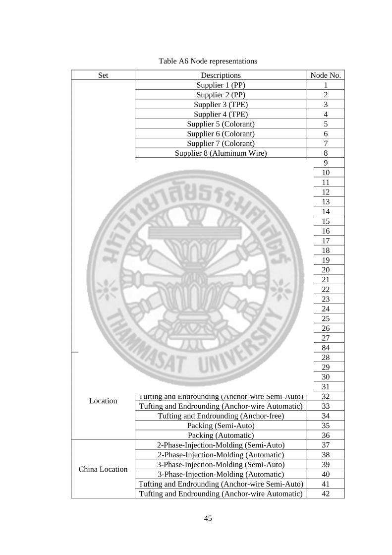
45

Table A6 Node representations

Set Descriptions Node No.

Suppliers

Supplier 1 (PP) 1 Supplier 2 (PP) 2

Supplier 3 (TPE) 3 Supplier 4 (TPE) 4

Supplier 5 (Colorant) 5 Supplier 6 (Colorant) 6 Supplier 7 (Colorant) 7

Supplier 8 (Aluminum Wire) 8 Supplier 9 (Aluminum Wire) 9

Supplier 10 (Brass Wire) 10 Supplier 11 (Brass Wire) 11 Supplier 12 (Filament) 12 Supplier 13 (Filament) 13 Supplier 14 (Filament) 14

Supplier 15 (PVC) 15 Supplier 16 (PVC) 16 Supplier 17 (PVC) 17 Supplier 18 (PVC) 18 Supplier 19 (PVC) 19

Supplier 20 (Shipper) 20 Supplier 21 (Shipper) 21 Supplier 22 (Shipper) 22 Supplier 23 (Shipper) 23

Supplier 24 (Backer Card) 24 Supplier 25 (Backer Card) 25 Supplier 26 (Backer Card) 26 Supplier 27 (Backer Card) 27

Supplier 28 (BR) 84

Vietnam Location

2-Phase-Injection-Molding (Semi-Auto) 28 2-Phase-Injection-Molding (Automatic) 29 3-Phase-Injection-Molding (Semi-Auto) 30 3-Phase-Injection-Molding (Automatic) 31

Tufting and Endrounding (Anchor-wire Semi-Auto) 32 Tufting and Endrounding (Anchor-wire Automatic) 33

Tufting and Endrounding (Anchor-free) 34 Packing (Semi-Auto) 35 Packing (Automatic) 36

China Location



46


India Location




Brazil Location




Customers

Australia 64 Russia 65 Turkey 66 Poland 67

Romania 68 Thailand 69

Philippines 70 Vietnam 71

China 72 India 73

Malaysia 74 Taiwan 75

Hong Kong 76 US 77

Canada 78 Mexico 79

Colombia 80 Brazil 81 GSS 82

East Africa 83

47

Table A7 Network arcs

From Node To Node Commodity Transportation Cost 1 28 {"PP"} 0.00012 2 28 {"PP"} 0.00023 3 28 {"TPE"} 0.00009 4 28 {"TPE"} 0.00009

84 28 {"BR"} 0.00051 5 28 {"Colorant"} 0.00001 6 28 {"Colorant"} 0.00009 7 28 {"Colorant"} 0.00012 1 29 {"PP"} 0.00012 2 29 {"PP"} 0.00023 3 29 {"TPE"} 0.00009 4 29 {"TPE"} 0.00009




84 37 {"BR"} 0.00043 5 37 {"Colorant"} 0.00009 6 37 {"Colorant"} 0.00001 7 37 {"Colorant"} 0.00011 1 38 {"PP"} 0.00011 2 38 {"PP"} 0.00020 3 38 {"TPE"} 0.00001

48

4 38 {"TPE"} 0.00001 84 38 {"BR"} 0.00043 5 38 {"Colorant"} 0.00009 6 38 {"Colorant"} 0.00001 7 38 {"Colorant"} 0.00011 1 39 {"PP"} 0.00011 2 39 {"PP"} 0.00020 3 39 {"TPE"} 0.00001 4 39 {"TPE"} 0.00001





84 48 {"BR"} 0.00050 5 48 {"Colorant"} 0.00012 6 48 {"Colorant"} 0.00011 7 48 {"Colorant"} 0.00001 1 49 {"PP"} 0.00001

49

2 49 {"PP"} 0.00012 3 49 {"TPE"} 0.00011 4 49 {"TPE"} 0.00011





84 58 {"BR"} 0.00027 5 58 {"Colorant"} 0.00066 6 58 {"Colorant"} 0.00061 7 58 {"Colorant"} 0.00054 8 32 {"Aluminum Wire"} 0.00009 9 32 {"Aluminum Wire"} 0.00009

10 32 {"Brass Wire"} 0.00035 11 32 {"Brass Wire"} 0.00033 12 32 {"Filament"} 0.00009 13 32 {"Filament"} 0.00009 14 32 {"Filament"} 0.00009

50

8 33 {"Aluminum Wire"} 0.00009 9 33 {"Aluminum Wire"} 0.00009

10 33 {"Brass Wire"} 0.00035 11 33 {"Brass Wire"} 0.00033 12 33 {"Filament"} 0.00009 13 33 {"Filament"} 0.00009 14 33 {"Filament"} 0.00009 8 34 {"Aluminum Wire"} 0.00009 9 34 {"Aluminum Wire"} 0.00009






10 51 {"Brass Wire"} 0.00027 11 51 {"Brass Wire"} 0.00024

51

12 51 {"Filament"} 0.00011 13 51 {"Filament"} 0.00011 14 51 {"Filament"} 0.00011 8 52 {"Aluminum Wire"} 0.00011 9 52 {"Aluminum Wire"} 0.00011




10 61 {"Brass Wire"} 0.00031 11 61 {"Brass Wire"} 0.00033 12 61 {"Filament"} 0.00061 13 61 {"Filament"} 0.00061 14 61 {"Filament"} 0.00061 15 35 {"PVC"} 0.00001 16 35 {"PVC"} 0.00006 17 35 {"PVC"} 0.00009 18 35 {"PVC"} 0.00066 19 35 {"PVC"} 0.00012 20 35 {"Shipper"} 0.00735 21 35 {"Shipper"} 0.09045 22 35 {"Shipper"} 0.11737 23 35 {"Shipper"} 0.65786 24 35 {"Backer Card"} 0.00735 25 35 {"Backer Card"} 0.09045 26 35 {"Backer Card"} 0.11737 27 35 {"Backer Card"} 0.65786 15 36 {"PVC"} 0.00001 16 36 {"PVC"} 0.00006

52

17 36 {"PVC"} 0.00009 18 36 {"PVC"} 0.00066 19 36 {"PVC"} 0.00012 20 36 {"Shipper"} 0.00735 21 36 {"Shipper"} 0.09045 22 36 {"Shipper"} 0.11737 23 36 {"Shipper"} 0.65786 24 36 {"Backer Card"} 0.00735 25 36 {"Backer Card"} 0.09045 26 36 {"Backer Card"} 0.11737 27 36 {"Backer Card"} 0.65786 15 44 {"PVC"} 0.00009 16 44 {"PVC"} 0.00005 17 44 {"PVC"} 0.00001 18 44 {"PVC"} 0.00061 19 44 {"PVC"} 0.00011 20 44 {"Shipper"} 0.09045 21 44 {"Shipper"} 0.01103 22 44 {"Shipper"} 0.10978 23 44 {"Shipper"} 0.61194 24 44 {"Backer Card"} 0.09045 25 44 {"Backer Card"} 0.01103 26 44 {"Backer Card"} 0.10978 27 44 {"Backer Card"} 0.61194 15 45 {"PVC"} 0.00009 16 45 {"PVC"} 0.00005 17 45 {"PVC"} 0.00001 18 45 {"PVC"} 0.00061 19 45 {"PVC"} 0.00011 20 45 {"Shipper"} 0.09045 21 45 {"Shipper"} 0.01103 22 45 {"Shipper"} 0.10978 23 45 {"Shipper"} 0.61194 24 45 {"Backer Card"} 0.09045 25 45 {"Backer Card"} 0.01103 26 45 {"Backer Card"} 0.10978 27 45 {"Backer Card"} 0.61194 15 53 {"PVC"} 0.00012 16 53 {"PVC"} 0.00015 17 53 {"PVC"} 0.00011 18 53 {"PVC"} 0.00054 19 53 {"PVC"} 0.00001 20 53 {"Shipper"} 0.11737 21 53 {"Shipper"} 0.10978 22 53 {"Shipper"} 0.00809 23 53 {"Shipper"} 0.54360

53

24 53 {"Backer Card"} 0.11737 25 53 {"Backer Card"} 0.10978 26 53 {"Backer Card"} 0.00809 27 53 {"Backer Card"} 0.54360 15 54 {"PVC"} 0.00012 16 54 {"PVC"} 0.00015 17 54 {"PVC"} 0.00011 18 54 {"PVC"} 0.00054 19 54 {"PVC"} 0.00001 20 54 {"Shipper"} 0.11737 21 54 {"Shipper"} 0.10978 22 54 {"Shipper"} 0.00809 23 54 {"Shipper"} 0.54360 24 54 {"Backer Card"} 0.11737 25 54 {"Backer Card"} 0.10978 26 54 {"Backer Card"} 0.00809 27 54 {"Backer Card"} 0.54360 15 62 {"PVC"} 0.00066 16 62 {"PVC"} 0.00065 17 62 {"PVC"} 0.00061 18 62 {"PVC"} 0.00001 19 62 {"PVC"} 0.00054 20 62 {"Shipper"} 0.65786 21 62 {"Shipper"} 0.61194 22 62 {"Shipper"} 0.54360 23 62 {"Shipper"} 0.00992 24 62 {"Backer Card"} 0.65786 25 62 {"Backer Card"} 0.61194 26 62 {"Backer Card"} 0.54360 27 62 {"Backer Card"} 0.00992 15 63 {"PVC"} 0.00066 16 63 {"PVC"} 0.00065 17 63 {"PVC"} 0.00061 18 63 {"PVC"} 0.00001 19 63 {"PVC"} 0.00054 20 63 {"Shipper"} 0.65786 21 63 {"Shipper"} 0.61194 22 63 {"Shipper"} 0.54360 23 63 {"Shipper"} 0.00992 24 63 {"Backer Card"} 0.65786 25 63 {"Backer Card"} 0.61194 26 63 {"Backer Card"} 0.54360 27 63 {"Backer Card"} 0.00992 35 64 {"SKU C","SKU I","SKU K"} 0.19033 35 65 {"SKU C","SKU I","SKU K"} 0.19438 35 66 {"SKU C","SKU I","SKU K"} 0.27863

54

35 67 {"SKU C","SKU I","SKU K"} 0.32093 35 68 {"SKU C","SKU I","SKU K"} 0.30820 35 69 {"SKU C","SKU I","SKU K"} 0.02973 35 70 {"SKU C","SKU I","SKU K"} 0.05927 35 71 {"SKU C","SKU I","SKU K"} 0.00735 35 72 {"SKU C","SKU I","SKU K"} 0.09045 35 73 {"SKU C","SKU I","SKU K"} 0.11737 35 74 {"SKU C","SKU I","SKU K"} 0.04764 35 75 {"SKU C","SKU I","SKU K"} 0.06816 35 76 {"SKU C","SKU I","SKU K"} 0.04064 35 77 {"SKU C","SKU I","SKU K"} 0.50764 35 78 {"SKU C","SKU I","SKU K"} 0.42577 35 79 {"SKU C","SKU I","SKU K"} 0.56044 35 80 {"SKU C","SKU I","SKU K"} 0.57087 35 81 {"SKU C","SKU I","SKU K"} 0.65786 35 82 {"SKU C","SKU I","SKU K"} 0.20782 35 83 {"SKU C","SKU I","SKU K"} 0.29041 36 64 {"SKU C","SKU I","SKU K"} 0.19033 36 65 {"SKU C","SKU I","SKU K"} 0.19438 36 66 {"SKU C","SKU I","SKU K"} 0.27863 36 67 {"SKU C","SKU I","SKU K"} 0.32093 36 68 {"SKU C","SKU I","SKU K"} 0.30820 36 69 {"SKU C","SKU I","SKU K"} 0.02973 36 70 {"SKU C","SKU I","SKU K"} 0.05927 36 71 {"SKU C","SKU I","SKU K"} 0.00735 36 72 {"SKU C","SKU I","SKU K"} 0.09045 36 73 {"SKU C","SKU I","SKU K"} 0.11737 36 74 {"SKU C","SKU I","SKU K"} 0.04764 36 75 {"SKU C","SKU I","SKU K"} 0.06816 36 76 {"SKU C","SKU I","SKU K"} 0.04064 36 77 {"SKU C","SKU I","SKU K"} 0.50764 36 78 {"SKU C","SKU I","SKU K"} 0.42577 36 79 {"SKU C","SKU I","SKU K"} 0.56044 36 80 {"SKU C","SKU I","SKU K"} 0.57087 36 81 {"SKU C","SKU I","SKU K"} 0.65786 36 82 {"SKU C","SKU I","SKU K"} 0.20782 36 83 {"SKU C","SKU I","SKU K"} 0.29041 44 64 {"SKU C","SKU I","SKU K"} 0.27499 44 65 {"SKU C","SKU I","SKU K"} 0.10502 44 66 {"SKU C","SKU I","SKU K"} 0.21890 44 67 {"SKU C","SKU I","SKU K"} 0.24430 44 68 {"SKU C","SKU I","SKU K"} 0.23827 44 69 {"SKU C","SKU I","SKU K"} 0.08262 44 70 {"SKU C","SKU I","SKU K"} 0.11848 44 71 {"SKU C","SKU I","SKU K"} 0.09045 44 72 {"SKU C","SKU I","SKU K"} 0.01103

55


56


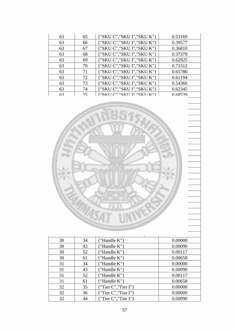
57

63 65 {"SKU C","SKU I","SKU K"} 0.53169 63 66 {"SKU C","SKU I","SKU K"} 0.39577 63 67 {"SKU C","SKU I","SKU K"} 0.36810 63 68 {"SKU C","SKU I","SKU K"} 0.37378 63 69 {"SKU C","SKU I","SKU K"} 0.62925 63 70 {"SKU C","SKU I","SKU K"} 0.71512 63 71 {"SKU C","SKU I","SKU K"} 0.65786 63 72 {"SKU C","SKU I","SKU K"} 0.61194 63 73 {"SKU C","SKU I","SKU K"} 0.54360 63 74 {"SKU C","SKU I","SKU K"} 0.62345 63 75 {"SKU C","SKU I","SKU K"} 0.68539 63 76 {"SKU C","SKU I","SKU K"} 0.67333 63 77 {"SKU C","SKU I","SKU K"} 0.26920 63 78 {"SKU C","SKU I","SKU K"} 0.34232 63 79 {"SKU C","SKU I","SKU K"} 0.23471 63 80 {"SKU C","SKU I","SKU K"} 0.11899 63 81 {"SKU C","SKU I","SKU K"} 0.00992 63 82 {"SKU C","SKU I","SKU K"} 0.45569 63 83 {"SKU C","SKU I","SKU K"} 0.36750 28 32 {"Handle C","Handle I"} 0.00000 28 33 {"Handle C","Handle I"} 0.00000 28 41 {"Handle C","Handle I"} 0.00090 28 42 {"Handle C","Handle I"} 0.00090 28 50 {"Handle C","Handle I"} 0.00117 28 51 {"Handle C","Handle I"} 0.00117 28 59 {"Handle C","Handle I"} 0.00658 28 60 {"Handle C","Handle I"} 0.00658 29 32 {"Handle C","Handle I"} 0.00000 29 33 {"Handle C","Handle I"} 0.00000 29 41 {"Handle C","Handle I"} 0.00090 29 42 {"Handle C","Handle I"} 0.00090 29 50 {"Handle C","Handle I"} 0.00117 29 51 {"Handle C","Handle I"} 0.00117 29 59 {"Handle C","Handle I"} 0.00658 29 60 {"Handle C","Handle I"} 0.00658 30 34 {"Handle K"} 0.00000 30 43 {"Handle K"} 0.00090 30 52 {"Handle K"} 0.00117 30 61 {"Handle K"} 0.00658 31 34 {"Handle K"} 0.00000 31 43 {"Handle K"} 0.00090 31 52 {"Handle K"} 0.00117 31 61 {"Handle K"} 0.00658 32 35 {"Tier C","Tier I"} 0.00000 32 36 {"Tier C","Tier I"} 0.00000 32 44 {"Tier C","Tier I"} 0.00090

58

32 45 {"Tier C","Tier I"} 0.00090 32 53 {"Tier C","Tier I"} 0.00117 32 54 {"Tier C","Tier I"} 0.00117 32 62 {"Tier C","Tier I"} 0.00658 32 63 {"Tier C","Tier I"} 0.00658 33 35 {"Tier C","Tier I"} 0.00000 33 36 {"Tier C","Tier I"} 0.00000 33 44 {"Tier C","Tier I"} 0.00090 33 45 {"Tier C","Tier I"} 0.00090 33 53 {"Tier C","Tier I"} 0.00117 33 54 {"Tier C","Tier I"} 0.00117 33 62 {"Tier C","Tier I"} 0.00658 33 63 {"Tier C","Tier I"} 0.00658 34 35 {"Tier K"} 0.00000 34 36 {"Tier K"} 0.00000 34 44 {"Tier K"} 0.00090 34 45 {"Tier K"} 0.00090 34 53 {"Tier K"} 0.00117 34 54 {"Tier K"} 0.00117 34 62 {"Tier K"} 0.00658 34 63 {"Tier K"} 0.00658 37 32 {"Handle C","Handle I"} 0.00090 37 33 {"Handle C","Handle I"} 0.00090 37 41 {"Handle C","Handle I"} 0.00000 37 42 {"Handle C","Handle I"} 0.00000 37 50 {"Handle C","Handle I"} 0.00110 37 51 {"Handle C","Handle I"} 0.00110 37 59 {"Handle C","Handle I"} 0.00612 37 60 {"Handle C","Handle I"} 0.00612 38 32 {"Handle C","Handle I"} 0.00090 38 33 {"Handle C","Handle I"} 0.00090 38 41 {"Handle C","Handle I"} 0.00000 38 42 {"Handle C","Handle I"} 0.00000 38 50 {"Handle C","Handle I"} 0.00110 38 51 {"Handle C","Handle I"} 0.00110 38 59 {"Handle C","Handle I"} 0.00612 38 60 {"Handle C","Handle I"} 0.00612 39 34 {"Handle K"} 0.00090 39 43 {"Handle K"} 0.00000 39 52 {"Handle K"} 0.00110 39 61 {"Handle K"} 0.00612 40 34 {"Handle K"} 0.00090 40 43 {"Handle K"} 0.00000 40 52 {"Handle K"} 0.00110 40 61 {"Handle K"} 0.00612 41 35 {"Tier C","Tier I"} 0.00090

59

41 36 {"Tier C","Tier I"} 0.00090 41 44 {"Tier C","Tier I"} 0.00000 41 45 {"Tier C","Tier I"} 0.00000 41 53 {"Tier C","Tier I"} 0.00110 41 54 {"Tier C","Tier I"} 0.00110 41 62 {"Tier C","Tier I"} 0.00612 41 63 {"Tier C","Tier I"} 0.00612 42 35 {"Tier C","Tier I"} 0.00090 42 36 {"Tier C","Tier I"} 0.00090 42 44 {"Tier C","Tier I"} 0.00000 42 45 {"Tier C","Tier I"} 0.00000 42 53 {"Tier C","Tier I"} 0.00110 42 54 {"Tier C","Tier I"} 0.00110 42 62 {"Tier C","Tier I"} 0.00612 42 63 {"Tier C","Tier I"} 0.00612 43 35 {"Tier K"} 0.00090 43 36 {"Tier K"} 0.00090 43 44 {"Tier K"} 0.00000 43 45 {"Tier K"} 0.00000 43 53 {"Tier K"} 0.00110 43 54 {"Tier K"} 0.00110 43 62 {"Tier K"} 0.00612 43 63 {"Tier K"} 0.00612 46 32 {"Handle C","Handle I"} 0.00117 46 33 {"Handle C","Handle I"} 0.00117 46 41 {"Handle C","Handle I"} 0.00110 46 42 {"Handle C","Handle I"} 0.00110 46 50 {"Handle C","Handle I"} 0.00000 46 51 {"Handle C","Handle I"} 0.00000 46 59 {"Handle C","Handle I"} 0.00544 46 60 {"Handle C","Handle I"} 0.00544 47 32 {"Handle C","Handle I"} 0.00117 47 33 {"Handle C","Handle I"} 0.00117 47 41 {"Handle C","Handle I"} 0.00110 47 42 {"Handle C","Handle I"} 0.00110 47 50 {"Handle C","Handle I"} 0.00000 47 51 {"Handle C","Handle I"} 0.00000 47 59 {"Handle C","Handle I"} 0.00544 47 60 {"Handle C","Handle I"} 0.00544 48 34 {"Handle K"} 0.00117 48 43 {"Handle K"} 0.00110 48 52 {"Handle K"} 0.00000 48 61 {"Handle K"} 0.00544 49 34 {"Handle K"} 0.00117 49 43 {"Handle K"} 0.00110 49 52 {"Handle K"} 0.00000

60

49 61 {"Handle K"} 0.00544 50 35 {"Tier C","Tier I"} 0.00117 50 36 {"Tier C","Tier I"} 0.00117 50 44 {"Tier C","Tier I"} 0.00110 50 45 {"Tier C","Tier I"} 0.00110 50 53 {"Tier C","Tier I"} 0.00000 50 54 {"Tier C","Tier I"} 0.00000 50 62 {"Tier C","Tier I"} 0.00544 50 63 {"Tier C","Tier I"} 0.00544 51 35 {"Tier C","Tier I"} 0.00117 51 36 {"Tier C","Tier I"} 0.00117 51 44 {"Tier C","Tier I"} 0.00110 51 45 {"Tier C","Tier I"} 0.00110 51 53 {"Tier C","Tier I"} 0.00000 51 54 {"Tier C","Tier I"} 0.00000 51 62 {"Tier C","Tier I"} 0.00544 51 63 {"Tier C","Tier I"} 0.00544 52 35 {"Tier K"} 0.00117 52 36 {"Tier K"} 0.00117 52 44 {"Tier K"} 0.00110 52 45 {"Tier K"} 0.00110 52 53 {"Tier K"} 0.00000 52 54 {"Tier K"} 0.00000 52 62 {"Tier K"} 0.00544 52 63 {"Tier K"} 0.00544 55 32 {"Handle C","Handle I"} 0.00658 55 33 {"Handle C","Handle I"} 0.00658 55 41 {"Handle C","Handle I"} 0.00612 55 42 {"Handle C","Handle I"} 0.00612 55 50 {"Handle C","Handle I"} 0.00544 55 51 {"Handle C","Handle I"} 0.00544 55 59 {"Handle C","Handle I"} 0.00000 55 60 {"Handle C","Handle I"} 0.00000 56 32 {"Handle C","Handle I"} 0.00658 56 33 {"Handle C","Handle I"} 0.00658 56 41 {"Handle C","Handle I"} 0.00612 56 42 {"Handle C","Handle I"} 0.00612 56 50 {"Handle C","Handle I"} 0.00544 56 51 {"Handle C","Handle I"} 0.00544 56 59 {"Handle C","Handle I"} 0.00000 56 60 {"Handle C","Handle I"} 0.00000 57 34 {"Handle K"} 0.00658 57 43 {"Handle K"} 0.00612 57 52 {"Handle K"} 0.00544 57 61 {"Handle K"} 0.00000 58 34 {"Handle K"} 0.00658

61

58 43 {"Handle K"} 0.00612 58 52 {"Handle K"} 0.00544 58 61 {"Handle K"} 0.00000 59 35 {"Tier C","Tier I"} 0.00658 59 36 {"Tier C","Tier I"} 0.00658 59 44 {"Tier C","Tier I"} 0.00612 59 45 {"Tier C","Tier I"} 0.00612 59 53 {"Tier C","Tier I"} 0.00544 59 54 {"Tier C","Tier I"} 0.00544 59 62 {"Tier C","Tier I"} 0.00000 59 63 {"Tier C","Tier I"} 0.00000 60 35 {"Tier C","Tier I"} 0.00658 60 36 {"Tier C","Tier I"} 0.00658 60 44 {"Tier C","Tier I"} 0.00612 60 45 {"Tier C","Tier I"} 0.00612 60 53 {"Tier C","Tier I"} 0.00544 60 54 {"Tier C","Tier I"} 0.00544 60 62 {"Tier C","Tier I"} 0.00000 60 63 {"Tier C","Tier I"} 0.00000 61 35 {"Tier K"} 0.00658 61 36 {"Tier K"} 0.00658 61 44 {"Tier K"} 0.00612 61 45 {"Tier K"} 0.00612 61 53 {"Tier K"} 0.00544 61 54 {"Tier K"} 0.00544 61 62 {"Tier K"} 0.00000 61 63 {"Tier K"} 0.00000

62

Appendix B

OPL Model

********************************************* * OPL 12.6.0.0 Model * Author: Administrator * Creation Date: Aug 25, 2015 at 10:43:40 AM *********************************************/ {int} V =...; //set of nodes in the network {int} S =...; //set of nodes representing suppliers {int} C =...; //set of nodes representing customers {int} O =...; //set of capacity options {string} States ={"pessimistic","most likely","optimistic"}; //BOM Structure tuple BOM { string Master_Item; string Sub_Item; float Conversion; } {BOM} BOM_Data=...; //Material tuple Material{ string Item_Name; string Category; } {Material} Material_Data=...; {string} K =...; //set of components (or commodites) {string} K_Dummy=...; //set of dummy components {string} F =...; //set of finished goods tuple Process{ int Node; {string} Output; // Components or Product produced by the Process } {Process} P =...; //information about requirement of each process; tuple Edge{ int fromnode; //Origin Node int tonode; //Destination Node {string} commodity; //Required Components float transport_cost; //Transportation cost }; {Edge} Edges=...; //Arc connecting nodes over the network

63

tuple Location{ {int}Associated_Nodes; }; {Location} L=...; float Ultilization_Target=...; float Production_Limit_Ratio=...; float Unit_Sourcing_Cost[S][K]=...;//Sourcing cost of component k using supplier s float Unit_Production_Cost [States][O][V diff (S union C)][K union F]=...;//Production cost of component k using a capacity level at a location float Unit_Shortage_Cost[F]=...; //Cost for each unsatisfied demand int Demand[States][C][F]=...; //Demand at each customer location int Open[States][L]=...; // Cost of Opening a location int Setup[States][ V diff (S union C)][O]=...; // Cost of installing a kind of capacity in a location int Cap[V diff (S union C)][O]=...; // Capacity for each option in a location int Sup[S][K]=...; // Supply capacity of suppliers //Decision Variables dvar boolean Y[L]; //Location Decision dvar boolean Z[V diff (S union C)][O]; //Option Decision dvar int+ X[Edges][K_Dummy union F][O]; //Flow Quantity dvar int+ Shortage[States][C][F]; //Shortage Demand dvar float+ alpha; //Cost Expression //Opening Cost term in most likely situation dexpr float Opening_Cost_M = sum (event in States:event=="most likely",l in L)Y[l]*Open[event][l]; //Opening Cost term in optimistic situation dexpr float Opening_Cost_O = sum (event in States:event=="optimistic",l in L)Y[l]*Open[event][l]; //Opening Cost term in pessimistic situation

64

dexpr float Opening_Cost_P = sum (event in States:event=="pessimistic",l in L)Y[l]*Open[event][l]; //Setup Cost term in most likely situation dexpr float Setup_Cost_M = sum (event in States:event=="most likely",i in V diff (S union C), o in O)Z[i][o]*Setup[event][i][o]; //Setup Cost term in optimistic situation dexpr float Setup_Cost_O = sum (event in States:event=="optimistic",i in V diff (S union C), o in O)Z[i][o]*Setup[event][i][o]; //Setup Cost term in pessimistic situation dexpr float Setup_Cost_P = sum (event in States:event=="pessimistic",i in V diff (S union C), o in O)Z[i][o]*Setup[event][i][o]; dexpr float Transportation_Cost = sum (e in Edges,k in K_Dummy union F,o in O)X[e][k][o]*e.transport_cost; dexpr float Procurement_Cost = sum (s in S, e in Edges: e.fromnode==s,k_dummy in K_Dummy,m in Material_Data:m.Item_Name==k_dummy, k in e.commodity:k==m.Category, o in O)X[e][k_dummy][o]*Unit_Sourcing_Cost[e.fromnode][k]; //Production Cost term in most likely situation dexpr float Production_Cost_M = sum (event in States:event=="most likely",i in V diff (S union C), e in Edges: e.fromnode==i, k in e.commodity,o in O)X[e][k][o]*Unit_Production_Cost[event][o][e.fromnode][k]; //Production Cost term in optimistic situation dexpr float Production_Cost_O = sum (event in States:event=="optimistic",i in V diff (S union C), e in Edges: e.fromnode==i, k in e.commodity,o in O)X[e][k][o]*Unit_Production_Cost[event][o][e.fromnode][k]; //Production Cost term in pessimistic situation dexpr float Production_Cost_P = sum (event in States:event=="pessimistic",i in V diff (S union C), e in Edges: e.fromnode==i, k in e.commodity,o in O)X[e][k][o]*Unit_Production_Cost[event][o][e.fromnode][k]; //Shortage Cost term in pessimistic situation dexpr float Shortage_Cost_P=sum(event in States:event=="pessimistic",i in C,k in F)Shortage[event][i][k]*Unit_Shortage_Cost[k]; //Shortage Cost term in most likely situation dexpr float Shortage_Cost_M=sum(event in States:event=="most likely",i in C,k in F)Shortage[event][i][k]*Unit_Shortage_Cost[k]; //Opening Cost term in optimistic situation dexpr float Shortage_Cost_O=sum(event in States:event=="optimistic",i in C,k in F)Shortage[event][i][k]*Unit_Shortage_Cost[k]; //Total Cost in pessimistic situation dexpr float z_p = Opening_Cost_P+Setup_Cost_P+Transportation_Cost+Procurement_Cost+Production_Cost_P+Shortage_Cost_P; //Total Cost in most likely situation

65

dexpr float z_m = Opening_Cost_M+Setup_Cost_M+Transportation_Cost+Procurement_Cost+Production_Cost_M+Shortage_Cost_M; //Total Cost in optimistic situation dexpr float z_o = Opening_Cost_O+Setup_Cost_O+Transportation_Cost+Procurement_Cost+Production_Cost_O+Shortage_Cost_O; //Objective Function //minimize Opening_Cost+Setup_Cost+Transportation_Cost+Procurement_Cost+Production_Cost+Shortage_Cost_P; //******************************* // Epsilon Approach //******************************* //minimize z_o; // Iteration 1 //minimize z_m; // Iteration 2 //Replication 1 minimize z_o; // Iteration 1 ‐ relax pessimistic by 5% //Replication 2 //minimize z_m; // Iteration 1 ‐ relax pessimistic by 5% //minimize z_o; // Iteration 2 ‐ relax pessimistic by 5% //******************************* // //******************************* //Constraints subject to{ //******************************* // Epsilon Approach //******************************* //z_o<= 48043527; //Iternation 1 ‐ relax pessimistic by 5% //z_p<= 65392421*1.05; //z_o<= 48043527; //Iternation 2 ‐ relax pessimistic by 5% z_p<= 65392421*1.05; z_m<= 50799666; //******************************* // //*******************************

66

//Supply ctSupply: forall (i in S, k in K) sum (e in Edges: e.fromnode==i, k1 in K_Dummy, m in Material_Data:m.Item_Name==k1, c in e.commodity:c==m.Category&&c==k,o in O:o==1)X[e][k1][o]<=Sup[i][k]; forall (i in S, k in K) sum (e in Edges: e.fromnode==i, k1 in K_Dummy, m in Material_Data:m.Item_Name==k1, c in e.commodity:c==m.Category&&c==k,o in O:o!=1)X[e][k1][o]<=0; //Demand ctDemand: forall (event in States, i in C, k in F) sum (e in Edges: e.tonode==i, c in e.commodity:c==k, o in O)X[e][k][o]>=Demand[event][i][k]‐Shortage[event][i][k]; forall (event in States, i in C, k in F) Shortage[event][i][k]<=Demand[event][i][k]; //Balance ctBalance: forall (h in V diff (S union C)) forall (p in P: p.Node==h, comp in p.Output,b in BOM_Data: b.Master_Item==comp) sum (e1 in Edges:e1.tonode==h, c1 in K_Dummy: c1==b.Sub_Item, m in Material_Data:m.Item_Name==c1, c in e1.commodity:c==m.Category, o in O)X[e1][c1][o]/b.Conversion== sum (e2 in Edges:e2.fromnode==h,c2 in e2.commodity:c2==comp,o in O)X[e2][c2][o]; //Node constraint ctUpper_Capacity_Limit: forall (h in V diff (S union C), o in O) sum (e in Edges:e.fromnode==h,c in e.commodity)X[e][c][o]<=Z[h][o]*Cap[h][o]; //Location Constraint ctLocation: forall (l in L, l1 in l.Associated_Nodes, i in V diff(S union C):i==l1, o in O)Z[i][o]<=Y[l]; //Capacity Selection ctCapacity: forall (i in V diff (S union C)) sum (o in O)Z[i][o]<=1; }

optimal design of supply chain network: a case study in

Documents