optimal demand response - the resnick sustainability ...resnick.caltech.edu/docs/sg_low.pdf ·...

Optimal Demand Response

Libin Jiang Steven Low

Computing + Math Sciences Electrical Engineering

Caltech

Oct 2011

Outline

Caltech smart grid research

Optimal demand response

Global trends

1 Exploding renewables   Driven by sustainability   Enabled by policy and investment

2 Migration to distributed arch   2-3x generation efficiency   Relief demand on grid capacity

Source: Renewable Energy Global Status Report, 2010 Source: M. Jacobson, 2011

Wind power over land (exc. Antartica) 70 – 170 TW

Solar power over land 340 TW

Worldwide

energy demand: 16 TW

electricity demand: 2.2 TW

wind capacity (2009): 159 GW

grid-tied PV capacity (2009): 21 GW

High Levels of Wind and Solar PV Will Present an Operating Challenge!

Source: Rosa Yang, EPRI

Key challenge: uncertainty mgt

Large-scale active network of DER

DER: PVs, wind turbines, batteries, EVs, DR loads

Large-scale active network of DER

DER: PVs, wind turbines, batteries, EVs, DR loads

Millions of active endpoints introducing rapid large !

random fluctuations !in supply and demand!

Control challenges

Need to close the loop   Real-time feedback control   Driven by uncertainty of renewables

Scalability   Orders of magnitude more endpoints that can

generate, compute, communicate, actuate   Driven by new power electronics, distributed arch

Engineering + economics   Need interdisciplinary holistic approach   Power flow determined by markets as well as physics

Current control

local

global

slow fast

relay system

SCADA EMS

•  centralized •  state estimation •  contingency analysis •  optimal power flow •  simulation •  human in loop •  decentralized

•  mechanical

mainly centralized, open-loop preventive, slow timescale

Our approach

local

global

relay system

SCADA EMS

endpoint based scalable control

•  local algorithms •  global perspective

scalable, decentralized, real-time feedback, sec-min timescale

slow fast

Our approach

local

global

relay system

SCADA EMS

endpoint based scalable control

•  local algorithms •  global perspective

We have technologies to monitor/control 1,000x faster not the fundamental theories and algorithms

slow fast

Our approach Endpoint based control

  Self-manage through local sensing, communication, control

  Real-time, scalable, closed-loop, distributed, robust

Local algorithms with global perspective   Simple algorithms   Globally coordinated

Control and optimization framework   Systematic algorithm design   Clarify ideas, explore structures, suggest direction

Ambitious, comprehensive, multidisciplinary Start with concrete relevant component projects

Our approach: benefits Scalable, adaptive to uncertainty

  By design

Robust understandable global behavior   Global behavior of interacting local algorithms can be

cryptic and fragile if not designed thoughtfully

Improved reliability & efficiency

Real-time price Flat Price, Scenario 1 Flat Price, Scenario 2

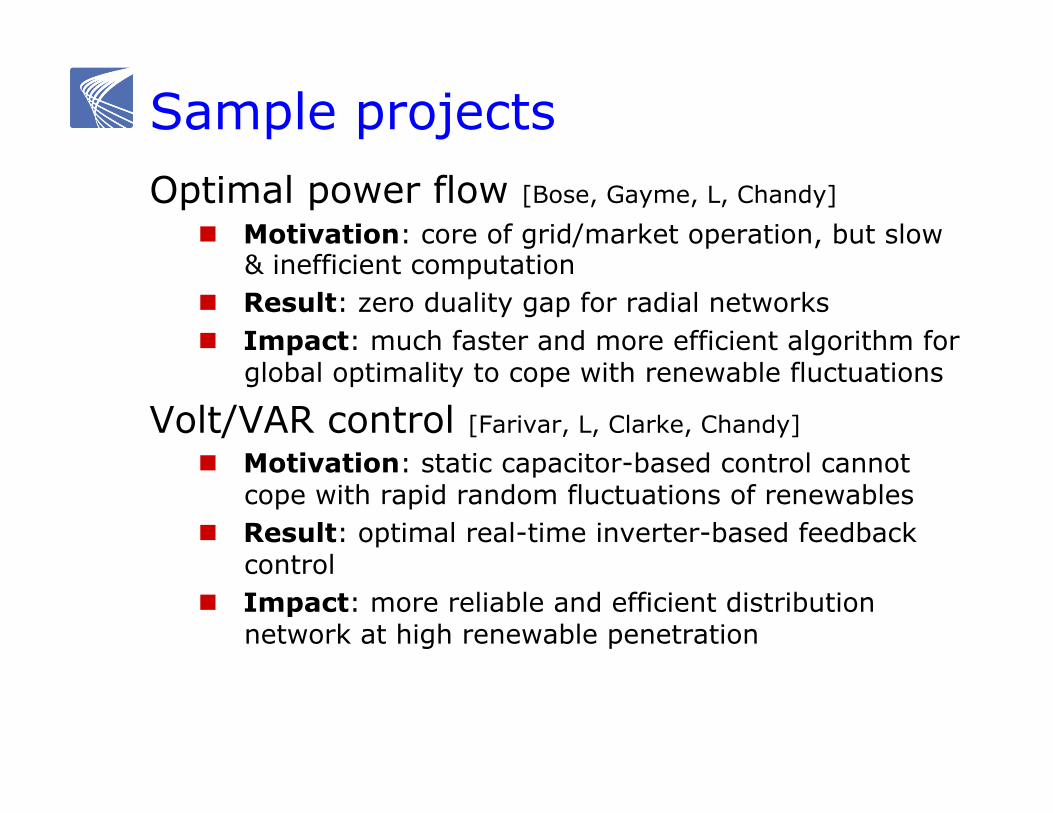
Sample projects Optimal power flow [Bose, Gayme, L, Chandy]

  Motivation: core of grid/market operation, but slow & inefficient computation

  Result: zero duality gap for radial networks   Impact: much faster and more efficient algorithm for

global optimality to cope with renewable fluctuations

Volt/VAR control [Farivar, L, Clarke, Chandy]   Motivation: static capacitor-based control cannot

cope with rapid random fluctuations of renewables   Result: optimal real-time inverter-based feedback

control   Impact: more reliable and efficient distribution

network at high renewable penetration

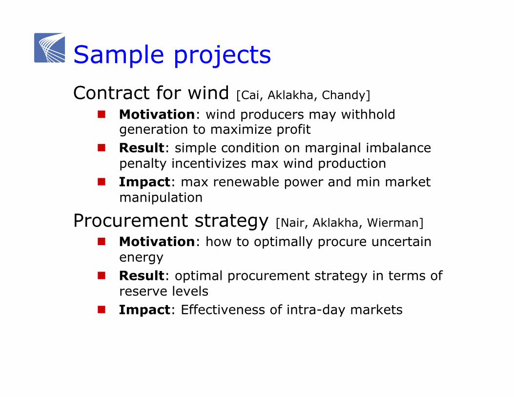
Sample projects Contract for wind [Cai, Aklakha, Chandy]

  Motivation: wind producers may withhold generation to maximize profit

  Result: simple condition on marginal imbalance penalty incentivizes max wind production

  Impact: max renewable power and min market manipulation

Procurement strategy [Nair, Aklakha, Wierman]   Motivation: how to optimally procure uncertain

energy   Result: optimal procurement strategy in terms of

reserve levels

  Impact: Effectiveness of intra-day markets

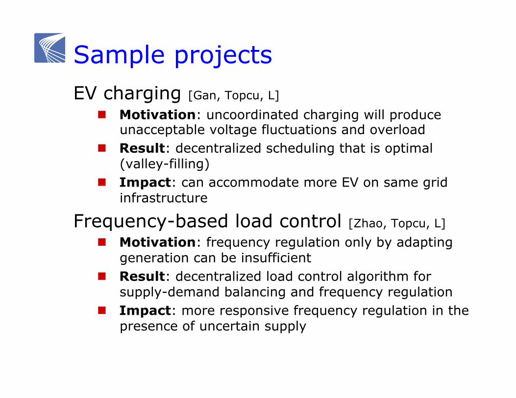
Sample projects EV charging [Gan, Topcu, L]

  Motivation: uncoordinated charging will produce unacceptable voltage fluctuations and overload

  Result: decentralized scheduling that is optimal (valley-filling)

  Impact: can accommodate more EV on same grid infrastructure

Frequency-based load control [Zhao, Topcu, L]   Motivation: frequency regulation only by adapting

generation can be insufficient   Result: decentralized load control algorithm for

supply-demand balancing and frequency regulation

  Impact: more responsive frequency regulation in the presence of uncertain supply

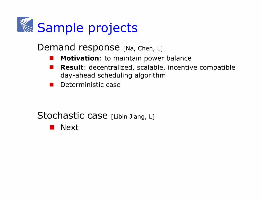
Sample projects Demand response [Na, Chen, L]

  Motivation: to maintain power balance   Result: decentralized, scalable, incentive compatible

day-ahead scheduling algorithm   Deterministic case

Stochastic case [Libin Jiang, L]

  Next

Outline

Caltech smart grid research

Optimal demand response   Model   Results

Features to capture Wholesale markets

  Day ahead, real-time balancing Renewable generation

  Non-dispatchable

Demand response   Real-time control (through pricing)

day ahead balancing renewable

utility

users

utility

users

Model: user Each user has 1 appliance (wlog)

  Operates appliance with probability

  Attains utility ui(xi(t)) when consumes xi(t)

Demand at t:

!i =1 wp " i (t) 0 wp 1!" i (t)"#$

D(t) := !i xi (t)i!

xi (t) ! xi (t) ! xi (t) xi (t)t" # Xi

P d (t), cd P d (t)( ), co !x(t)( )

Model: LSE (load serving entity)

Power procurement   Renewable power:

  Random variable, realized in real-time

  Day-ahead power:

  Control, decided a day ahead

  Real-time balancing power:

 

•  Use as much renewable as possible •  Optimally provision day-ahead power •  Buy sufficient real-time power to balance demand

capacity

energy

Simplifying assumption

 No network constraints

Questions Day-ahead decision

  How much power should LSE buy from day-ahead market?

Real-time decision (at t-)   How much should users consume, given

realization of wind power and ?

How to compute these decisions distributively? How does closed-loop system behave ?

t- t – 24hrs

available info:

decision:

Our approach Real-time (at t-)

  Given and realizations of , choose optimal to max social welfare, through DR

Day-ahead   Choose optimal that maximizes expected

optimal social welfare

xi* = xi

* Pd;Pr,!i( )

t-

Pr,!i

t – 24hrs

available info:

decision:

Pd


Model

Results   Without time correlation: distributed alg   With time correlation: distributed alg   Impact of uncertainty

No time correlation: T=1 Each user has 1 appliance (wlog)



Demand at t:

!i =1 wp " i (t) 0 wp 1!" i (t)"#$

D(t) := !i xi (t)i!


Welfare function Supply cost

Welfare function (random)

c Pd, x( ) = cd P d( )+ co !(x)( )0Pd + cb !(x)"P d( )+

!(x) := !i xii" #P r

W Pd, x( ) = !iuii! (xi )" c Pd, x( )

excess demand

user utility supply cost



!(x) := !i xii" #P r excess demand

!(x)cd Pd( ) cd !(x)( )0Pd cb !(x)"Pd( )+




!(x) := !i xii" #P r

W Pd, x( ) = !iuii! (xi )" c Pd, x( )

excess demand

user utility supply cost

Optimal operation


Optimal real-time demand response

Optimal day-ahead procurement

W Pd, x( ) = !iuii! (xi )" c Pd, x( )

x* Pd( ) := arg maxxW Pd, x( ) given realization

of P r ,!i

Pd* := arg max

Pd EW Pd, x

* Pd( )( )

maxPd

E maxxW Pd, x( )Overall problem:

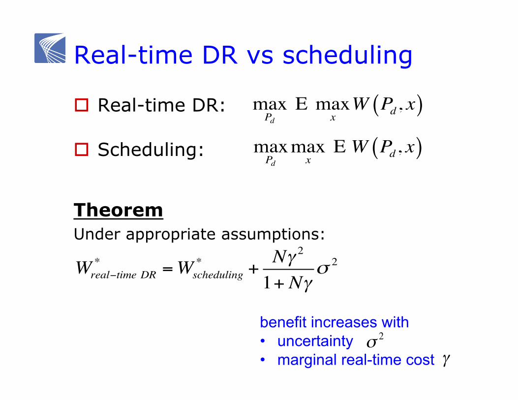
Real-time DR vs scheduling

maxPd

E maxxW Pd, x( )  Real-time DR:

  Scheduling: maxPd

maxx

E W Pd, x( )

Theorem Under appropriate assumptions:

Wreal!time DR* =Wscheduling

* +N! 2

1+ N!" 2

benefit increases with •  uncertainty •  marginal real-time cost

! 2

!

Algorithm 1 (real-time DR)

Active user i computes   Optimal consumption

LSE computes   Real-time “price”   Optimal day-ahead energy to use   Optimal real-time balancing energy

xi*

µb*

yo*

yb*

maxPd

E maxxW Pd, x( )

real-time DR

Active user i : xik+1 = xi

k +! ui ' xik( )!µb

k( )( )xi

xi

inc if marginal utility > real-time price

LSE : µbk+1 = µb

k +! ! xk( )" yok " ybk( )( )+

inc if total demand > total supply


•  Decentralized •  Iterative computation at t-

Theorem: Algorithm 1 Socially optimal

  Converges to welfare-maximizing DR   Real-time price aligns marginal cost of supply

with individual marginal utility

Incentive compatible   max i’s surplus given price

x* = x* Pd( )


µb*xi

*

µb* = c ' Pd,! x*( )( ) = ui ' xi*( )

More precisely: µb* !"xc Pd,# x*( )( )

pricing = marginal cost


µb*

= co ' ! x*( )( ) if 0<! x*( ) < Pd= cb ' ! x*( )"Pd( ) if Pd<! x*( )# co ' ! x*( )( ),cb ' ! x*( )"Pd( )$%

&' if ! x*( ) = Pd

(

)

**

+

**

Theorem: Algorithm 1

Marginal costs, optimal day-ahead and balancing power consumed:


cb' yb

*( ) = co' yo*( )+µo*

µo* =

!W!Pd

Pd*( )

if Pd* > 0

Algorithm 2 (day-ahead procurement)

Optimal day-ahead procurement maxPd

EW Pd, x* Pd( )( )

Pdm+1 = Pd

m +! m µom ! cd ' Pd

m( )( )( )+

LSE:

calculated from Monte Carlo simulation of Alg 1

(stochastic approximation)


Optimal day-ahead procurement maxPd

EW Pd, x* Pd( )( )

LSE:

µom =

!W!Pd

Pdm( )

µbm = µo

m + co' yo

m( )

Given !m,Prm :

Pdm+1 = Pd

m +! m µom ! cd ' Pd

m( )( )( )+

Theorem

Algorithm 2 converges a.s. to optimal for appropriate stepsize

Pd*


! k


Model

Results   Without time correlation: distributed alg   With time correlation: distributed alg   Impact of uncertainty

General T case Each user has 1 appliance (wlog)



Demand at t:

!i =1 wp " i (t) 0 wp 1!" i (t)"#$

D(t) := !i xi (t)i!


Coupling across time Need state

Time correlation

  Example: EV charging   Time-correlating constraint:

  Day-ahead decision and real-time decisions

  (1+T)-period dynamic programming

Day-ahead

available info:

decision:

t- t = 1,2,…, T

Remaining demand

Algorithm 3 (T>1)

  Main idea   Solve deterministic problem in each step using

conditional expectation of Pr (distributed)   Apply decision at current step

  One day ahead, decide Pd* by solving

  At time t-, decide x*(t) by solving

Theorem: performance   Algorithm 3 is optimal in special cases

 

Algorithm 3 (T>1)

J * ! J A3 !1

T ! t +1

t=1

T

! ! 2 (t)

Impact of renewable on welfare

Pr (t;a,b) := a !µ(t)+ b !V (t)

mean

Renewable power:

zero-mean RV

Optimal welfare of (1+T)-period DP

W * a,b( )

Impact of renewable on welfare

Theorem   Cost increases in var of

  increases in a, decreases in b   increases in s (plant size)

W * a,b( )Pr

Pr (t;a,b) := a !µ(t)+ b !V (t)

W * s, s( )

optimal demand response - the resnick sustainability ...resnick.caltech.edu/docs/sg_low.pdf ·...

Documents