optimal cross training in call centers with uncertain...

Optimal Cross Training in Call Centers with Uncertain

Arrivals and Global Service Level Agreements Working Paper Draft

Thomas R. Robbins • D. J. Medeiros • Terry P. Harrison

Pennsylvania State University, University Park, PA We consider agent cross-training in project oriented call centers where arrival rates are

uncertain and the call center is subject to a global service level constraint. This paper is

motivated by work with a provider of outsourced technical support services in which most

projects include an inbound tier one help desk subject to a monthly service level agreement

(SLA). Support services are highly specialized and a significant training investment is

required, an investment that is not transferable to other projects. We investigate the option of

cross training a subset of agents so that they may serve calls from two separate projects, a

process we refer to as partial pooling. Our paper seeks to quantity the benefits of partial

pooling and characterize the conditions under which pooling is most beneficial. We then

determine the optimal number of agents to cross train given the training investment and

incremental wage paid to cross skilled agents. We find that cross training a modest portion of

the staff yields significant benefits.

Optimal Cross Training Working Paper – August 3, 2007

1 Introduction

Call centers are a critical component of the worldwide services infrastructure and are often tightly

linked with other large scale services. Many outsourcing arrangements, for example, contain

some level of call center support, often delivered from offshore locations. A call center is a

facility designed to support the delivery of some interactive service via telephone

communications; typically an office space with multiple workstations manned by agents who

place and receive calls (Gans, Koole et al. 2003). Call centers are a large and growing

component of the U.S. and world economy, by 2008 the United States will employ an estimated

2.1 million call center agents (Aksin, Armony et al. 2007). Large scale call centers are

technically and managerially sophisticated operations and have been the subject of substantial

academic research. Call center applications include telemarketing, customer service, help desk

support, and emergency dispatch.

Staffing is a critical issue in call center management as direct labor costs often account for 60-

80% of the total operating budget of a call center (Aksin, Armony et al. 2007). This paper

addresses the scheduling problem in a call center with highly variable and uncertain arrival rates.

The work is directly related to a research project with a provider of outsourced technical support

delivered via globally distributed call centers. The company provides both tier 1 (help desk) and

tier 2 (desk-side) support. The bulk of their business, and the focus of this research, is on the

inbound call center operation. This operation involves providing help desk support to large

corporate and government entities. While the scope of services varies from account to account,

many accounts are 24 x 7 support and virtually all accounts are subject to some form of Service

Level Agreement (SLA). There are multiple types of SLA, but the most common specifies a

minimum level of the Telephone Service Factor (TSF). A TSF SLA specifies the proportion of

calls that must be answered within a specified time. For example, an 80/120 SLA specifies that

80% of calls must be answered within 120 seconds. A very important point is that the service

level applies to an extended period, typically a month. The SLA does not define requirements for

a day or an hour. So the desk is often staffed so that at some times the service level is

underachieved, sometimes overachieved, and is on target for the entire month.


The key challenge involved with staffing this call center is meeting a fixed SLA with a variable

and uncertain arrival rate pattern. The number of calls presented in any ½ hour period is highly

variable with multiple sources of uncertainty. In the following figure we see daily call volume

for a typical project shown over a 3 month period.

Calls Offered Daily

0

100

200

300

400

500

600

700

800

900

4/1 4/6 4/11 4/16 4/21 4/26 5/1 5/6 5/11 5/16 5/21 5/26 5/31 6/5 6/10 6/15 6/20 6/25 6/30

Calls_Offered-Daily 7 per. Mov. Avg. (Calls_Offered-Daily) Figure 1-1 Sample Daily Arrival Pattern

This graph shows strong “seasonal” variation over the course of a week. Monday’s tend to be the

highest volume days with volumes dropping off over the course of the week. Call volume on

Saturday is a small fraction of the weekday volume, and this particular desk is closed on Sundays.

The graph also reveals significant stochastic variability. Tuesdays are, for example, often higher

volume then Wednesdays but this is not always the case. During the weeks of 4/26 and 5/16 we

see larger volumes on Wednesday then Tuesday. We also see the issue of unanticipated spikes in

demand, often referred to as significant events. This is an extremely common event in support

desk operations. A downed server, for example, will generate a large call volume. While some

contracts provide SLA relief in the case of significant events, in general the desk must meet SLA

even when significant events occur. The large volume of calls during a significant event not only

result in poor performance, but also represents a large portion of total calls received making it

more difficult to achieve the overall SLA.

In addition to day of week seasonality these call centers also experience very significant time of

day seasonality. Volume tends to dip down around the lunch break, but a second peak occurs in


the afternoon; though the afternoon peak is typically lower volume then the morning peak. While

this basic arrival pattern exists on most business days, there is significant stochastic variability in

the call pattern from day to day. The following graph shows call volume over an eight week

period for a particular project. The inner region represents the minimum volume presented in

each period, while the overall envelope is the maximum volume presented in each period. The

outer region then represents the variability over this eight week period.

Figure 1-2 Range of Call Volume

This particular desk operates 24x7 and we see that the volume during the overnight hours is quite

low. Volume ramps up sharply in the morning with a major surge of calls between 7 and 11 AM.

Volume tends to dip down around the lunch break, but a second peak occurs in the afternoon,;

though the afternoon peak is typically lower volume then the morning peak. The staffing

challenge in this call center is to find a minimal cost staffing plan that achieves a global service

level target with a high probability. The schedule must obviously be locked in before arrival rate

uncertainty is revealed.

In Section 2 we briefly review the relevant literature. Section 3 presents presents the basic call

center configuration examined in the rest of the paper. In section 4 we examine optimal cross

training in steady state conditions. In section 5 we examine the use of partial pooling in a more

Range of Call Volume 8 week sample

0

10

20

30

40

50

60

70

80

M T W R F Sa Su

Calls per half hour

MaxMin


realistic setting, with an uncertain time varying arrival process. We use a combination of

optimization and simulation based analysis to find a near optimal schedule of standard and pooled

agents. Section 6 provides extension and future directions for research.

2 Literature

Call centers have been the focus of significant academic research. A detailed of the call center

oriented literature is provided in (Gans, Koole et al. 2003). More recent work is summarized in

(Aksin, Armony et al. 2007). Empirical analysis of call center data is provided in (Brown, Gans

et al. 2005).

The issue of cross training in call centers is summarized in (Aksin, Karaesmen et al. 2007). The

cross training literature for call centers builds on the extensive cross training literature in the

context of manufacturing and supply chain operations (Graves and Tomlin 2003; Hopp, Tekin et

al. 2004; Hopp and Van Oyen 2004). Cross training is relevant in call centers where agents are

segregated by skill set and skills based routing is employed. Issues related to staffing and routing

in multi-skill call centers are summarized in (Koole and Pot 2005). Routing issues in the context

of call center outsourcing are discussed in (Gans and Zhou 2007). Models that address

scheduling in multi skill call centers are provided in (Avramidis, Chan et al. 2007; Avramidis,

Gendreau et al. 2007; Cezik and L'Ecuyer 2007). (Iravani, Kolfal et al. 2007) develop a heuristic

to evaluate the effectiveness of different cross training options.

A paper very similar in concept to ours is (Wallace and Whitt 2005). In the W&W model there

are 6 call types and every agent is trained to handle a fixed number of those types. The authors

use a simulation based optimization model to find the ideal cross training level. The paper’s key

insight is that a low level of cross training provides “most” of the benefit. Specifically, they find

that training every agent in 2 skills provides the bulk of the benefit, while additional training has a

relatively low payoff. In the W&W model all agents are cross trained with the same number of

skills. (Robbins, Medeiros et al. 2007) examine the impact of partial pooling in steady state

queuing systems. They examine the impact of cross training a small number of agents to handle

two different call types and find that cross training a small portion of the agents provides most of

the benefit. Both of these models ignore the incremental costs associated with cross training and

fail to find the optimal cross training level.


3 Pooling Model

3.1 Overview In this section we introduce our model of partial pooling. We first introduce some basic

terminology and notation we use throughout the paper. We assume that in the baseline case the

call center is segregated by project and each project acts a separate Erlang-A queuing system.

Each project i receives calls that arrive with a potentially time varying rate ( )i tλ . Associated

with each call is a average talk time denoted as 1 iµ . We also assume that callers have

exponentially distributed patience with mean 1 iθ . The patience parameter represents the time a

caller is willing to wait on hold. Each caller will abandon the queue (hang up) if not server by

their patience parameter. The details of the Erlang-A model are provided in (Mandelbaum and

Zeltyn 2004). Methods for approximating Erlang A results are described in (Garnett,

Mandelbaum et al. 2002). An assessment of the Erlang-A models to parameter sensitivity is

provided in (Whitt 2006)

3.2 Routing We now examine the issue of cross training super agents to see how this impacts service levels.

We examine the case of cross training between two projects and assume that the skills based

routing system is configured as follows:

Figure 3-1 Basic Routing Structure


We have two call types, one for each project, and three agent pools. Pool 1 has skill 1 and can

service call type 1. Similarly pool 2 services call types 2. Pool 3 is cross trained and can service

calls from either queue.

We implement a very simple routing model. An incoming call is routed to a base agent if one is

available. Only in the case where all base agents are busy is the call routed to a super agent. As

long as super agents remain available all calls will be serviced immediately and no abandonment

will take place. If no qualified agents are available the call is queued to be served by the next

available agent. When base agents become available they take the longest waiting caller from

their respective queue. If no calls are waiting they become idle. When a super agent becomes

available they take the call from the largest queue.

3.3 System Costs and Objective Our staffing objective for this call center is to satisfy a service level objective for each call type

with a high probability while minimizing overall staffing cost. Because call volume is stochastic

and subject to random shocks it is not practical to meet the service level target with certainty. We

therefore chose to implement the service level target as a soft constraint; applying a penalty cost

to a realized service level below the target.

The primary cost of operation of the call center is staffing. We assume that cross trained agents

are more expensive than base agents. This is a result both of the additional cost of training plus

the wage premium that must be paid to these higher skilled agents.

Our system has three staffing levels denoted as , 1, 2,3ix i = , each of which is paid a wage iw .

Similarly we have 2 call type with service level goals jg , realized service levels jS , and penalty

rates jr , for 1, 2j = . The total cost of operating the system is given by

1 1 2 2 3 2 1 1 1 2 2 2( ) ( )TC w x w x w x r g S r g S+ += + + + − + − (3.1)

Our objective is to select the staffing vector that minimizes the expected cost of operating the

system.


4 Optimal Cross Training in Steady State

4.1 Overview In this section we examine the impact of partial pooling in a steady state environment; that is an

environment where arrivals follow on a homogeneous Poisson process. The impact of partial

pooling under steady state conditions is examined in detail in (Robbins, Medeiros et al. 2007).

They show that a moderate level of pooling yields significant benefit but the benefits of pooling

are rapidly declining. This is consistent with Property 5 in (Aksin, Karaesmen et al. 2007);

“Well designed limited resource flexibility is almost as good as full resource flexibility in terms of

performance”.

(Robbins, Medeiros et al. 2007) show that the service level increases as agents are crossed

trained, but that the incremental benefit drops off quickly. This suggests, assuming cross training

is costly, that cross training more than a moderate proportion of the work force is sub optimal. In

this section we examine this issue more rigorously and attempt to find the optimal level of cross

training. To do this we relax the assumption of a fixed resource pool. The optimization problem

then becomes selecting the staffing vector that defines the number of agents in each pool so as to

minimize the expected cost of operation.

4.2 A Simulation Based Optimization Method We use a simulation based local search algorithm to find the optimal cross training pattern for any

given parameter setting. The local search algorithm is guided by a variable neighborhood search

(VNS) metaheuristic. VNS is a metaheuristic that makes systematic changes in the neighborhood

being searched as the search progresses (Hansen and Mladenovic 2001; Hansen and Mladenovic

2005). When using VNS a common approach is to define a set of nested neighborhoods, such

that

1 2( ) ( ) ... ( )MaxkN x N x N x x X⊂ ⊂ ⊂ ∀ ∈ (4.1)

The general structure of the VNS is then as follow:

Initialization


Select the set of neighborhood structures ,kN for max1,...,k k=

Construct an initial incumbent solution, Ix , using some heuristic procedure.

Select a confidence level α for the selection of a new incumbent solution

Search: repeat the following until Stop=True

Set 1k =

Find minkn candidate solutions, Cx that are neighbors of Ix

Simulate the system with each candidate and compare the results to the incumbent

using a pairwise T Test.

If any Cx is superior to Ix at the α level then set *I Cx x= , where *

Cx is the best

candidate solution

Else, set minki n= , set found = false, and repeat until (

maxki n= or found=True)

Find a new candidate ikx

Simulate the system with each candidate and compare the results using a

pairwise T Test.

If ikx is superior to Ix at the α level then set

iI kx x= and found = True

If a no new incumbent was found in neighborhood k then

set 1k k= +

maxk k> then Stop = True

Figure 4-1 General VNS Search Algorithm

This algorithm searches the neighborhood of the current incumbent evaluating at least

minkn points. If no statistically improving solution is found it continues to search until either an

improving solution is found or a total of maxkn points have been evaluated. Each time an

improving solution is found the search restarts with the new incumbent. If no new incumbent is

found the search continues in the next largest neighborhood. The search process continues until

no improving solution is found in the largest neighborhood structure.


Two important parameters for this search process are minkn and

maxkn , the lower and upper bounds

on the number of neighbors to evaluate before moving to the next neighborhood. If the

neighborhood is defined narrowly these parameters are both set equal to the total number of

neighbors and the neighborhood is searched exhaustively. In larger neighborhoods an exhaustive

search is not practical and solutions are selected at random. In this case minkn is the minimum

number of neighbors to evaluate. Setting this parameter to one implements a first improving local

search.

4.3 Optimal Cross Training with Known Arrival Rates In the case of steady state arrivals with known rates, two different neighborhoods are defined.

1N is the neighborhood of all 1-changes; that is the set of all feasible solutions ix such that one

element differs from cx by either 1 or -1. For any incumbent there are up to 6 solutions in this

neighborhood. 1N is the neighborhood of all 2-changes; that is the set of all feasible solutions

ix such that exactly two element differ from cx by either 1 or -1. For any incumbent there are up

to 12 solutions in this neighborhood.

In this experiment we seek to determine the optimal staffing vector for a steady state process with

known arrival rates. We are interested in determining how the staffing vector is impacted by the

relative arrival rates as well as management decisions related to the desired quality of service.

Specifically we create a two level full factorial design in four factors as shown below.


A B C D Variable Factor Definitions - +1 - - - - A Arrival Rate 2 100 2002 + - - - B Service Level Requirement 70/120 85/603 - + - - C Penalty Rate/hr 5 15 4 + + - - D Pooled wage differential 10% 40%5 - - + -6 + - + -7 - + + - Constant Factors8 + + + - Arrival Rate 1 1009 - - - + Talk Time (min) 12

10 + - - + Mean time to Abandon (sec) 35011 - + - +12 + + - +13 - - + +14 + - + +15 - + + +16 + + + +

Table 4-1 Cross Training with Steady State Known Arrivals – Experimental Design

We ran this experiment using a version of the VNS algorithm outlined in Figure 4-1. For each

configuration we simulated two days of operations and performed 10 replications. The search

moved to a new solution if the pair wise comparison showed an improvement at the 80%

confidence level.

The results of this optimization are shown in the following table.

A B C D N1 N2 N3 % PooledAverage

TSF Average

Total CostAverage Penalty

1 - - - - 17 17 2 5.6% 70.2% 17,759 3832 + - - - 17 31 4 7.7% 69.1% 25,693 5413 - + - - 21 21 3 6.7% 86.2% 21,872 1284 + + - - 21 39 4 6.3% 85.1% 31,226 3145 - - + - 17 17 3 8.1% 73.9% 17,904 06 + - + - 17 32 4 7.5% 72.3% 25,808 1767 - + + - 21 21 3 6.7% 86.2% 22,154 4108 + + + - 21 40 4 6.2% 93.6% 32,496 1,1049 - - - + 17 17 2 5.6% 70.1% 18,120 456

10 + - - + 17 32 3 5.8% 69.2% 26,082 54611 - + - + 21 21 3 6.7% 86.2% 22,297 12112 + + - + 21 40 3 4.7% 85.0% 31,718 42213 - - + + 17 17 3 8.1% 73.7% 18,336 014 + - + + 17 32 4 7.5% 72.1% 26,338 13015 - + + + 21 21 3 6.7% 86.2% 22,584 40816 + + + + 21 40 4 6.2% 87.2% 32,025 57

Staffing VectorFactors Metrics


Table 4-2 Cross Training with Steady State Known Arrivals – Experimental Results

This data shows that in all cases examined partial pooling is beneficial and the optimal solution

always includes some level of cross training. In this analysis the optimal number of cross trained

agents covers a relatively narrow range. The optimal solution always has at least two, but no more

than four cross trained agents. Cross trained agents represent between 4.7% and 8.1% of the total

labor pool. The algorithm also sets staffing levels such that the service level is very close to the

target level. However, because this is fundamentally a discrete optimization problem, the service

level can not be set to an arbitrary level and it is sometime optimal to allow a small expected

penalty cost.

4.4 Optimal Cross Training with Uncertain Loads In the previous section we calculated the optimal staffing vector when arrival rates are known and

constant. We found that in all cases we examined the optimal staffing choice called for some

level of cross trained resources, even though those resources are more costly than base level

resources. In this section we relax the assumption that arrival rates are known and examine how

this impacts the optimal staffing vector.

We conduct an experiment similar to the experiment outlined in table 4-1 with the exception that

the arrivals rates are normally distributed around the original set points with a coefficient of

variation of .1.



TSF Average

Total Average Penalty

1 - - - - 17 17 3 8.1% 77.7% 17,904 02 + - - - 17 32 4 7.5% 75.5% 25,632 03 - + - - 21 21 3 6.7% 89.5% 21,744 04 + + - - 21 40 4 6.2% 90.0% 31,392 05 - - + - 17 17 5 12.8% 84.4% 18,960 06 + - + - 17 32 6 10.9% 80.8% 26,688 07 - + + - 21 20 6 12.8% 94.1% 22,848 08 + + + - 21 39 7 10.4% 93.6% 32,496 09 - - - + 17 17 3 8.1% 77.7% 18,336 0

10 + - - + 17 33 3 5.7% 75.4% 26,016 011 - + - + 21 21 3 6.7% 89.5% 22,176 012 + + - + 21 40 3 4.7% 88.0% 31,308 1213 - - + + 17 17 4 10.5% 83.6% 19,488 48014 + - + + 17 33 5 9.1% 80.8% 27,360 015 - + + + 21 21 5 10.6% 93.8% 23,520 016 + + + + 21 40 6 9.0% 93.5% 33,312 0

Staffing VectorFactors Metrics

Table 4-3 Cross Training with Steady State Uncertain Arrivals – Experimental Results

In the uncertain arrival case the level of cross training is in general increased, total costs in

general increase, and the service level penalty is effectively eliminated. The difference between

these two experiments is summarized in the following table:


TSF Average

Total CostAverage Penalty

1 - - - - 0 0 1 2.6% 7.5% 144.6 -383.42 + - - - 0 1 0 -0.1% 6.4% -60.7 -540.73 - + - - 0 0 0 0.0% 3.3% -127.8 -127.84 + + - - 0 1 0 -0.1% 4.9% 166.1 -313.95 - - + - 0 0 2 4.7% 10.5% 1,056.0 0.06 + - + - 0 0 2 3.4% 8.4% 879.5 -176.57 - + + - 0 -1 3 6.1% 7.9% 693.8 -410.28 + + + - 0 -1 3 4.3% 0.0% 0.0 -1,104.09 - - - + 0 0 1 2.6% 7.7% 216.4 -455.6

10 + - - + 0 1 0 -0.1% 6.2% -66.3 -546.311 - + - + 0 0 0 0.0% 3.3% -120.8 -120.812 + + - + 0 0 0 0.0% 3.0% -410.5 -410.513 - - + + 0 0 1 2.4% 9.9% 1,152.0 480.014 + - + + 0 1 1 1.5% 8.7% 1,021.9 -130.115 - + + + 0 0 2 4.0% 7.6% 936.0 -408.016 + + + + 0 0 2 2.8% 6.3% 1,286.7 -57.3

Average 0 0.1 1.1 2.1% 6.4% 422.9 -294.1

Factors Staffing Vector Metrics

Table 4-4 Comparison of Known and Uncertain Arrival Experiments

There are a few key observations from this analysis:


• Uncertainty increases cost – the total cost of operation increased by an average of $422.

The cost of service delivery increased significantly in the high penalty rate cases, where

service level attainment is important.

• Pooling is more effective in uncertain situations – more pooling was added in the

uncertain arrival cases, and the service level penalty was effectively eliminated in the

uncertain case. With uncertain arrivals the probability of a capacity mismatch is higher,

and therefore the benefits of dynamic capacity reallocation are higher.

5 Optimal Cross Training with Time Varying Arrivals

5.1 Overview In the previous section we analyzed the impact of pooling on steady state stationary behavior. As

described in Section 1, real call centers often face arrival rates that vary significantly across the

course of the day. Because arrival rates vary considerably call centers must change the staff

level throughout the course of the day. In the call center projects we analyzed staffing varies

from two agents over night, to as many as 70 agents during peak hours. On a 24 hour schedule

the call center may have shifts starting during any 30 minute period. But because the vast

majority of agents are scheduled to full time shifts, the call center can not vary the staff as quickly

as demand varies. The call center is therefore subject to periods of tight capacity and excess

capacity in any given day.

Conceptually, the objective of this optimization problem is to find the minimal cost staffing plan

that meets the service level requirement with the appropriate level of confidence. However, the

nonstationary scheduling introduces a few additional considerations. In particular we require

staffing to meet a minimum level at all times (typically 2 agents) and a level of staffing such that

at expected volumes we achieve some minimal service level (typically 50%). While it is possible

to modify the neighborhood structure to enforce these hard constraints, a more straightforward

search mechanism results if soften these constraints and add them as penalty terms to the

objective function.


5.2 The Optimization-Simulation Approach In this approach we generate a preliminary schedule for each project independently using an

optimization program and then run a local search via simulation to optimize the overall project.

To develop an initial feasible solution we run an optimization program for each project

individually. We utilize the stochastic scheduling algorithm described in (Robbins 2007a;

Robbins 2007b) but in this instance the model is configured to generate a schedule at a lower TSF

and with a minimum staffing level of one instead of two agents. This procedure creates a staff

plan that is slightly understaffed. The objective is to create an initial plan where selective cross

training can yield rapid improvement.

To identify additional candidate solutions we implement a VNS as described in figure 4-1.

However, in this case the neighborhood structure is considerably more complex. We define a

nested neighborhood structure with five individual neighborhoods.

Let J be the set of schedules to which an agent may be assigned and denote as jx the number of

agents assigned to schedule j . A staff plan is a vector of jx values. A staff plan is feasible if

every jx is non-negative and integral valued. Assume that any complicating constraints, such as

minimum staffing levels, have been moved into the objective function as a penalty term. Denote

the set of feasible staff plans as X . Furthermore, define the sets iA J⊆ as the active schedules,

for resource pool i; that is the schedules to which at least one resource has been assigned and let

1 2 3A A A A= ∪ ∪ be the set of active schedules across pools.

Now, for some arbitrary x X∈ , define a series of nested neighborhood structures such that

1 2( ) ( ) ... ( )MaxkN x N x N x x X⊂ ⊂ ⊂ ∀ ∈ (4.2)

We define the following neighborhoods


• 1( )N x : Active 1 Change: the set of all staff plans where an active assignment is updated

by and additive offset, { }1,1iδ ∈ − .

• 2 ( )N x : Active 2 Change: pick any two feasible schedules in iA and independently

update each by { }1,0,1iδ ∈ − .

• 3( )N x : Feasible 1 Change: the set of all staff plans where a feasible assignment is

updated by { }1,1iδ ∈ − .

• 4 ( )N x : Feasible 2 Change: pick any two feasible schedules in J and independently


• 5 ( )N x : Feasible 3 Change: pick any three feasible schedules in J and independently


I each neighborhood a new schedules is selected randomly and a large number of alternative

schedules are evaluated at each iteration of the algorithm. While a pure random search will likely

find improving solutions if enough permutations are evaluated I have found that using certain

heuristic methods in each neighborhood improves the rate of convergence. In this modified

approach each time a new neighbor is required the algorithm picks either a heuristic or a pure

random permutation.

The following table summarizes the heuristics utilized in each neighborhood:

Neighborhood Heuristics

1( )N x : Active 1 Change - Pool Support: select an active schedule in Pool 1 or Pool 2 and staff an agent to the same schedule in the cross trained pool.

2 ( )N x : Active 2 Change - Cross Train: select an active schedule in Pool 1 or Pool 2 and change the agent’s designation to a cross trained agent.

- Untrain: select a staffed schedule in pool three and change the designation to either 1 or 2.

3( )N x : Feasible 1 Change - Add Max Cover: find the set of feasible schedules that covers the most short-staffed periods and schedule an agent to one of those schedules.


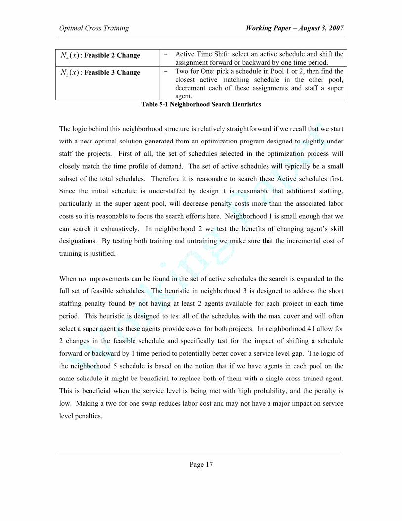
4 ( )N x : Feasible 2 Change - Active Time Shift: select an active schedule and shift the assignment forward or backward by one time period.

5 ( )N x : Feasible 3 Change - Two for One: pick a schedule in Pool 1 or 2, then find the closest active matching schedule in the other pool, decrement each of these assignments and staff a super agent.

Table 5-1 Neighborhood Search Heuristics

The logic behind this neighborhood structure is relatively straightforward if we recall that we start

with a near optimal solution generated from an optimization program designed to slightly under

staff the projects. First of all, the set of schedules selected in the optimization process will

closely match the time profile of demand. The set of active schedules will typically be a small

subset of the total schedules. Therefore it is reasonable to search these Active schedules first.

Since the initial schedule is understaffed by design it is reasonable that additional staffing,

particularly in the super agent pool, will decrease penalty costs more than the associated labor

costs so it is reasonable to focus the search efforts here. Neighborhood 1 is small enough that we

can search it exhaustively. In neighborhood 2 we test the benefits of changing agent’s skill

designations. By testing both training and untraining we make sure that the incremental cost of

training is justified.

When no improvements can be found in the set of active schedules the search is expanded to the

full set of feasible schedules. The heuristic in neighborhood 3 is designed to address the short

staffing penalty found by not having at least 2 agents available for each project in each time

period. This heuristic is designed to test all of the schedules with the max cover and will often

select a super agent as these agents provide cover for both projects. In neighborhood 4 I allow for

2 changes in the feasible schedule and specifically test for the impact of shifting a schedule

forward or backward by 1 time period to potentially better cover a service level gap. The logic of

the neighborhood 5 schedule is based on the notion that if we have agents in each pool on the

same schedule it might be beneficial to replace both of them with a single cross trained agent.

This is beneficial when the service level is being met with high probability, and the penalty is

low. Making a two for one swap reduces labor cost and may not have a major impact on service

level penalties.


In practice the largest number of improving solutions were found in neighborhood 1. Improving

solutions were found in every neighborhood, though not for every optimization. In a typical

optimization process improvements are found in three to four neighborhoods, though in some

cases all neighborhoods generated improvements. The number of solutions tested in each

iteration clearly varies based on where an improvement is found. By design most improvements

are found in the first neighborhood. In my experiment I required that at least 20 candidates were

tested before the best was selected. The max number varies with the number of active schedules,

as neighborhood 1 is searched exhaustively. In a typical scenario bout 300 candidate solutions

were tested in the final iteration of the algorithm, the iteration which found no improvements.

The total number of iterations until termination is also random, and depends on the number of

feasible schedules. The total number of iterations tended to vary between 15 and 25. All in all

this implies that an optimization effort will evaluate somewhere in the range of 500 to 1,500

different schedule combinations.

In terms of the selection of the metaheuristic, there are a very large number of algorithms

available including genetic algorithms, simulated annealing, and Tabu search as well as other

approaches such as gradient based search or response surface methods. Because the problem is

discrete I decided not to pursue gradient or response surface methods as these algorithms are

better suited to smooth response functions. Our choice of metaheuristic was driven by the

combinatorial nature of the problem. Technically the feasible set for the problem is unlimited.

Assume we place a practical limit of η as the total number of agents assigned to any schedule, the

number of feasible staff plans is 3 ηΝ where Ν is the number of feasible schedules for the

scheduling option. (see Table 4-10). The least flexible option (A) has 336 feasible schedules. If

we set η as 10 then there are approximately 3010 feasible schedules. For option F the number

expands to more than 4010 . We sought some algorithm that allowed other search heuristic (such

as those in Table 10-10) to be embedded into the overall algorithm. We rejected genertic

algorithms because there was no obvious way to implement a crossover mechanism that would

yield high quality solutions. In addition a population based approach increases the number of

solutions to be tested, and the simulation process makes evaluation relatively expensive. The

selection process is also more difficult when trying to select the best solution for a population vs.


a sequential pairwise comparison. Tabu Search is a viable approach and could in fact be added to

the current algorithm to prevent repeated evaluation of the same solution which clearly happens

in this algorithm. Simulated Annealing is another alternative to facilitate the breakout from local

optimum which is accomplished via expanded neighborhoods in this algorithm.

5.3 Project Level Comparisons

5.3.1 Overview

In this section we analyze the impact of partial pooling under real world situations. We attempt

to find optimal plans for cross training agents based on the arrival and talk time characteristics of

several actual outsourcing projects. Details of these projects are provided in (Robbins 2007b).

Project J is a corporate help desk for a large industrial company averaging about 750 calls a day

where the volatility of call volume is relatively low. Project S is a help desk that provides support

to employees of a large national retail chain. Call volume on this desk is about 2,000 calls a day.

Because this desk supports users in retail stores, as opposed to corporate offices, the daily

seasonality of call volumes is quite different from Project S. This company is making major

changes in its IT infrastructure and as such call volume is very volatile and difficult to forecast.

Project O is a help desk that provides support to corporate and retail site users of another retail

chain. This is a small desk with about 500 calls a day, where call volume is fairly volatile and

shocks are relatively common.

5.3.2 Pooled Optimization – Project J and S

In this section we test the impact of pooling Projects J and S. Recall that Project J is a corporate

project with relatively stable arrival patterns. Project S is a retail project with somewhat volatile

arrival patterns. Since one project is corporate and one is retail these projects have different

seasonality patterns. The busy period for project S extends later into the day, and the project has

busier weekends. Project S also has less of a lunchtime lull in call volume than Project J.

The following table summarizes the results of the pooled optimization effort:


Sched Set

Labor Cost

Expected Outcome TSF 1 TSF2

% Agents Pooled Labor Outcome TSF 1 TSF2

Labor Savings

Total Savings

% Savings

A 41,600 44,504 78.3% 83.5% 13.0% 41,356 42,560 83.2% 83.4% 244 1,944 4.4%B 40,400 44,504 78.1% 84.7% 15.3% 40,769 41,873 84.4% 83.6% -369 2,631 5.9%C 40,320 44,504 78.9% 85.0% 16.1% 40,424 41,171 83.0% 84.0% -104 3,333 7.5%D 40,120 44,504 79.4% 84.4% 17.0% 40,732 41,537 83.0% 84.3% -612 2,968 6.7%E 40,000 44,504 78.9% 85.3% 18.7% 40,197 41,664 81.4% 83.4% -197 2,840 6.4%

Individual Optimization Pooled Optimization Comparison

Table 5-2 Pooled Optimization – Projects J-S

The data shows that even with a 25% premium for pooled agents, pooling reduces the overall cost

of operation. Cost savings vary from 4.4% to 7.5% depending on the scheduling set option. In

each case the number of labor hours drawn from the cross trained pool is less than 20%. As was

the case in the steady state analysis, pooling a relatively small percentage of the agents provides

the optimal results. Note that Project J, the smaller project, sees an improvement in service level

in each case while the service level for Project S remains constant or declines slightly.

Intuitively, in the single pool case Project S must carry safety capacity to hedge against costly

spikes, which is evident by the average service level cushion or 3%-5%. In the pooled case spare

capacity can be allocated to Project J as necessary and each project has an average service level

just above the targeted level. Further insight can be gleaned from the graphical views of the

resulting staff plan. In the following figure we plot the staffing plan for schedule set C.

Pooled Staffing Plan Project J-S Schedule Set C

0

10

20

30

40

50

60

70

80

Pool 3Pool 2Pool 1

Figure 5-1 Pooled Staffing Plan


Pool 3 Staffing Plan - Project J-S Schedule Set C

0

2

4

6

8

10

12

1 12 23 34 45 56 67 78 89 100 111 122 133 144 155 166 177 188 199 210 221 232 243 254 265 276 287 298 309 320 331 Figure 5-2 Cross Trained Agent Staffing Plan

Cross trained agents are scheduled throughout the week but are most heavily deployed during the

busy periods.

5.3.3 Pooled Optimization Projects J-O

Similar results are found for the pairing of Project J and Project O as summarized below.

Sched Set

Labor Cost



Labor Savings

Total Savings

% Savings

A 23,200 24,606 78.3% 79.9% 14.3% 23,228 23,938 80.8% 81.2% -28 668 2.7%B 22,800 24,606 78.1% 78.5% 14.5% 22,834 23,547 81.7% 81.4% -34 1,060 4.3%C 22,800 24,606 78.9% 78.3% 21.2% 23,115 23,504 81.8% 82.3% -315 1,102 4.5%D 22,540 24,606 79.4% 79.7% 19.0% 23,143 23,758 80.7% 82.8% -603 848 3.4%E 22,460 24,606 78.9% 79.1% 18.8% 22,698 23,550 80.8% 81.5% -238 1,056 4.3%


Table 5-3 Pooled Optimization – Projects J-O

In this case the savings are slightly less, in the range of 2.7% - 4.3% and the proportion of agents

cost trained is slightly higher. In each case labor costs are increased slightly resulting in a higher

level of confidence that the service level goal will be achieved. The average service level of each

project improves in each case. Recalling that these projects are of approximately the same size

the benefits are roughly equally distributed. The average service level for each project moves up

from just below the target to just above the target. Intuitively, since the incremental capacity can

be allocated to either project as needed, the cost of incremental labor is offset by the reduction in

penalty costs.


5.3.4 Pooled Optimization Projects S-O

In this final pairing I examine a pooling of Project S and Project O, both of which have retail

oriented seasonality patterns. The results are summarized below:

Sched Set

Labor Cost



Labor Savings

Total Savings

% Savings

A 41,600 44,387 83.5% 79.9% 10.1% 40,654 42,349 82.4% 80.4% 946 2,038 4.6%B 40,800 44,387 84.7% 78.5% 13.7% 39,370 41,523 81.2% 80.6% 1,430 2,864 6.5%C 40,400 44,387 85.0% 78.3% 15.4% 40,034 41,966 82.8% 80.3% 366 2,421 5.5%D 40,540 44,387 84.4% 79.7% 14.5% 39,768 42,103 82.8% 79.8% 772 2,284 5.1%E 40,620 44,387 85.3% 79.1% 13.7% 40,273 42,188 82.5% 80.7% 347 2,199 5.0%


Table 5-4 Pooled Optimization – Projects S-O

As in the previous case pooling reduces cost of operation for these projects around 5% by pooling

10%-15% of agents. But unlike the two previous cases, this situation reduces total cost by

reducing labor. The intuition is that each of these projects is relatively volatile and must carry

significant spare capacity to hedge against uncertainty. By pooling, project spare capacity can be

shared and the total amount of spare capacity is reduced.

5.3.5 The Impact of Cross Training Wage Differential

The analysis shows that cross training a portion of the workforce can reduce costs even if cross

training resources is expensive. In the analysis so far we have assumed that cross training creates

a 25% cost premium. In this section we examine the impact of varying the wage differential.

For this experiment we test the same project and schedule pairs tested above, but allow the wage

differential to vary. I maintain the base agent wage at $10.00 per hour, but we test super agent

wage rates of $11.25, $12.00, and $13.75. Overall we find that cross training is a viable tactic

over this range of costs. The expected savings is naturally declining in the wage differential as is

the proportion of agents cross trained – although the proportion of agents cross trained is less

sensitive to the wage differential than one might expect. The results are summarized in the

following table


PairingSched

SetExpected Outcome

% Agents Pooled

% Savings

% Agents Pooled

% Savings

% Agents Pooled

% Savings

J-S A 44,504 15.3% 7.1% 13.0% 4.4% 14.3% 3.9%B 43,529 17.3% 5.7% 15.3% 3.8% 13.3% 3.7%C 43,780 15.9% 6.9% 16.1% 6.0% 15.1% 4.0%D 43,120 19.0% 5.4% 17.0% 3.7% 16.4% 2.6%E 43,240 19.4% 5.5% 18.7% 3.6% 17.4% 0.9%

J-O A 24,606 14.3% 4.1% 14.3% 2.7% 10.7% 0.9%B 24,643 19.6% 5.5% 14.5% 4.4% 16.1% 1.5%C 24,597 22.9% 5.8% 21.2% 4.4% 15.4% 2.5%D 24,396 28.3% 5.4% 19.0% 2.6% 14.9% 0.9%E 24,513 20.1% 6.3% 18.8% 3.9% 18.3% 0.6%

S-O A 44,387 9.1% 6.3% 10.1% 4.6% 6.1% 5.2%B 44,424 18.2% 5.9% 13.7% 6.5% 14.4% 3.3%C 44,378 15.9% 7.4% 15.4% 5.4% 13.9% 3.4%D 44,177 16.5% 6.1% 14.5% 4.7% 13.0% 3.3%E 44,294 17.5% 5.6% 13.7% 4.8% 16.7% 1.9%

$11.25 $12.50 $13.75No Cross Training

Cross Training Wage Differential

Table 5-5 - The Impact of Wage Premiums on Cross Training Results

5.3.6 Conclusions

Evaluation of these three project pairings shows that the ability to reduce operating costs by

partial pooling is robust across different project combinations. The overall results in terms of

savings of around 5% with a pooling of around 15% of agents are consistent across pairings. The

mechanism in which the savings are obtained is however different. In some cases the aggregate

service level is increased when adding more (pooled) agents allows efficient improvement in

service level goal attainment. In other cases pooling allows redundant capacity to be reduced

through efficient sharing of spare capacity.

6 Extensions and Future Research

In this model we examine the concept of partial pooling of agents in call centers. The basic

premise is that in cases where training is expensive, it is not practical to train all agents to handle

multiple call types. We investigate the option of training some agents to handle multiple call

types and show that this approach can yield substantial benefits.


This model makes a contribution by evaluating a pooling approach not previously analyzed. A

model very similar in concept to ours is (Wallace and Whitt 2005). In the W&W model there are

6 call types and every agent is trained to handle a fixed number of those types. The authors use a

simulation based optimization model to find the ideal cross training level. The paper’s key

insight is that a low level of cross training provides “most” of the benefit. Specifically, they find

that training every agent in 2 skills provides the bulk of the benefit, while additional training has a

relatively low payoff. Although the general finding in our paper is similar, e.g. small levels of

cross training give the majority of the benefit, the models are very different. While their best

solution has every agent cross trained in 2 skills, our model assumes that only a small proportion

of agents are cross trained. In our scenario cross training is very expensive and 100% cross

training is not practical. W&W show that adding a second skill gives most of the value, but they

don’t analyze the cost associated with cross training. In our model we include the cost of cross

training and seek an optimal level. Additionally, W&W examine cross training only in steady

state, where arrival rates and staff levels are fixed. Our analysis focuses on the case where both

arrival rates and staff levels change dramatically during the course of the SLA period. We are

very interested in how the variable fit of capacity to load impacts the benefit of partial pooling.

At a detailed level the W&W model ignores abandonment - an important consideration in our

situation. The model presented here moves beyond the W&W model to examine the case where

cross training is expensive and service levels are important. This model also allows for

abandonment.

The clear implication for managers from this analysis is that cross training a limited number of

agents is a cost effective option under a wide range of assumptions and conditions. The model

presented here provides a specific methodology for finding the appropriate level of cross training,

but also provides some basic insight. Managers should seek to cross train a moderate level of the

agent base to support multiple call streams. In the case of multilingual call centers, managers

need a few multilingual agents, but don’t need all agents to be multilingual.

7 References

Aksin, Z., M. Armony and V. Mehrotra 2007. The Modern Call-Center: A Multi-Disciplinary Perspective on Operations Management Research. Working Paper 61p.


Aksin, Z., F. Karaesmen and E. L. Ormeci (2007). A Review of Workforce Cross-Training in call centers from an operations management perspective. Workforce Cross Training Handbook. D. Nembhard, CRC Press (forthcoming).

Avramidis, A. N., W. Chan and P. L'Ecuyer 2007. Staffing multi-skill call centers via search methods and a performance approximation. Working Paper p.

Avramidis, A. N., M. Gendreau, P. L'Ecuyer and O. Pisacane 2007. Simulation-Based Optimization of Agent Scheduling in Multiskill Call Centers. 2007 Industrial Simulation Conference.

Brown, L., N. Gans, A. Mandelbaum, A. Sakov, S. Haipeng, S. Zeltyn and L. Zhao 2005. Statistical Analysis of a Telephone Call Center: A Queueing-Science Perspective. Journal of the American Statistical Association 100(469) 36-50.

Cezik, M. and P. L'Ecuyer 2007. Staffing Multiskill Call Centers via Linear Programming and Simulation. Working Paper 34p.

Gans, N., G. Koole and A. Mandelbaum 2003. Telephone call centers: Tutorial, review, and research prospects. Manufacturing & Service Operations Management 5(2) 79-141.

Gans, N. and Y.-P. Zhou 2007. Call-Routing Schemes for Call-Center Outsourcing. Manufacturing & Service Operations Management 9(1) 33-51.

Garnett, O., A. Mandelbaum and M. I. Reiman 2002. Designing a Call Center with impatient customers. Manufacturing & Service Operations Management 4(3) 208-227.

Graves, S. C. and B. T. Tomlin 2003. Process Flexibility in Supply Chains. Management Science 49(7) 907-919.

Hansen, P. and N. Mladenovic 2001. Variable neighborhood search: Principles and applications. European Journal of Operational Research 130(3) 449-467.

Hansen, P. and N. Mladenovic (2005). Variable Neighborhood Search. Search Methodologies: Introductory Tutorials in Optimization and Decision Support Techniques. E. K. Burke and G. Kendall. New York, NY, Springer: 211-238.

Hopp, W. J., E. Tekin and M. P. Van Oyen 2004. Benefits of Skill Chaining in Serial Production Lines with Cross-Trained Workers. Management Science 50(1) 83-98.

Hopp, W. J. and M. P. Van Oyen 2004. Agile Workforce Evaluation: A Framework for Cross-training and Coordination. IIE Transactions 36(10) 83-98.

Iravani, S. M. R., B. Kolfal and M. P. Van Oyen 2007. Call-Center Labor Cross-Training: It’s a Small World After All. Management Science 53(7) 1102-1112.

Koole, G. and A. Pot 2005. An Overview of Routing and Staffing in Multi-Skill Contact Centers. Working Paper 1-32p.

Mandelbaum, A. and S. Zeltyn 2004. Service Engineering in Action: The Palm/Erlang-A Queue, with Applications to Call Centers Draft, December 2004. Working Paper p.

Robbins, T. R. 2007a. Addressing Arrival Rate Uncertainty in Call Center Workforce Management. 2007 IEEE/INFORMS International Conference on Service Operations and Logistics, and Informatics. Philadelphia, PA, Penn State University: 6.

Robbins, T. R. 2007b. Managing Service Capacity Under Uncertainty - Unpublished PhD Dissertation (http://www.personal.psu.edu/faculty/t/r/trr147). Working Paper p.


Robbins, T. R., D. J. Medeiros and T. P. Harrison 2007. Partial Cross Training in Call Centers with Uncertain Arrivals and Global Service Level Agreements. Proceedings of the 2007 Winter Simulation Conference, Washington, DC.

Wallace, R. B. and W. Whitt 2005. A Staffing Algorithm for Call Centers with Skill-Based Routing. Manufacturing & Service Operations Management 7(4) 276-294.

Whitt, W. 2006. Sensitivity of Performance in the Erlang A Model to Changes in the Model Parameters. Operations Research 54(2) 247-260.

optimal cross training in call centers with uncertain...

Documents