optimal control of the inhomogeneous ... - · pdf fileoptimal control of the inhomogeneous...
TRANSCRIPT

OPTIMAL CONTROL OF THE INHOMOGENEOUS
RELATIVISTIC MAXWELL NEWTON LORENTZ EQUATIONS
C. MEYER, S. M. SCHNEPP, AND O. THOMA
Abstract. This note is concerned with an optimal control problem governed
by the relativistic Maxwell-Newton-Lorentz equations, which describes the mo-tion of charges particles in electro-magnetic fields and consists of a hyperbolic
PDE system coupled with a nonlinear ODE. An external magnetic field actsas control variable. Additional control constraints are incorporated by intro-
ducing a scalar magnetic potential which leads to an additional state equation
in form of a very weak elliptic PDE. Existence and uniqueness for the stateequation is shown and the existence of a global optimal control is established.
Moreover, first-order necessary optimality conditions in form of Karush-Kuhn-
Tucker conditions are derived. A numerical test illustrates the theoreticalfindings.
Key words. Optimal control, Maxwell’s equation, Abraham model, Dirichletcontrol, state constraints.
AMS subject classification. 49J20, 49J15, 49K20, 49K15, 35Q61
1 Introduction
In this paper we discuss an optimal control problem governed by the relativisticMaxwell-Newton-Lorentz equations. This system of equations consists of Maxwell’sequations, i.e., a hyperbolic PDE system, and a nonlinear ODE. It models therelativistic motion of charged particles in electromagnetic fields and is therefore usedfor the simulation of particle accelerators [1, 18, 21, 30]. The control variable is anadditional exterior magnetic field, which, in practice, could be realized by exterior(dipole, quadrupole etc.) magnets surrounding the accelerator tube [39, 45]. Theaim of the optimization is to steer the particle beam to a given desired track and/orend-time position. Beside the Maxwell-Newton-Lorentz system, the optimizationproblem is subject to several additional constraints. First, the particle beam shouldstay inside the accelerator tube, which is realized by pointwise constraints on theparticle position and constitutes a pointwise state constraint from a mathematicalpoint of view. Moreover, as a stationary magnetic field, the control has to satisfycertain constraints, e.g. its divergence has to vanish. In order to guarantee theseconstraints, we introduce a scalar magnetic potential, whose boundary data serve asnew control variable. This gives rise to a Poisson equation for the exterior magneticfield entering the system of state equations. Physically, the new control variable canbe interpreted as a surface current on the boundary of the computational domain.In this way we obtain a Dirichlet boundary control problem.
Let us put our work into perspective. Optimal control of Maxwell’s equationsand coupled systems involving these have been subject to intensive research inthe recent past. We only mention the work of Troltzsch et al. [16, 33–35, 44] andYousept [46–50]. However, most of these contributions deal with stationary or timeharmonic Maxwell’s equation. In [35] the so-called evolution Maxwell equation inform of a (degenerate) parabolic PDE is considered. In contrast to this, we deal
1
arX
iv:1
411.
7265
v1 [
mat
h.O
C]
26
Nov
201
4
2 C. MEYER, S. M. SCHNEPP, AND O. THOMA
with a first-order hyperbolic system for the electric and the magnetic fields. Op-timal control of magneto-hydrodynamic processes was investigated in [22]. Theseprocesses are modeled by a coupled system consisting of Maxwell’s equation andthe Navier-Stokes equations. However, [22] also focuses on the stationary case. Upto our best knowledge, the non-standard coupling of the (hyperbolic) Maxwell’sequation and the ODE for the relativistic motion of charged particles have notbeen treated so far in the context of optimal control, neither from an analyticalnor from a numerical point of view. The mathematical treatment of the Maxwell-Newton-Lorentz system itself however has been investigated by several authors be-fore. Concerning the analysis we mention [3, 17, 26, 42] and the references therein.Regarding its numerical treatment we refer to [18, 21, 30]. The analytical and nu-merical investigations presented in this paper will partly rely on these findings. Asmentioned before the control constraints on the external magnetic field are realizedby introducing a scalar potential which leads to a boundary control problem ofDirichlet type. Optimal control problems of this type have been intensely inves-tigated in the recent past, see e.g. [11, 15, 29, 31, 37]. We choose L2(Γ) as controlspace, so that the associated Poisson equation is treated in very weak form, whichis a well-established procedure, cf. e.g. [31]. Another challenging aspect of the opti-mal control under consideration are the pointwise state constraints on the particleposition. Lagrange-multipliers associated with constraints of this type, in general,lack in regularity and are only measures, see e.g. [9,10] for the case of PDEs and [23]and the references therein for the case of ODEs. Numerically, such constraints arefrequently treated by regularization and relaxation methods, especially in the PDEcase, cf. e.g. [24, 32, 41]. We also follow this approach and apply an interior pointmethod to realize the state constraints.
The paper is organized as follows: in the following section we introduce the phys-ical model, i.e., the Maxwell-Newton-Lorentz system. This model is not directlyamenable for a mathematically rigorous treatment mainly due to two reasons, whichare addressed at the end of Section 2. We therefore slightly modify the model inSection 3 by replacing the point charge with a distributed volume charge density.In addition the scalar magnetic potential is introduced in this section which allowsus to formulate the optimal control problem, first in a formal way. After statingour standing assumptions in Section 3.1, Section 3.2 is then devoted to a mathe-matically sound and rigorous statement of the optimal control problem, includingthe function spaces for all optimization variables as well as the notion of solutionsfor the differential equations involved in the state system. We start the analysis ofthe optimal control problem by discussing the state equation in Section 4. Thenwe turn to the optimal control problem and show the existence of globally optimalcontrols in Section 5. The analytical part of the paper ends with the derivationof first-order-necessary optimality conditions involving Lagrange multipliers in Sec-tion 6. The final Section 7 is devoted to the numerical treatment of the optimalcontrol problem. After describing the discretization of the state system and theoptimization algorithm, we present an exemplary numerical result for the end timetracking of a single-particle beam.
2 Statement of the physical model
In this section we introduce the physical model underlying the optimal controlproblem. The precise mathematical model will be stated in Section 3.2.
To keep the discussion concise we will restrict to the motion of only one particlein the accelerator. The adaptation of the model to a finite number of particles is

OPTIMAL CONTROL OF ML EQUATIONS 3
straightforward, see Remark 2.2 below. Our model is based on the classical inhomo-geneous Maxwell’s equations with the boundary conditions of a perfect conductor.In strong form these equations read:
ε∂
∂tE(x, t)− µ−1 curl B(x, t) = j(x, t) in Ω× [0, T ] (2.1a)
∂
∂tB(x, t) + curlE(x, t) = 0 in Ω× [0, T ] (2.1b)
divE(x, t) =1
ερ(x, t), divB(x, t) = 0 in Ω× [0, T ] (2.1c)
E(x, 0) = E0(x), B(x, 0) = B0(x) in Ω (2.1d)
E × n = 0, B · n = 0 on Γ× [0, T ]. (2.1e)
Herein, E and B denote the electric and magnetic field, respectively, and Ω isthe domain occupied by the interior of the accelerator channel. Its boundary ∂Ω isdenoted by Γ, and n is the outward unit normal on Γ. Moreover, ε is the permittivityof free space, while µ denotes the permeability, which are assumed to be constantin Ω. Finally, ρ and j denote the charge density and the electric current.
Remark 2.1. Provided the conservation of charge holds, the two Gauss laws in(2.1c) as well as the boundary condition on B intrinsically follow from Faraday’sand Ampere’s laws in (2.1a) and (2.1b) so that (2.1) is not overdetermined.
In our case, the charge density is generated by a single point charge and thereforegiven by
ρ(x, t) := qδ(|x− r(t)|2) in Ω× [0, T ], (2.2)
where q > 0 is the constant particle charge, r denotes the particle position, and| . |2 is the Euclidean norm of a vector. Furthermore, δ : R → 0,∞ is the Diracdelta distribution. The current j(x, t) arising on the right hand side in (2.1a) isgenerated by the motion of the particle and thus given by
j(x, t) := −qδ(|x− r(t)|2)v(p(t)) in Ω× [0, T ], (2.3)
where p denotes the relativistic momentum of the particle. Moreover, we set
v(p(t)) := (mq0 γ(p(t)))−1p(t) (2.4)
with the mass at rest mq0 and the Lorentz factor
γ(p(t)) :=
√(1 +
‖p(t)‖2(mq
0c)2
),
where c > 0 denotes the speed of light. Note that v(p) is nothing else than thevelocity of the particle. It is easily verified that ρ and j chosen in this way satisfythe conservation of charge.
We summarize the constants of the model in Table 2.1.
Physical constants Name of quantity
c speed of lightε permittivityµ permeabilitymq
0 rest massq particle charge
Table 2.1. Overview of arising constants
In addition to (2.4) we introduce the abbreviation
β(p(t)) := c−1v(p(t)), (2.5)

4 C. MEYER, S. M. SCHNEPP, AND O. THOMA
which prove helpful in the sequel.
The motion of the particle in electromagnetic fields is governed by the relativisticNewton-Lorentz equations given by the formulae
p(t) = q[e(r(t)) + E(r(t), t) + β(p(t))×
(b(r(t)) +B(r(t), t)
)]in [0, T ] (2.6a)
r(t) = v(p(t)) in [0, T ] (2.6b)
p(0) = p0 and r(0) = r0 (2.6c)
with initial particle position and momentum p0, r0 ∈ R3. Furthermore, e andb denote the external electric and magnetic fields, respectively. These fields aregenerated by exterior capacitors and magnets in order to steer the particle beam.They are assumed to fulfill the homogeneous Maxwell’s equations in Ω. As we onlyconsider magnets for manipulating the beam, we assume e to equal zero. Therefore,the external magnetic field b has to satisfy the conditions
div b = 0, curl b = 0 and ∂tb = 0 in Ω. (2.7)
This external magnetic field b will serve as control in the following.
To summarize the overall model reads as follows:
ε∂
∂tE(x, t)− µ−1 curlB(x, t) = −qδ(|x− r(t)|2)v(p(t)) in Ω× [0, T ] (2.8a)
∂
∂tB(x, t) + curlE(x, t) = 0 in Ω× [0, T ] (2.8b)
divE(x, t) =1
εqδ(|x− r(t)|2), divB(x, t) = 0 in Ω× [0, T ] (2.8c)
p(t) = q(E(r(t), t) + β(p(t))×
(b(r(t)) +B(r(t), t)
))in [0, T ] (2.8d)
r(t) = v(p(t)) in [0, T ] (2.8e)
E(x, 0) = E0(x), B(x, 0) = B0(x), r(0) = r0, p(0) = p0, in Ω (2.8f)
E × n = 0, B · n = 0 on Γ× [0, T ]. (2.8g)
Remark 2.2. In case of an entire bunch of n particles the electric current is givenby −
∑ni=1 qiδ(|x− ri(t)|2)v(pi(t)), while the charge density becomes
∑ni=1 qiδ(|x−
ri(t)|2). The rest of the system remains unchanged, except that we had n equationsof the form (2.8d), (2.8e) for each of the n particles, cf. e.g. [42, Section 11]. Itis therefore straightforward to adapt the analysis presented in the following to thesituation of n particles.
The model equations in (2.8) feature two critical aspects. First, the particle mustnot leave the computational domain Ω, i.e. the interior of the accelerator, sinceotherwise the right hand side in (2.8d) is not well defined. This issue will be resolvedby adding an additional state constraints to the optimal control problem. From anapplication driven point of view this constraint is meaningful, too. Secondly, thepointwise evaluation of the electric and the magnetic fields precisely at the pointx = r(t) in (2.8d) is, in general, not well defined, since solutions of Maxwell’sequations with j given by (2.3) are singular at this point. We will overcome thisdifficulty by introducing the so-called Abraham model, which is addressed in thenext section. For further details on the Abraham model, we refer to [42, Section2.4].

OPTIMAL CONTROL OF ML EQUATIONS 5
3 The optimal control problem
This section is devoted to the optimal control problem. Having established theAbraham model, we introduce a scalar potential to cope with the additional condi-tions in the external magnetic field in (2.7). Then, we state the complete optimalcontrol problem including the objective functional and the additional state con-straints on the particle position. The rest of this section is concerned with thestanding assumptions and the mathematically rigorous statement of the optimalcontrol problem.
As described above, the pointwise evaluation in (2.8d) is, in general, not well de-fined. To resolve this issue, we replace the Dirac delta distribution by a smearedout version. For this purpose we fix a function ϕ : R3 → R such that
ϕ ∈ C2,1(R3), supp(ϕ) ⊆ BR(0), ϕ(x) ≥ 0 ∀x ∈ R3
ˆR3
ϕ(x) dx = 1, ϕ(x) = ϕ(y) if |x|2 = |y|2(3.1)
(i.e., ϕ is rotationally symmetric). The pointwise evaluations in (2.8d) are thenapproximated by
E(r(t), t) + β(p(t))×(b(r(t)) +B(r(t), t)
)≈ˆ
Ω
ϕ(x− r(t))[E(x, t) + β(p(t))×
(b(x) +B(x, t)
)]dx. (3.2)
Accordingly, the charge distribution and the current density are replaced by
ρ(x, t) = q ϕ(x− r(t)) and j(x, t) = −q ϕ(x− r(t))v(p(t)). (3.3)
One readily verifies that the conservation of charge is also fulfilled by this choicefor ρ and j.
To incorporate the conditions on the external magnetic field in (2.7), we introducea scalar magnetic potential as solution of the following Poisson’s equation withDirichlet boundary data
−∆η = 0 in Ω, η = u on Γ. (3.4)
Under the assumption that Ω is a simply connected domain, the gradient b := ∇ηis a conservative vector field so that
div b = div(∇η)
= ∆η = 0, curl b = curl(∇η)
= 0, ∂tb = 0,
i.e. (2.7), is fulfilled almost everywhere. The Dirichlet data u in (3.4) will serveas the new control variable in the following. Employing (3.4) and integration byparts, one rewrites the integral involving b in (3.2) by
ˆΩ
ϕ(x− r(t))β(p(t))× b(x)dx = −qˆ
Ω
η∇ϕ(x− r(t))× β(p(t)) dx
+ q
ˆΓ
uϕ(x− r(t))β(p(t))× n ds.(3.5)
Summing up all components of the physical model, the optimal control problemunder consideration reads
minimize J (r, u) :=
ˆ T
0
J1(r(t)) dt+ J2(r(T )) +α
2
ˆΓ
u2 dς (P)

6 C. MEYER, S. M. SCHNEPP, AND O. THOMA
subject to Maxwell’s equations
ε∂
∂tE(x, t)− µ−1 curlB(x, t) = −qϕ(x− r(t))v(p(t)) in Ω× [0, T ] (3.6a)
∂
∂tB(x, t) + curlE(x, t) = 0 in Ω× [0, T ] (3.6b)
div E(x, t) =1
εqϕ(x− r(t)), div B(x, t) = 0 in Ω× [0, T ] (3.6c)
E(x, 0) = E0(x), B(x, 0) = B0(x) in Ω (3.6d)
E × n = 0, B · n = 0 on Γ× [0, T ], (3.6e)
the relativistic Newton-Lorentz equations
p(t) = q
ˆΩ
ϕ(x− r(t))[E(x, t) + β(p(t))×B(x, t)
]dx
− qˆ
Ω
η∇ϕ(x− r(t))× β(p(t)) dx (3.7a)
+ q
ˆΓ
uϕ(x− r(t))β(p(t))× n ds in [0, T ]
r(t) = v(p(t)) in [0, T ] (3.7b)
r(0) = r0, p(0) = p0, (3.7c)
Poisson’s equation
−∆η = 0 in Ω, η = u on Γ, (3.8)
and pointwise state constraints on the particle position
r(t) ∈ Ω. (3.9)
Herein, J1, J2 : R3 → R are given functions which reflect the goal of the optimiza-tion to steer the beam on the overall time interval and at end time, respectively.Moreover, the Tikhonov parameter α is a positive real number. Finally, Ω ⊂ Ω isa closed subdomain fulfilling
dist(Ω,Γ) > R,
where R is the number defining the support of the smeared out delta distribution,cf. (3.1).
Remark 3.1. Note that now the integrands on the right-hand side of (3.7a) arewell-defined in any case, even if r(t) /∈ Ω for some t ∈ [0, T ]. However, in thiscase, the model becomes physically meaningless. In this way the state constraintin (3.9) ensures that the model does not loose its physical validity. Moreover, inapplications, it is important to keep the particles inside the accelerator tube, whichis also reflected by the condition (3.9).
3.1. Standing assumptions and notation. We start by introducing severalfunction spaces which will be useful in the sequel.
Definition 3.2 (H(curl; Ω)-spaces). By X we denote the space X = L2(Ω;R3).For convenience of notation the scalar products and corresponding norms in X andX ×X are both denoted by (., .)X and ‖.‖X , respectively. Moreover, we set
H(curl; Ω) := ω ∈ X : curlω ∈ X,where curl : X → D′ denotes the distributional curl-operator. With the obviousscalar product H(curl; Ω) becomes a Hilbert space. It is well known that there existsa linear and continuous operator τn : H(curl; Ω) → H−1/2(Γ;R3) such that τnω =ω × n for all ω ∈ H(curl; Ω) ∩ C(Ω;R3), see e.g. [20, Chapter 2]. In the sequel wewill denote τnω by ω×n for all ω ∈ H(curl; Ω) for simplicity and call this operator

OPTIMAL CONTROL OF ML EQUATIONS 7
tangential trace. For a detailed discussion of the tangential trace we refer to [2].Furthermore, we define the set
HΓcurl := V = (V1, V2) ∈ H(curl; Ω)×H(curl; Ω) : V1 × n = 0 .
As a closed subspace of a Hilbert space, HΓcurl is a Hilbert space itself.
Definition 3.3 (H(div; Ω)-spaces). We define the set
H(div; Ω) :=ω ∈ X : divω ∈ L2(Ω)
,
where div : X → D′ denotes the distributional divergence. Equipped with the obviousscalar product, H(div; Ω) becomes a Hilbert space. Functions in H(div; Ω) admita normal trace, i.e., there is a linear and continuous operator γn : H(div; Ω) →H−1/2(Γ) such that γnω = ω · n for all ω ∈ H(div; Ω) ∩ C(Ω;R3), see e.g. [43,Theorem 1.2]. As above, we denote the normal trace by ω ·n for all ω in H(div; Ω).Furthermore, we define the set
H :=v ∈ H1
0 (Ω) : ∇v ∈ H(div ; Ω), ∂nv ∈ L2(Γ),
where we set ∂nv := n · ∇v. Endowed with the norm
‖v‖H = (∥∥v‖2H1(Ω) + ‖∆v‖2L2(Ω) + ‖∂nv‖2L2(Γ)
) 12
and the corresponding scalar product, it is a Hilbert space, too. Here and in thefollowing, ∆ := div∇ : H → L2(Ω) denotes the Laplacian.
Now we are in the position to state the assumptions on the domain Ω.
Assumption 3.4 (Regularity of the domain).
(1) The domain Ω ⊂ R3 is open, bounded, and simply connected.
(2) The subdomain Ω can be represented by
Ω =x ∈ R3 : gi(x) ≤ 0, i = 1, ...,m
where m ∈ N and gi ∈ C1(R3,R) with absolutely continuous derivatives g′i.
(3) Furthermore, Ω is such that for all g ∈ L2(Ω) there exists a unique solutionw ∈ H of ˆ
Ω
∇w · ∇v dx =
ˆΩ
g v dx ∀ v ∈ H10 (Ω) (3.10)
and the following a priori estimate
‖w‖H ≤ C ‖g‖L2(Ω)
is fulfilled with a constant C > 0 independent of g and w.
Remark 3.5. By the Lax-Milgram Lemma (3.10) admits a unique solution in w ∈H1
0 (Ω) and, due to g ∈ L2(Ω), it immediately follows that ∇w ∈ H(div ; Ω). Theadditional condition ∂nw ∈ L2(Γ) is satisfied under rather mild assumptions on theboundary of Ω, cf. [12, Chapter 6].
Assumption 3.6 (Problem data). We assume the following assumptions on thedata in (P):
• r0 ∈ Ω.• The first two contributions to the objective fulfill J1, J2 ∈ C1(R3). Fur-
thermore, we assume that J1 and J2 are bounded from below by constantsc1 > −∞ and c2 > −∞.• The Tikhonov regularization parameter satisfies α ∈ R, α > 0.• The smeared out delta distribution ϕ fulfills the assumptions in (3.1).• ε, µ, q are positive constants.

8 C. MEYER, S. M. SCHNEPP, AND O. THOMA
• E0, B0 ∈ X.• g1, ..., gm ∈ C1(R3).
Given a linear normed space X we denote by C0([0, T ];X ) the space of func-
tions from C([0, T ];X ) which vanish at t = 0. The space C10([0, T ];X ) is defined
analogously. By
Y := (r, p) ∈ H1(]0, T [;R3)2 : r(0) = p(0) = 0, Z := L2(]0, T [;R3)2
we denote the state space, which comes into play in Section 6. To keep the notationconcise, we also denote the space r ∈ H1(]0, T [;R3) : r(0) = 0 by Y . In addition,the Jacobian of the electric current j as given in (3.3) is denoted by
j′(r, p) :=(∂rj(r, p), ∂pj(r, p)
)=
(∂rj1(r, p) ∂pj1(r, p)∂rj2(r, p) ∂pj2(r, p).
)(3.11)
If X and Y are linear normed spaces, we write L(X ,Y) for the space of linearand bounded operators from X to Y. Furthermore, |v|2 is the Euclidean norm ofa vector v ∈ R3. Abusing the notation slightly, we denote the Euclidean normon R3 × R3 by the same symbol, i.e., |(v, w)|2 :=
√|v|22 + |w|22 for v, w ∈ R3. If
A ∈ R3×3, then |A|F denotes the Frobenius norm of A. Finally, throughout thepaper, C is a generic constant.
3.2. Mathematically rigorous formulation of the optimal control prob-lem. In the following we define a rigorous notion of solutions to the system of stateequations in (3.6)–(3.8). We start with Maxwell’s equation and define the linearand unbounded operator
A : X ×X → X ×X, A :=
(0 − curl
curl 0
)with its domain of definition D(A) = HΓ
curl. In view of Remark 2.1, Maxwell’sequation can then be reformulated by the following Cauchy-Problem:
∂
∂t
(E(t)B(t)
)+A
(E(t)B(t)
)= j a.e. in [0, T ](
E(0)B(0)
)=
(E0
B0
) (3.12)
As shown in [13, Chapter XVII.B., Section 4] and [14, Chapter IX, Section 3], −iAis self-adjoint, i.e., −iA = iA∗ = −(iA)∗, and consequently the theorem of Stonestates that A is the infinitesimal generator of a C0-semigroup, see [38]. We denotethis semigroup and its two components by
G(t) : X ×X → X ×X, G(t) :=
(E(t)B(t)
). (3.13)
As G is strongly continuous, the following notion of solutions to (3.12) is meaningful:
Definition 3.7 (Mild solution of Maxwell’s equations). Let (E0, B0) ∈ X ×X andj ∈ L1([0, T ];X)2 be given. Then we call (E,B) ∈ C([0, T ];X)2, given by(
E(t)B(t)
)= G(t)
(E0
B0
)+
ˆ t
0
G(t− τ)j(r, p)(τ) dτ 0 ≤ t ≤ T, (3.14)
mild solution of the Cauchy problem (3.12) on [0, T ].
Note that the strong continuity of G implies that the right-hand side in (3.14)indeed defines an element of C([0, T ];X)2. Moreover, by strong continuity, thereare constants M ≥ 1 and ω ≥ 0 such that
‖G(t)‖L(X×X,X×X) ≤Meω t ∀ t ∈ [0, T ] (3.15)
OPTIMAL CONTROL OF ML EQUATIONS 9
giving in turn the following a priori estimate
‖(E,B)‖C([0,T ];X×X) ≤ 2Meω T(||(E0, B0)‖X×X + ‖j‖L1([0,T ];X×X)
). (3.16)
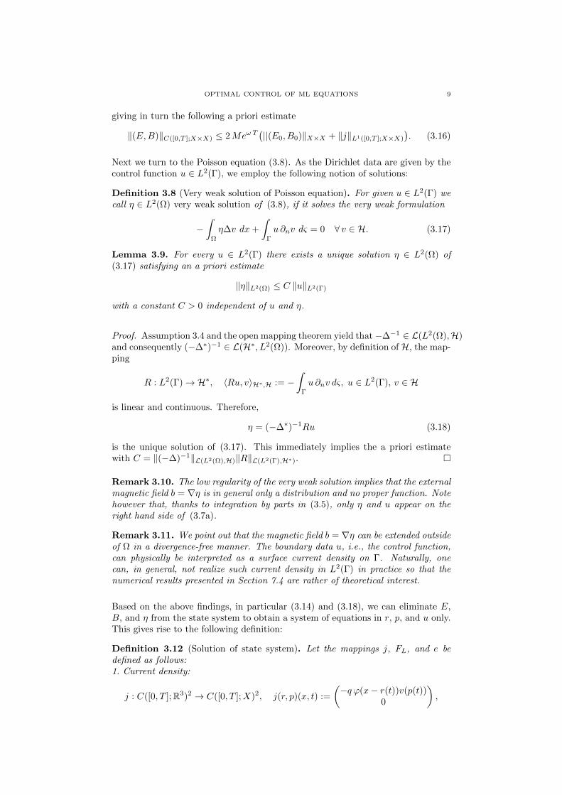
Next we turn to the Poisson equation (3.8). As the Dirichlet data are given by thecontrol function u ∈ L2(Γ), we employ the following notion of solutions:
Definition 3.8 (Very weak solution of Poisson equation). For given u ∈ L2(Γ) wecall η ∈ L2(Ω) very weak solution of (3.8), if it solves the very weak formulation
−ˆ
Ω
η∆v dx+
ˆΓ
u ∂nv dς = 0 ∀ v ∈ H. (3.17)
Lemma 3.9. For every u ∈ L2(Γ) there exists a unique solution η ∈ L2(Ω) of(3.17) satisfying an a priori estimate
‖η‖L2(Ω) ≤ C ‖u‖L2(Γ)
with a constant C > 0 independent of u and η.
Proof. Assumption 3.4 and the open mapping theorem yield that−∆−1 ∈ L(L2(Ω),H)and consequently (−∆∗)−1 ∈ L(H∗, L2(Ω)). Moreover, by definition ofH, the map-ping
R : L2(Γ)→ H∗, 〈Ru, v〉H∗,H := −ˆ
Γ
u ∂nv dς, u ∈ L2(Γ), v ∈ H
is linear and continuous. Therefore,
η = (−∆∗)−1Ru (3.18)
is the unique solution of (3.17). This immediately implies the a priori estimatewith C = ‖(−∆)−1‖L(L2(Ω),H)‖R‖L(L2(Γ),H∗).
Remark 3.10. The low regularity of the very weak solution implies that the externalmagnetic field b = ∇η is in general only a distribution and no proper function. Notehowever that, thanks to integration by parts in (3.5), only η and u appear on theright hand side of (3.7a).
Remark 3.11. We point out that the magnetic field b = ∇η can be extended outsideof Ω in a divergence-free manner. The boundary data u, i.e., the control function,can physically be interpreted as a surface current density on Γ. Naturally, onecan, in general, not realize such current density in L2(Γ) in practice so that thenumerical results presented in Section 7.4 are rather of theoretical interest.
Based on the above findings, in particular (3.14) and (3.18), we can eliminate E,B, and η from the state system to obtain a system of equations in r, p, and u only.This gives rise to the following definition:
Definition 3.12 (Solution of state system). Let the mappings j, FL, and e bedefined as follows:1. Current density:
j : C([0, T ];R3)2 → C([0, T ];X)2, j(r, p)(x, t) :=
(−q ϕ(x− r(t))v(p(t))
0
),

10 C. MEYER, S. M. SCHNEPP, AND O. THOMA
2. Lorentz force:
FL : C([0, T ];R3)2 → C([0, T ];X)
FL(r, p)(x, t) := E(x, t) + β(p(t))×B(x, t)
= E(t)
(E0
B0
)+
ˆ t
0
E(t− τ)j(r, p)(τ) dτ
+ β(p(t))×
(B(t)
(E0
B0
)+
ˆ t
0
B(t− τ)j(r, p)(τ) dτ
),
with the components E and B of the semigroup G, see (3.13)
3. State system operator:
e : C10([0, T ];R3)2 × L2(Γ)→ C([0, T ];R3)2, e(w, z, u) :=
(e1(w, z, u)e2(w, z, u)
),
e1(w, z, u)(t) := z(t)− qˆ
Ω
ϕ(x− w(t)− r0)FL(w + r0, z + p0)(t) dx
+ q
ˆΩ
((−∆∗)−1Ru
)[∇ϕ(x− w(t)− r0)× β(z(t) + p0)
]dx
− qˆ
Γ
uϕ(x− w(t)− r0)β(z(t) + p0)× ndς
e2(w, z, u)(t) := w(t)− v(z(t) + p0).
Then we call a triple (w, z, u) ∈ C10([0, T ];R3)2 × L2(Γ) solution of the state
system, if it satisfies e(w, z, u) = 0.
We point out that, due to the smoothness assumptions on ϕ in (3.1) and theregularity of the mild solution, see Definition (3.7), the mappings j, FL, and e indeedpossess the asserted mapping properties. Note that both PDEs, i.e., Maxwell’sequations as well as the Poisson equation, are incorporated into this notion ofsolution by means of the solution operators of the respective PDE in form of (3.14)and (3.18). Therefore we call the equation e(w, z, u) = 0 reduced (state) system, asit only involves the variables w, z, and u.
With this notion of solution to the state system at hand, we are now in the positionto state a mathematically rigorous version of the optimal control problem underconsideration:
min J (w + r0, u)
s.t. w, z ∈ C10([0, T ];R3), u ∈ L2(Γ)
e(w, z, u)(t) = 0 ∀ t ∈ [0, T ]
gi(w(t) + r0) ≤ 0, i = 1, ...,m, ∀ t ∈ [0, T ].
(P)
For the sake of clarity we recall all variables and their meaning in Table 3.1. Hereand in all what follows, we denote the couple (w, z) by y. For completeness we alsolist the adjoint variables arising in the upcoming sections in this table.
4 Analysis of the state equation
We begin the discussion of (P) with an existence and uniqueness result for thereduced state system. To be more precise, we prove that, for every u ∈ L2(Γ),there exists a unique y ∈ C1
0([0, T ];R3)2 such that e(y, u) = 0. The proof is
classical and based on Banach’s contraction principle. It follows the lines of [28]and [42, Section 2.4], where existence and uniqueness is shown for the Abraham

OPTIMAL CONTROL OF ML EQUATIONS 11
Variable Name of quantity
State variablesE electric fieldB magnetic fieldr position of particlep relativistic momentum of particlew normalized particle positionz normalized momentumy := (w, z)η solution of Poisson equationControl variableu boundary data of Poisson equationAdjoint variablesΦ adjoint electric fieldΨ adjoint magnetic field% adjoint particle positionπ adjoint relativistic momentumω := (%, π)χ adjoint Poisson solutionµ Lagrange multiplierFurther variablesj electric currentFL Lorentz forceρ charge densityγ Lorentz factorb external magnetic fielde external electric fieldϕ smeared out delta distribution
Table 3.1. Overview of arising variables
model for the case Ω = R3 and without the Poisson equation for the externalmagnetic field. Let u ∈ L2(Γ) be fix but arbitrary. The constraint e(y, u) = 0 in(P) is equivalent to
y(t) = f(y, u)(t) ∀ t ∈ [0, T ], y(0) = 0, (4.1)
where f = (f1, f2) : C([0, T ];R3)2 → C([0, T ];R3)2 is given by
f1(w, z, u)(t) := q
ˆΩ
ϕ(x− w(t)− r0)FL(w + r0, z + p0)(t) dx
− qˆ
Ω
((−∆∗)−1Ru
)[∇ϕ(x− w(t)− r0)× β(z(t) + p0)
]dx
+ q
ˆΓ
uϕ(x− w(t)− r0)β(z(t) + p0)× ndς
f2(w, z, u)(t) := v(z(t) + p0).
For the rest of this section we suppressed the dependency of f on u, as u is fixedthroughout this section. In order to apply the Banach’s fixed point theorem, weprove the following
12 C. MEYER, S. M. SCHNEPP, AND O. THOMA
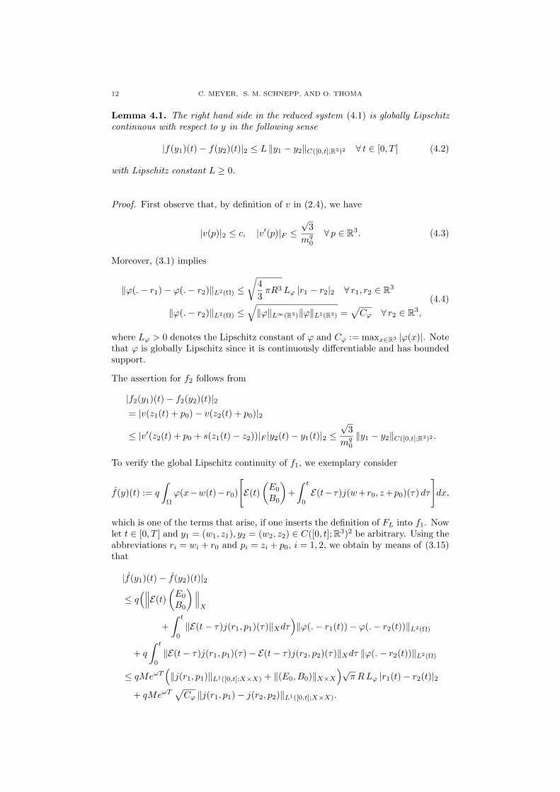
Lemma 4.1. The right hand side in the reduced system (4.1) is globally Lipschitzcontinuous with respect to y in the following sense
|f(y1)(t)− f(y2)(t)|2 ≤ L ‖y1 − y2‖C([0,t];R3)2 ∀ t ∈ [0, T ] (4.2)
with Lipschitz constant L ≥ 0.
Proof. First observe that, by definition of v in (2.4), we have
|v(p)|2 ≤ c, |v′(p)|F ≤√
3
mq0
∀ p ∈ R3. (4.3)
Moreover, (3.1) implies
‖ϕ(.− r1)− ϕ(.− r2)‖L2(Ω) ≤√
4
3πR3 Lϕ |r1 − r2|2 ∀ r1, r2 ∈ R3
‖ϕ(.− r2)‖L2(Ω) ≤√‖ϕ‖L∞(R3)‖ϕ‖L1(R3) =
√Cϕ ∀ r2 ∈ R3,
(4.4)
where Lϕ > 0 denotes the Lipschitz constant of ϕ and Cϕ := maxx∈R3 |ϕ(x)|. Notethat ϕ is globally Lipschitz since it is continuously differentiable and has boundedsupport.
The assertion for f2 follows from
|f2(y1)(t)− f2(y2)(t)|2= |v(z1(t) + p0)− v(z2(t) + p0)|2
≤ |v′(z2(t) + p0 + s(z1(t)− z2))|F |y2(t)− y1(t)|2 ≤√
3
mq0
‖y1 − y2‖C([0,t];R3)2 .
To verify the global Lipschitz continuity of f1, we exemplary consider
f(y)(t) := q
ˆΩ
ϕ(x−w(t)−r0)
[E(t)
(E0
B0
)+
ˆ t
0
E(t− τ)j(w+r0, z+p0)(τ) dτ
]dx,
which is one of the terms that arise, if one inserts the definition of FL into f1. Nowlet t ∈ [0, T ] and y1 = (w1, z1), y2 = (w2, z2) ∈ C([0, t];R3)2 be arbitrary. Using theabbreviations ri = wi + r0 and pi = zi + p0, i = 1, 2, we obtain by means of (3.15)that
|f(y1)(t)− f(y2)(t)|2
≤ q(∥∥∥E(t)
(E0
B0
)∥∥∥X
+
ˆ t
0
‖E(t− τ)j(r1, p1)(τ)‖Xdτ)‖ϕ(.− r1(t))− ϕ(.− r2(t))‖L2(Ω)
+ q
ˆ t
0
‖E(t− τ)j(r1, p1)(τ)− E(t− τ)j(r2, p2)(τ)‖Xdτ ‖ϕ(.− r2(t))‖L2(Ω)
≤ qMeωT(‖j(r1, p1)‖L1([0,t];X×X) + ‖(E0, B0)‖X×X
)√π RLϕ |r1(t)− r2(t)|2
+ qMeωT√Cϕ ‖j(r1, p1)− j(r2, p2)‖L1([0,t];X×X).

OPTIMAL CONTROL OF ML EQUATIONS 13
Concerning the expressions involving j, we find by employing (4.3) and (4.4) that
‖j(r1, p1)− j(r2, p2)‖L1([0,t];X×X)
= q
ˆ t
0
‖ϕ(.− r1(τ))v(p1(τ))− ϕ(.− r2(τ))v(p2(τ))‖Xdτ
≤ qˆ t
0
(‖ϕ(.− r1(τ))− ϕ(.− r2(τ))‖L2(Ω)|v(p1(τ))|2
+ ‖ϕ(.− r2(τ))‖L2(Ω)|v(p1(τ))− v(p2(τ))|2)dτ
≤ q T(√
π RLϕ c ‖r1 − r2‖C([0,t];R3) +√Cϕ
√3
mq0
‖p1 − p2‖C([0,t];R3)
)and
‖j(r1, p1)‖L1([0,t];X×X) = q
ˆ t
0
‖ϕ(.− r1(τ))‖L2(Ω) |v(p1(τ))|2dτ
≤ q T√Cϕ c.
(4.5)
By inserting these estimates we end up with
|f(y1)(t)− f(y2)(t)| ≤ K(‖r1 − r2‖C([0,t];R3) + ‖p1 − p2‖C([0,t];R3)
)≤√
2K ‖y1 − y2‖C([0,t];R3)2
with a constant K > 0 independent of t, y1, and y2. The Lipschitz continuity ofthe remaining parts in f1 can be proven by similar estimates.
Remark 4.2. We point out that the Lipschitz constant in (4.2) depends on u sothat one should rather write
|f(y1, u)(t)− f(y2, u)(t)|2 ≤ L(u) ‖y1 − y2‖C([0,t];R3)2 ∀ t ∈ [0, T ].
Of course, the proof of existence of a solution to (4.1) for fixed u is not affected bythis dependency.
Based on the Lipschitz-estimate in Lemma 4.1, existence and uniqueness can nowbe shown by Banach’s contraction principle. The arguments are classical and followthe lines of [42, Section 2.4]. For convenience of the reader we sketch the proof inAppendix A.
Theorem 4.3. For all u ∈ L2(Γ) there exists a unique solution y ∈ C10([0, T ];R3)2
of the reduced system (4.1) and the following a priori estimate is fulfilled
‖y‖C1([0,T ];R3)2 ≤ C1 ‖u‖L2(Γ) + C2
with a constants C1, C2 > 0 independent of u and y.
5 Existence of an optimal control
With the existence result for the reduced state system in Theorem 4.3 at hand, itis now straightforward to establish the existence of a globally optimal control.
Theorem 5.1. Assume that there is a control u ∈ L2(Γ) such that the associatedstate y = (w, z) ∈ C1
0([0, T ];R3)2 satisfies the state constraint gi(w(t) + r0) ≤ 0
for all i = 1, ...,m and all t ∈ [0, T ]. Then there exists at least one globally optimalcontrol for (P).

14 C. MEYER, S. M. SCHNEPP, AND O. THOMA
Proof. By assumption the feasible set of (P) is non-empty. Thus there existsa minimizing sequence yn, un = wn, zn, un ⊂ C1
0([0, T ];R3)2 × L2(Γ), i.e.,
e(yn, un) = 0, wn(t) + r0 ∈ Ω for all t ∈ [0, T ], and
J (wn + r0, un)n→∞−→ inf (P) =: j ∈ R ∪ −∞.
From Assumption 3.6 we deduce
α
2‖un‖2L2(Γ) ≤ J (wn + r0, un)− c1 T − c2
so that un is bounded in L2(Γ). As e(yn, un) = 0, Theorem 4.3 yields the bound-edness of yn in H1([0, T ];R3)2. Consequently, there exist weakly convergingsubsequences, and w.l.o.g. we assume weak convergence of the whole sequences, i.e.
un u∗ in L2(Γ) and yn y∗ = (w∗, z∗) in H1(]0, T [;R3)2.
The compactness of the embedding H1(]0, T [;R3)2 → C([0, T ];R3)2 then yieldsstrong convergence of yn in the maximum-norm so that Lemma 4.1 and Remark4.2 give
‖f(yn, u∗)− f(y∗, u∗)‖C([0,T ];R3)2 ≤ L(u∗) ‖yn − y∗‖C([0,T ];R3)2
n→∞−→ 0.
Moreover, the strong convergence of the state in C([0, T ];R3)2 further implies
‖β(pn)− β(p∗)‖C([0,T ];R3) → 0, ‖ϕ(.− rn)− ϕ(.− r∗)‖C([0,T ];H1(Ω)) → 0.
As the control only appears linearly in the state system, these convergences allowto pass to the limit in the reduced state equation in weak form, i.e., for everyv = (v1, v2) ∈ L2(0, T ;R3)2 there holdsˆ T
0
y∗(t) · v(t) dt
= limn→∞
ˆ T
0
yn(t) · v(t) dt
= limn→∞
ˆ T
0
f(yn, un)(t) · v(t) dt
= limn→∞
(ˆ T
0
f(yn, u∗)(t) · v(t) dt
− qˆ
Ω
((−∆∗)−1R(un − u∗)
)ˆ T
0
[∇ϕ(x− rn(t))× β(pn(t))
]· v1(t)dt dx
+ q
ˆΓ
(un − u∗)ˆ T
0
[ϕ(x− rn(t))β(pn(t))× n
]· v1(t)dt dς
)
=
ˆ T
0
f(y∗, u∗)(t) · v(t) dt.
Therefore, we obtain
y∗(t) = f(y∗, u∗)(t) f.a.a. t ∈ [0, T ].
Because of y∗ ∈ C([0, T ];R3)2 the right hand side is continuous such that y∗ ∈C1([0, T ];R3)2. From yn → y∗ in C([0, T ];R3)2 we further infer that y∗(0) = 0,and consequently y∗ coincides with the unique solution of (4.1) associated with u∗.The convergence of the state in C([0, T ];R3)2 and the continuity of gi, i = 1, ...,m,moreover yield
gi(w∗(t) + r0) ≤ 0 ∀ i = 1, ...,m ⇔ w∗(t) + r0 ∈ Ω

OPTIMAL CONTROL OF ML EQUATIONS 15
for all t ∈ [0, T ] such that the state constraint is also fulfilled in the limit. Therefore,the couple (y∗, u∗) fulfills all constraints in (P).
Finally, the strong convergence of yn in C([0, T ];R3)2, the weak convergence ofun in L2(Γ), and the weak lower semicontinuity of ‖.‖2L2(Γ) allow to pass to the
limit in the objective:
j = limn→∞
J (wn + r0, un)
≥ limn→∞
( ˆ T
0
J1(wn(t) + r0) dt+ J2(wn(T ) + r0))
+ lim infn→∞
α
2
ˆΓ
u2n dς
≥ J (w∗ + r0, u∗),
which implies the optimality of (y∗, u∗).
6 First-order necessary optimality conditions
For the rest of the paper, we slightly change the functional analytical framework ofthe optimal control problem under consideration. To be more precise, we weakenthe regularity of the state space in order to obtain a more regular adjoint state andtreat the state as a function in
Y = y ∈ H1(]0, T [;R3)2 : y(0) = 0.
Thus the mapping associated with the reduced state system becomes e : Y ×L2(Γ)→ Z = L2(]0, T [;R3)2, with a slight abuse of notation still denoted by e. Itis easily seen that this modification does not affect the above analysis, in particularthe proof of existence of an optimal control, since the state is treated as a functionin H1(]0, T [;R3)2 there anyway. Note that H1(]0, T [;R3)2 → C([0, T ];R3)2 so thatthe mappings j and FL from Definition 3.12 are still well-defined.
Remark 6.1. If a couple (y, u) ∈ Y × L2(Γ) satisfies the constraint e(y, u) = 0,i.e.,
y(t) = f(y, u)(t) f.a.a. t ∈ [0, T ], y(0) = 0,
then f(y, u) ∈ C([0, T ];R3)2 implies y ∈ C1([0, T ];R3)2 so that y coincides with theunique solution of (4.1) from Theorem 4.3. In other words, the treatment of (P)in the weaker state space Y does not affect the regularity of the optimal state.
6.1. The linearized state equation. We start the derivation of a qualified op-timality system by the analysis of the linearized reduced state system.
Lemma 6.2. The reduced form e is continuously Frechet-differentiable from Y ×L2(Γ) to Z. Its partial derivatives at (y, u) = (w, z, u) ∈ Y × L2(Γ) in direction(φ, h) = (φr, φp, h) ∈ Y × L2(Γ) are given by(∂e1
∂y(y, u)φ
)(t) = φp(t)−
(∂f1
∂y(y, u)φ
)(t),(∂e2
∂y(y, u)φ
)(t) = φr(t)−
(∂f2
∂y(y, u)φ
)(t),(∂e1
∂u(y, u)h
)(t) = −
(∂f1
∂u(y, u)h
)(t),
(∂e1
∂u(y, u)h
)(t) = 0

16 C. MEYER, S. M. SCHNEPP, AND O. THOMA
with(∂f1
∂u(y, u)h
)(t) = q
ˆΓ
hϕ(x− r(t))β(p(t))× ndς
− qˆ
Ω
(−∆∗)−1Rh[∇ϕ(x− r(t))× β(p(t))] dx,(∂f2
∂y(y, u)φ
)(t) = v′(p(t))φp(t),
and(∂f1
∂y(y, u)φ
)(t) = −q
ˆΩ
[∇ϕ(x− r(t)) · φr(t)
]FL(r, p)(t) dx
+ q
ˆΩ
ϕ(x− r(t))(∂yFL(r, p)φ
)(t) dx
+ q
ˆΓ
u[ϕ(x− r(t))β′(p(t))φp(t)
−[∇ϕ(x− r(t)) · φr(t)
]β(p(t))
]× ndς
+ q
ˆΩ
((−∆∗)−1Ru
) [∇2ϕ(x− r(t))φr(t)× β(p(t))
−∇ϕ(x− r(t))× β′(p(t))φp(t)]dx,
with r = w + r0, p = z + p0, the derivative of the Lorentz force term FL(∂yFL(r, p)φ
)(t) =
(∂rFL(r, p)φr + ∂pFL(r, p)φp
)(t)
=
ˆ t
0
E(t− τ)(j′(r, p)(τ)φ(τ)
)dτ
+ β(p(t))׈ t
0
B(t− τ)(j′(r, p)(τ)φ(τ)
)dτ
+ β′(p(t))φp(t)×
(B(t)
(E0
B0
)+
ˆ t
0
B(t− τ)j(r, p)(τ) dτ
)and j′ as given in (3.11).
Proof. As a linear and bounded operator the time derivative is clearly continuouslyFrechet-differentiable for H1(]0, T [;R3) to L2(]0, T [;R3). All nonlinear Nemyzki-operators involved in f are differentiated in spaces of continuous functions. Becauseof its slightly non-standard structure, we exemplary study the Frechet-differentiabilityof r 7→ ∇ϕ(.− r) from C([0, T ];R3) to C([0, T ];L2(Ω)):
‖∇ϕ(.− (r + φr))−∇ϕ(.− r)−∇2ϕ(.− r) · φr‖2C([0,T ];L2(Ω))
= maxt∈[0,T ]
( ˆΩ
|∇ϕ(x− r(t)− φr(t))−∇ϕ(x− r(t))−∇2ϕ(x− r(t))φr(t)|2 dx
= maxt∈[0,T ]
ˆΩ
∣∣∣ˆ 1
0
∇2ϕ(x− r(t)− θφr(t)
)φr(t)dθ −∇2ϕ(x− r(t))φr(t)
∣∣∣2 dx≤ maxt∈[0,T ]
ˆΩ
∣∣∣ˆ 1
0
Lϕ,2 θ |φr(t)|2dθ∣∣∣2dx =
1
4L2ϕ,2 |Ω| ‖φr(t)‖4C([0,T ];R3),
where Lϕ,2 denotes the Lipschitz constant of ∇2ϕ. This gives the partial dif-ferentiability of f w.r.t. y. As u only appears linearly, f is moreover partiallydifferentiable w.r.t. u. Furthermore, one readily verifies that these partial deriva-tives are continuous in (y, u). Therefore, [8, Theorem 3.7.1] gives the continuousFrechet-differentiability of e.

OPTIMAL CONTROL OF ML EQUATIONS 17
Lemma 6.3. Let (y, u) ∈ Y ×L2(Γ) be given. Then for every h ∈ Z there exists aunique solution φ = (φr, φp) ∈ Y of the linearized equation
∂e
∂y(y, u)φ = h. (6.1)
Proof. In view of Lemma 6.2, (6.1) is equivalent to(φp(t)
φr(t)
)=(∂f∂y
(y, u)φ)
(t) + h(t) f.a.a. t ∈ [0, T ], φ(0) = 0
with ∂yf(y, u)φ = (∂yf1(y, u)φ, ∂yf2(y, u)φ). As in the proof of Theorem 4.3, exis-tence and uniqueness of the equivalent integral equation, given by(
φp(t)φr(t)
)=
ˆ t
0
[(∂f∂y
(y, u)φ)
(τ) + h(τ)]dτ,
can again be proven by Banach’s contraction principle, provided that there is aconstant C > 0 such that∣∣∣(∂f
∂y(y, u)φ
)(t)∣∣∣2≤ C ‖φ‖C([0,t];R3)2 ∀ t ∈ [0, T ],
cf. (4.2). (Note in this context that φ 7→ ∂yf(y, u)φ is a linear mapping so thatLipschitz continuity is equivalent to boundedness.) The latter inequality howevercan be verified by estimates similar to the proof of Lemma 4.1.
6.2. KKT conditions. Having established the differentiability of the reducedstate system, we are now in the position to derive first-order optimality systemin qualified form, i.e., Karush-Kuhn-Tucker (KKT) conditions involving Lagrangemultipliers associated with the constraints in (P). To this end, let (y∗, u∗) =(w∗, z∗, u∗) ∈ Y × L2(Γ) be a arbitrary local optimum of (P). As before, we setr∗ = w∗+ r0 and p∗ = z∗+ p0 in all what follows. It is known that the existence ofLagrange multipliers requires certain constraint qualifications, see e.g. [51]. In ourcase, one of these, namely the surjectivity of ∂ye(y
∗, u∗), was established in Lemma6.3. However, we need an additional condition to obtain a Lagrange multiplier forthe pointwise state constraint in (P), too.
Assumption 6.4 (Linearized Slater condition). We assume that there is a function
h ∈ L2(Γ) so that
gi(r∗(t)) + g′i(r
∗(t))φr(t) < 0 ∀ t ∈ [0, T ], i = 1, ...,m, (6.2)
where φ = (φr, φp) ∈ Y is the solution to (6.1) for h = h.
Note that the Nemyzki operators associated with g1, ..., gm are Frechet-differentiablefrom C([0, T ];R3) to C([0, T ]) by Assumption 3.6. The same holds for the functionsJ1 and J2 within the objective.
Given that Assumption 6.4 is fulfilled, one can establish the existence of Lagrangemultipliers, see for instance [25, Section 1.7.3.4]. To be more precise, under As-sumption 6.4 there exists (π, %, λ) ∈ Z × C([0, T ];Rm)∗ such that the following
18 C. MEYER, S. M. SCHNEPP, AND O. THOMA
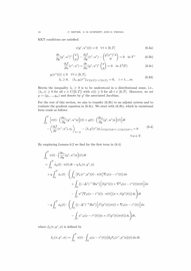
KKT conditions are satisfied:
e(y∗, u∗)(t) = 0 ∀ t ∈ [0, T ] (6.3a)
∂e
∂y(y∗, u∗)∗
(π%
)− ∂J∂y
(r∗, u∗)−(g′(r∗)∗λ
0
)= 0 in Y ∗ (6.3b)
∂J∂u
(r∗, u∗) +∂e
∂u(y∗, u∗)∗
(π%
)= 0 in L2(Γ) (6.3c)
gi(r∗(t)) ≤ 0 ∀ t ∈ [0, T ],
λi ≥ 0, 〈λi, gi(r∗)〉C([0,T ])∗,C([0,T ]) = 0, i = 1, ...m.(6.3d)
Herein the inequality λi ≥ 0 is to be understood in a distributional sense, i.e.,〈λi, v〉 ≥ 0 for all v ∈ C([0, T ]) with v(t) ≥ 0 for all t ∈ [0, T ]. Moreover, we setg := (g1, ..., gm) and denote by g′ the associated Jacobian.
For the rest of this section, we aim to transfer (6.3b) to an adjoint system and toevaluate the gradient equation in (6.3c). We start with (6.3b), which in variationalform reads as follows
ˆ T
0
[π(t) ·
(∂e1
∂y(y∗, u∗)φ
)(t) + %(t) ·
(∂e2
∂y(y∗, u∗)φ
)(t)]dt
−⟨∂J∂r
(r∗, u∗), φr
⟩Y ∗,Y
− 〈λ, g′(r∗)φr〉C([0,T ];Rm)∗,C([0,T ];Rm) = 0
∀φ ∈ Y.
(6.4)
By employing Lemma 6.2 we find for the first term in (6.4)
ˆ T
0
π(t) ·(∂e1
∂y(y∗, u∗)φ
)(t) dt
=
ˆ T
0
φp(t) · π(t) dt− q IL(π, y∗, φ)
+ q
ˆ T
0
φr(t) ·
( ˆΩ
[FL(r∗, p∗)(t) · π(t)
]∇ϕ(x− r∗(t)) dx
+
ˆΩ
((−∆∗)−1Ru∗
)[β(p∗(t))×∇2ϕ(x− r∗(t))π(t)
]dx
−ˆ
Γ
u∗[∇ϕ(x− r∗(t)) · π(t)
](n× β(p∗(t))
)dς
)dt
− qˆ T
0
φp(t) ·
( ˆΩ
((−∆∗)−1Ru∗
)[β′(p∗(t))π(t)×∇ϕ(x− r∗(t))
]dx
−ˆ
Γ
u∗ ϕ(x− r∗(t))(n× β′(p∗(t))π(t)
)dς
)dt,
where IL(π, y∗, φ) is defined by
IL(π, y∗, φ) :=
ˆ T
0
π(t) ·ˆ
Ω
ϕ(x− r∗(t))(∂yFL(r∗, p∗)φ
)(t) dx dt.

OPTIMAL CONTROL OF ML EQUATIONS 19
In view of Lemma 6.2, applying Fubini’s theorem to this expression leads to
IL(π, y∗, φ)
=
ˆ T
0
ˆ t
0
ˆΩ
[E(t− τ)
(j′(r∗, p∗)(τ)φ(τ)
)+ β(p∗(t))× B(t− τ)
(j′(r∗, p∗)(τ)φ(τ)
)]· ϕ(x− r∗(t))π(t) dx dτ dt
+
ˆ T
0
ˆΩ
ϕ(x− r∗(t))β′(p(t))φp(t)×B∗(t) · π(t) dx dt
=
ˆ T
0
φ(t) ·ˆ
Ω
j′(r∗, p∗)(t)>ˆ T
t
G(τ − t)∗κ(r∗, p∗, π)(τ) dτ dx dt
+
ˆ T
0
φp(t) ·ˆ
Ω
B∗(t)× ϕ(x− r∗(t))β′(p∗(t))π(t) dx dt,
where we abbreviated
B∗(t) := B(t)
(E0
B0
)+
ˆ t
0
B(t− τ)j(r, p)(τ) dτ
and set
κ : R3 × R3 × R3 → R3 × R3
κ(r, p, π) :=
(ϕ(x− r)π
π × ϕ(x− r)β(p)
).
Moreover let us define(Φ(t)Ψ(t)
):=
ˆ T
t
G(τ − t)∗κ(r∗, p∗, π)(τ) dτ (6.5)
Since −iA is self-adjoint, the theorem of Stone implies that G(t)∗ is the semigroupgenerated by the adjoint operator
A∗ : X ×X → X ×X, A∗ =
(0 curl
− curl 0
)with domain D(A∗) = D(A) = HΓ
curl. Thus (Φ,Ψ) ∈ C([0, T ];X)2 is the mildsolution of the following backward-in-time problem:
− ∂
∂t
(Φ(t)Ψ(t)
)+A∗
(Φ(t)Ψ(t)
)=
(ϕ( . − r∗(t))π(t)
π(t)× ϕ( . − r∗(t))β(p∗(t))
)Φ(T ) = Ψ(T ) = 0.
(6.6)
By setting ω := (%, π) and summarizing the above transformations, we obtain forthe first two addends in (6.4)
ˆ T
0
[π(t) ·
(∂e1
∂y(y∗, u∗)φ
)(t) + %(t) ·
(∂e2
∂y(y∗, u∗)φ
)(t)]dt
=
ˆ T
0
φ(t) · ω(t) dt+
ˆ T
0
φ(t) ·A(y∗, u∗, ω)(t) dt

20 C. MEYER, S. M. SCHNEPP, AND O. THOMA
with
A(y∗, u∗, ω)(t) =
(Ar(y
∗, u∗, ω)(t)Ap(y
∗, u∗, ω)(t)
):= q
( ´Ω
[FL(r∗, p∗)(t) · π(t)
]∇ϕ(x− r∗(t)) dx
−´
ΩB∗(t)× ϕ(x− r∗(t))β′(p∗(t))π(t) dx
)
+ q
´Ω η∗[β(p∗(t))×∇2ϕ(x− r∗(t))π(t)
]dx
−´
Ωη∗[β′(p∗(t))π(t)×∇ϕ(x− r∗(t))
]dx
+ q
(−´
Γu∗[∇ϕ(x− r∗(t)) · π(t)
](n× β(p∗(t))
)dς´
Γu∗ ϕ(x− r∗(t))
(n× β′(p∗(t))π(t)
)dς
)
+ q2
(−´
Ωv(p∗(t))
[∇ϕ(x− r∗(t)) · Φ(t)
]dx´
Ωϕ(x− r∗(t)) v′(p∗(t))Φ(t) dx
)−(
0v′(p∗(t))%(t)
),
(6.7)
where η∗ = (−∆∗)−1Ru∗. Thus the adjoint equation (6.4) becomes
ˆ T
0
φ(t) · ω(t) dt+
ˆ T
0
φ(t) ·A(y∗, u∗, ω)(t) dt−⟨∂J∂r
(r∗, u∗), φr
⟩Y ∗,Y
−〈λ, g′(r∗)φr〉C([0,T ];Rm)∗,C([0,T ];Rm) = 0 ∀φ ∈Y.(6.8)
By the Riesz representation theorem λ ∈ C([0, T ];Rm)∗ can be identified with afunction of bounded variations. This leads to the following result, whose detailedproof is given in Appendix B.
Lemma 6.5. The adjoint particle position % and the adjoint momentum π sat-isfy % ∈ BV([0, T ];R3) and π ∈ W 1,∞(]0, T [;R3). Together with a function µ ∈NBV([0, T ];Rm) they fulfill the following ODEs backward in time:
−π(t) = −Ap(y∗, u∗, %, π)(t) a.e. in ]0, T [ (6.9)
π(T ) = 0 (6.10)
−%(t) = −Ar(y∗, u∗, %, π)(t) +∇J1(r∗(t))− g′(r∗(t))>µ(t) a.e. in ]0, T [ (6.11)
%(T ) = ∇J2(r∗(T )). (6.12)
In addition, µ is monotone increasing and satisfies
ˆ T
0
g(r∗(t)) · dµ(t) = 0.
Moreover, % only admits finitely many points of discontinuity t1, ..., t` in ]0, T [, ateach of which
%(ti)− limε0
%(ti − ε) = g′(r∗(ti))>( lim
ε0µ(ti − ε)− µ(ti)
), i = 1, ..., `, (6.13)
holds true.
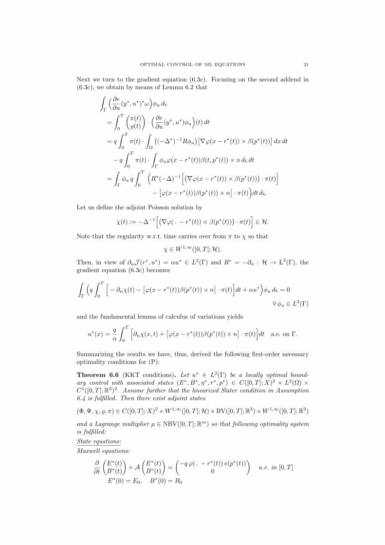
OPTIMAL CONTROL OF ML EQUATIONS 21
Next we turn to the gradient equation (6.3c). Focusing on the second addend in(6.3c), we obtain by means of Lemma 6.2 that
ˆΓ
( ∂e∂u
(y∗, u∗)∗ω)φu dς
=
ˆ T
0
(π(t)%(t)
)·( ∂e∂u
(y∗, u∗)φu
)(t) dt
= q
ˆ T
0
π(t) ·ˆ
Ω
((−∆∗)−1Rφu
)[∇ϕ(x− r∗(t))× β(p∗(t))
]dx dt
− qˆ T
0
π(t) ·ˆ
Γ
φuϕ(x− r∗(t))β(t, p∗(t))× ndς dt
=
ˆΓ
φu q
ˆ T
0
(R∗(−∆)−1
[(∇ϕ(x− r∗(t))× β(p∗(t))
)· π(t)
]−[ϕ(x− r∗(t))β(p∗(t))× n
]· π(t)
)dt dς.
Let us define the adjoint Poisson solution by
χ(t) := −∆−1[(∇ϕ( . − r∗(t))× β(p∗(t))
)· π(t)
]∈ H.
Note that the regularity w.r.t. time carries over from π to χ so that
χ ∈W 1,∞(]0, T [;H).
Then, in view of ∂uJ (r∗, u∗) = αu∗ ∈ L2(Γ) and R∗ = −∂n : H → L2(Γ), thegradient equation (6.3c) becomes
ˆΓ
(q
ˆ T
0
[− ∂nχ(t)−
[ϕ(x− r∗(t))β(p∗(t))× n
]· π(t)
]dt+ αu∗
)φu dς = 0
∀φu ∈ L2(Γ)
and the fundamental lemma of calculus of variations yields
u∗(x) =q
α
ˆ T
0
[∂nχ(x, t) +
[ϕ(x− r∗(t))β(p∗(t))× n
]· π(t)
]dt a.e. on Γ.
Summarizing the results we have, thus, derived the following first-order necessaryoptimality conditions for (P):
Theorem 6.6 (KKT conditions). Let u∗ ∈ L2(Γ) be a locally optimal bound-ary control with associated states (E∗, B∗, η∗, r∗, p∗) ∈ C([0, T ];X)2 × L2(Ω) ×C1([0, T ];R3)2. Assume further that the linearized Slater condition in Assumption6.4 is fulfilled. Then there exist adjoint states
(Φ,Ψ, χ, %, π) ∈ C([0, T ];X)2×W 1,∞(]0, T [;H)×BV([0, T ];R3)×W 1,∞([0, T ];R3)
and a Lagrange multiplier µ ∈ NBV([0, T ];Rm) so that following optimality systemis fulfilled:
State equations:
Maxwell equations:
∂
∂t
(E∗(t)B∗(t)
)+A
(E∗(t)B∗(t)
)=
(−q ϕ( . − r∗(t)) v(p∗(t))
0
)a.e. in [0, T ]
E∗(0) = E0, B∗(0) = B0
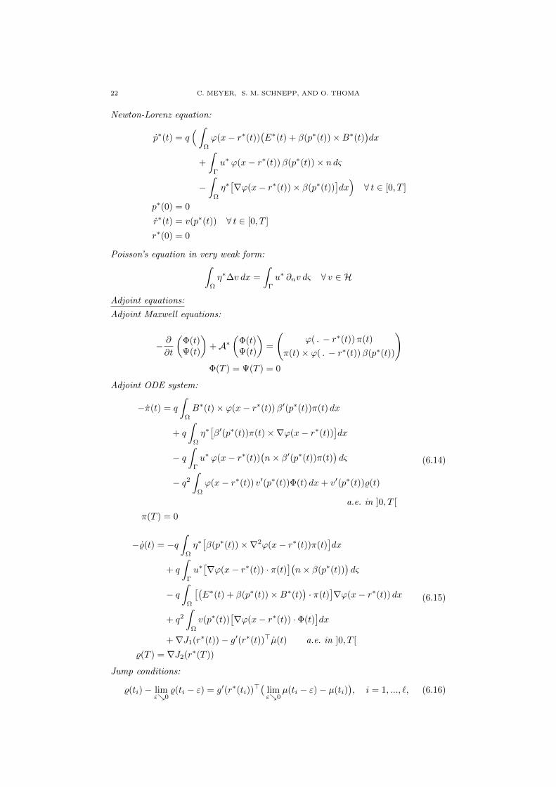
22 C. MEYER, S. M. SCHNEPP, AND O. THOMA
Newton-Lorenz equation:
p∗(t) = q(ˆ
Ω
ϕ(x− r∗(t))(E∗(t) + β(p∗(t))×B∗(t)
)dx
+
ˆΓ
u∗ ϕ(x− r∗(t))β(p∗(t))× ndς
−ˆ
Ω
η∗[∇ϕ(x− r∗(t))× β(p∗(t))
]dx)∀ t ∈ [0, T ]
p∗(0) = 0
r∗(t) = v(p∗(t)) ∀ t ∈ [0, T ]
r∗(0) = 0
Poisson’s equation in very weak form:ˆΩ
η∗∆v dx =
ˆΓ
u∗ ∂nv dς ∀ v ∈ H
Adjoint equations:
Adjoint Maxwell equations:
− ∂
∂t
(Φ(t)Ψ(t)
)+A∗
(Φ(t)Ψ(t)
)=
(ϕ( . − r∗(t))π(t)
π(t)× ϕ( . − r∗(t))β(p∗(t))
)Φ(T ) = Ψ(T ) = 0
Adjoint ODE system:
−π(t) = q
ˆΩ
B∗(t)× ϕ(x− r∗(t))β′(p∗(t))π(t) dx
+ q
ˆΩ
η∗[β′(p∗(t))π(t)×∇ϕ(x− r∗(t))
]dx
− qˆ
Γ
u∗ ϕ(x− r∗(t))(n× β′(p∗(t))π(t)
)dς
− q2
ˆΩ
ϕ(x− r∗(t)) v′(p∗(t))Φ(t) dx+ v′(p∗(t))%(t)
a.e. in ]0, T [
π(T ) = 0
(6.14)
−%(t) = −qˆ
Ω
η∗[β(p∗(t))×∇2ϕ(x− r∗(t))π(t)
]dx
+ q
ˆΓ
u∗[∇ϕ(x− r∗(t)) · π(t)
](n× β(p∗(t))
)dς
− qˆ
Ω
[(E∗(t) + β(p∗(t))×B∗(t)
)· π(t)
]∇ϕ(x− r∗(t)) dx
+ q2
ˆΩ
v(p∗(t))[∇ϕ(x− r∗(t)) · Φ(t)
]dx
+∇J1(r∗(t))− g′(r∗(t))>µ(t) a.e. in ]0, T [
%(T ) = ∇J2(r∗(T ))
(6.15)
Jump conditions:
%(ti)− limε0
%(ti − ε) = g′(r∗(ti))>( lim
ε0µ(ti − ε)− µ(ti)
), i = 1, ..., `, (6.16)

OPTIMAL CONTROL OF ML EQUATIONS 23
Adjoint Poisson equation:
−∆χ(x, t) =(∇ϕ(x− r∗(t))× β(p∗(t))
)· π(t) f.a.a. (x, t) ∈ ]0, T [×Ω
χ(x, t) = 0 f.a.a. (x, t) ∈ ]0, T [×Γ
Gradient equation:
u∗(x) =q
α
ˆ T
0
[∂nχ(x, t) +
[ϕ(x− r∗(t))β(p∗(t))× n
]· π(t)
]dt a.e. on Γ
Complementary relations:
µj monotone increasing,
ˆ T
0
gj(r∗(t)) dµj(t) = 0, gj(r
∗(t)) ≤ 0 ∀ t ∈ [0, T ]
for all j = 1, ..,m
Remark 6.7. As a function of bounded variation, µ can be decomposed as
µ = µa + µd + µs,
where µa ∈ AC([0, T ];Rm) is absolutely continuous and µd ∈ L∞(]0, T [;Rm) isa step function covering the discontinuities of µ. Moreover, µs ∈ C([0, T ];Rm)is the singular part, which is non-constant and whose derivative vanishes almosteverywhere. Consequently, µ in (6.15) can be replaced by µa, while (6.16) holdsalso with µd instead of µ.
Remark 6.8. By integration by parts one can formally derive a strong formulationof the adjoint Maxwell equations in Theorem 6.6:
− ∂
∂tΦ(x, t) + curl Ψ(x, t) = ϕ(x− r∗(t))π(t) in Ω× [0, T ]
(6.17)
− ∂
∂tΨ(x, t)− curl Φ(x, t) = π(t)× ϕ(x− r∗(t))β(p∗(t)) in Ω× [0, T ]
(6.18)
div( ∂∂t
Φ(x, t))
= −div(ϕ(x− r∗(t))π(t)
)in Ω× [0, T ]
(6.19)
div( ∂∂t
Ψ(x, t))
= −div(π(t)× ϕ(x− r∗(t))β(p∗(t))
)in Ω× [0, T ]
(6.20)
Φ(ς, t)× n = 0,∂
∂tΨ(ς, t) · n = −π(t)× ϕ(ς − r∗(t)β(p∗(t))) · n in Γ× [0, T ]
(6.21)
Φ(x, T ) = 0, Ψ(x, T ) = 0 in Ω. (6.22)
Note that the right hand side in (6.17)–(6.18) does, in general, not satisfy a conser-vation of charge, which gives rise to non-standard equations in (6.19) and (6.20)and the unusual boundary condition in (6.21).
7 Numerical investigations
In the following we illustrate by means of a representative example that the optimalcontrol problem (P) can be treated numerically. We follow the analytical approachand use the reduced state system of Definition 3.12 for our numerical investigations.After a brief description of the numerical method we will present some exemplaryresults.
24 C. MEYER, S. M. SCHNEPP, AND O. THOMA
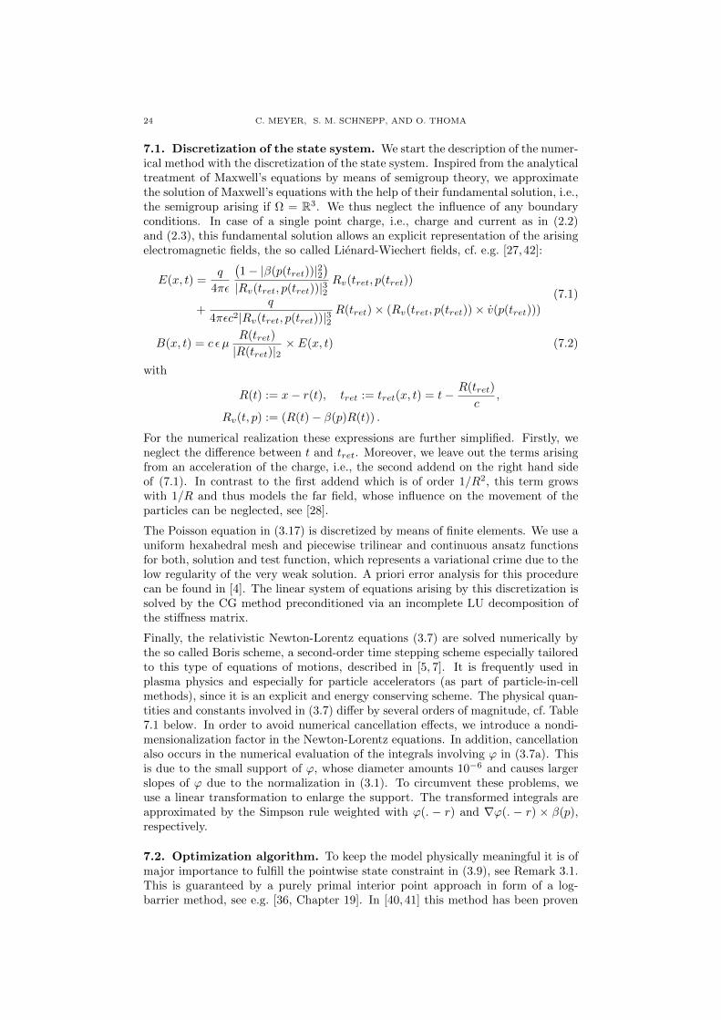
7.1. Discretization of the state system. We start the description of the numer-ical method with the discretization of the state system. Inspired from the analyticaltreatment of Maxwell’s equations by means of semigroup theory, we approximatethe solution of Maxwell’s equations with the help of their fundamental solution, i.e.,the semigroup arising if Ω = R3. We thus neglect the influence of any boundaryconditions. In case of a single point charge, i.e., charge and current as in (2.2)and (2.3), this fundamental solution allows an explicit representation of the arisingelectromagnetic fields, the so called Lienard-Wiechert fields, cf. e.g. [27, 42]:
E(x, t) =q
4πε
(1− |β(p(tret))|22
)|Rv(tret, p(tret))|32
Rv(tret, p(tret))
+q
4πεc2|Rv(tret, p(tret))|32R(tret)× (Rv(tret, p(tret))× v(p(tret)))
(7.1)
B(x, t) = c ε µR(tret)
|R(tret)|2× E(x, t) (7.2)
with
R(t) := x− r(t), tret := tret(x, t) = t− R(tret)
c,
Rv(t, p) := (R(t)− β(p)R(t)) .
For the numerical realization these expressions are further simplified. Firstly, weneglect the difference between t and tret. Moreover, we leave out the terms arisingfrom an acceleration of the charge, i.e., the second addend on the right hand sideof (7.1). In contrast to the first addend which is of order 1/R2, this term growswith 1/R and thus models the far field, whose influence on the movement of theparticles can be neglected, see [28].
The Poisson equation in (3.17) is discretized by means of finite elements. We use auniform hexahedral mesh and piecewise trilinear and continuous ansatz functionsfor both, solution and test function, which represents a variational crime due to thelow regularity of the very weak solution. A priori error analysis for this procedurecan be found in [4]. The linear system of equations arising by this discretization issolved by the CG method preconditioned via an incomplete LU decomposition ofthe stiffness matrix.
Finally, the relativistic Newton-Lorentz equations (3.7) are solved numerically bythe so called Boris scheme, a second-order time stepping scheme especially tailoredto this type of equations of motions, described in [5, 7]. It is frequently used inplasma physics and especially for particle accelerators (as part of particle-in-cellmethods), since it is an explicit and energy conserving scheme. The physical quan-tities and constants involved in (3.7) differ by several orders of magnitude, cf. Table7.1 below. In order to avoid numerical cancellation effects, we introduce a nondi-mensionalization factor in the Newton-Lorentz equations. In addition, cancellationalso occurs in the numerical evaluation of the integrals involving ϕ in (3.7a). Thisis due to the small support of ϕ, whose diameter amounts 10−6 and causes largerslopes of ϕ due to the normalization in (3.1). To circumvent these problems, weuse a linear transformation to enlarge the support. The transformed integrals areapproximated by the Simpson rule weighted with ϕ(. − r) and ∇ϕ(. − r) × β(p),respectively.
7.2. Optimization algorithm. To keep the model physically meaningful it is ofmajor importance to fulfill the pointwise state constraint in (3.9), see Remark 3.1.This is guaranteed by a purely primal interior point approach in form of a log-barrier method, see e.g. [36, Chapter 19]. In [40, 41] this method has been proven
OPTIMAL CONTROL OF ML EQUATIONS 25
to work in function space for one dimensional problems, i.e., problems involvingODEs as in our case. The reduction of the homotopy parameter associated withthe primal interior point method follows an update strategy by [36, Section 19.3].
For the optimization algorithm we reduce the optimal control problem to an op-timization problem in the control variable u only, which is justified by Theorem4.3. The major advantage of this procedure is a significant reduction of the num-ber of optimization variables, since the control u is only one dimensional. It doesnot depend on time, and has its support on Γ instead of the whole domain Ω.The dimension of the optimization problem reduced to the control variable, thus,amounts to the number of nodes on the boundary only. This allows to employ opti-mization methods, which require large memory demand like the BFGS method, seee.g. [36, Section 6.1]. Thanks to the reduction of the dimension the BFGS methodcan be run for a moderate number of degrees of freedom on a computer with 4GBRAM without any limited memory modification. In order to globalize the method,we perform a curvature test to switch from the BFGS direction to the negative gra-dient of the objective, if necessary, and apply a line-search according to the Armijorule.
As a consequence of this reduction approach the mapping u 7→ J (r(u), u) as well asits derivative have to be evaluated in every iteration of the optimization algorithm.Here r(u) denotes the r-component of the solution of state system associated withu. The derivative of u 7→ J (r(u), u) is computed numerically by means of theautomatic differentiation tool ADiMat [6]. As the number of control variables ismuch higher than the number of output variables, which is just a real number, weuse the reverse mode. Moreover, we exclude the linear parts of the solution mappingof the state system from automatic differentiation to differentiate them by hand.This especially concerns the iterative solver of Poisson’s equation. To summarizewe thus follow a first-discretize-then optimize approach. It is not clear whetherthe discrete adjoint equation arising in this way can be interpreted as a suitablediscretization of the adjoint system in Theorem 6.6. In particular, the adjoint Borisscheme gives rise to future research with regard to its stability and consistency.
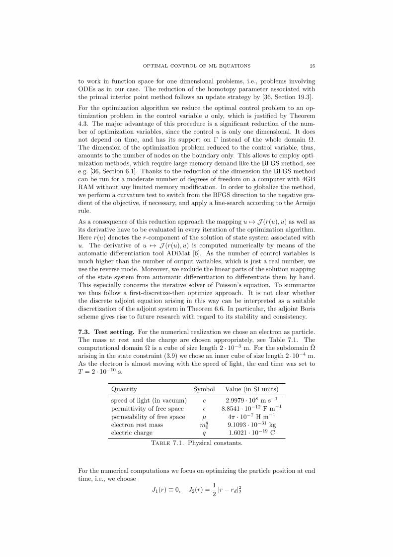
7.3. Test setting. For the numerical realization we chose an electron as particle.The mass at rest and the charge are chosen appropriately, see Table 7.1. Thecomputational domain Ω is a cube of size length 2 · 10−3 m. For the subdomain Ωarising in the state constraint (3.9) we chose an inner cube of size length 2 ·10−4 m.As the electron is almost moving with the speed of light, the end time was set toT = 2 · 10−10 s.
Quantity Symbol Value (in SI units)
speed of light (in vacuum) c 2.9979 · 108 m s−1
permittivity of free space ε 8.8541 · 10−12 F m−1
permeability of free space µ 4π · 10−7 H m−1
electron rest mass mq0 9.1093 · 10−31 kg
electric charge q 1.6021 · 10−19 C
Table 7.1. Physical constants.
For the numerical computations we focus on optimizing the particle position at endtime, i.e., we choose
J1(r) ≡ 0, J2(r) =1
2|r − rd|22

26 C. MEYER, S. M. SCHNEPP, AND O. THOMA
for the contributions to the objective in (P) and (P), respectively. Furthermore,the Tikhonov parameter α in the objective is set to α = 10−9 to compensate for thecomparatively large values of the control. Consequently we are mainly interested insteering the particle beam at a given end time to a fixed position rd. As a stoppingcriterion for the overall algorithm we check if the relative error between the desiredparticle position rd and the computed one is below a given tolerance.
For the computations presented in the following section, we used an equidistantmesh with 17,576 nodes. This amounts to 7,504 nodes on the boundary, i.e., thenumber of unknown control variables, which corresponds to the dimension of theoptimization problem. For the numerical integration of the ODE we used an equidis-tant time step of 10−12 s.
7.4. Numerical results. The particle trajectories for selected iterations of theoptimization algorithms are shown in Figures 7.2 to 7.6. While the particle iscolored in black, we marked the desired end position in the upper left corner ingrey. It is to be noted that the control u only influences the magnetic field, whichin turn cannot slow down or accelerate this particle beam since its contributionto the Lorentz force only acts perpendicular to the direction of motion, cf. (2.6a).This causes spiral shaped trajectories such as the ones depicted in figures 7.1 to 7.6.The desired end position has been reached after 47 iterations of the optimizationalgorithm with an accuracy of 3.5 · 10−8 m.
Figure 7.1. Particletrajectory in iteration 0.
Figure 7.2. Particletrajectory in iteration 1.
The optimal external magnetic field on the boundary of Ω generated by the optimalcontrol u∗ is shown in Figures 7.7 and 7.8.
Table 7.2 shows the convergence history of the globalized BFGS interior pointmethod. Beside the objective value and Euclidean norm of the gradient, Table 7.2shows the used descent direction for selected iterations, where “BFGS” refers tothe BFGS direction and “Grad” is the negative gradient.

OPTIMAL CONTROL OF ML EQUATIONS 27
Figure 7.3. Particletrajectory in iteration 5.
Figure 7.4. Particletrajectory in iteration20.
Figure 7.5. Particletrajectory in iteration40.
Figure 7.6. Particletrajectory in iteration47.
A Proof of Theorem 4.3
Clearly, y solves (4.1) if and only if it is a fixed point of
G : C([0, T ];R3)2 → C([0, T ];R3)2, G(y)(t) :=
ˆ t
0
f(y)(τ)dτ.
We show that G is contractive, if we equip the set of continuous functions with thefollowing equivalent norm
‖y‖G := maxt∈[0,T ]
e−Lt|y(t)|2.

28 C. MEYER, S. M. SCHNEPP, AND O. THOMA
Figure 7.7. Front viewof external magneticfield.
Figure 7.8. Back viewof external magneticfield.
Iteration f-value gradient step Iteration f-value gradient step
0 0.3835 - - 35 0.0060 1.7E-5 BFGS1 0.1509 0.0024 Grad 40 1.6E-5 1.7E-5 Grad5 0.0748 6.0E-4 BFGS 42 9.9E-8 6.0E-6 BFGS10 0.0091 2.6E-4 BFGS 44 4.0E-8 2.7E-7 BFGS20 0.0086 2.3E-4 Grad 46 2.5E-9 1.4E-8 BFGS25 0.0064 6.0E-5 BFGS 47 6.1E-10 5.4E-9 BFGS30 0.0061 3.9E-5 BFGS
Table 7.2. Convergence history of the optimization algorithm.
To this end, observe that for every v ∈ C([0, t];R3)2 and every τ ∈ [0, T ] thereholds
‖v‖C([0,τ ];R3)2 ≤ maxs∈[0,τ ]
eLs maxs∈[0,τ ]
e−Ls|v(s)|2 ≤ eLτ ‖v‖G.
Then we obtain by means of Lemma 4.1
‖G(y)−G(v)‖G ≤ maxt∈[0,T ]
e−Ltˆ t
0
|f(y)(τ)− f(v)(τ)|dτ
≤ L maxt∈[0,T ]
e−Ltˆ t
0
‖y − v‖C([0,τ ];R3)2dτ
≤ L maxt∈[0,T ]
e−Ltˆ t
0
eLτ dτ ‖y − v‖G ≤(1− e−LT
)‖y − v‖G,
i.e., the desired contractivity of G. Thus Banach’s fixed point theorem gives theexistence of a unique solution to (4.1) as claimed.
To prove the a priori estimate we again abbreviate (r, p) := y+ (r0, p0). Then (4.3)implies for an arbitrary t ∈ [0, T ] that
|f2(y)(t)| ≤ c.
Beside (4.4), the conditions on ϕ in (3.1) clearly give that for every r ∈ R3
‖∇ϕ(x− r)‖X ≤√|Ω|max
x∈R3|∇ϕ(x)| <∞, ‖ϕ(x− r)‖L2(Γ) ≤ Cϕ
√|Γ| <∞.
OPTIMAL CONTROL OF ML EQUATIONS 29
Thus, (3.15), (4.3), (4.4), and the definition of β in (2.5) give
|f1(y)(t)| ≤ q(‖ϕ(.− r(t))‖L2(Ω)‖FL(r, p)(t)‖X
+ ‖(−∆∗)−1R‖L(L2(Γ),L2(Ω))‖u‖L2(Γ)‖∇ϕ(.− r(t)‖L2(Ω)|β(p(t))|2
+ ‖u‖L2(Γ)‖ϕ(.− r(t))‖L2(Γ)|β(p(t))|2)
≤ C1 ‖u‖L2(Γ) + C ‖FL(r, p)(t)‖X .
In view of |β(p)|2 ≤ 1 for all p ∈ R3, cf. again (2.5) and (4.3), FL can be estimatedby
‖FL(r, p)(t)‖X ≤ 2MeωT(‖(E0, B0)‖X×X + ‖j(r, p)‖L1([0,T ];X)
)with
‖j(r, p)‖L1([0,T ];X) ≤ q T√Cϕ c,
see (4.5). Therefore, we arrive at
|y(t)| = |f(y)(t)| ≤ C1 ‖u‖L2(Γ) + C2 ∀ t ∈ [0, T ]
with constants C1, C2 > 0 independent of t, u, and y. As y(0) = 0, this gives thedesired estimate.
B Proof of Lemma 6.5
By the Riesz representation theorem there exists a unique function µ ∈ NBV([0, T ];Rm)such that
〈λ, g′(r∗)φr〉C([0,T ];Rm)∗,C([0,T ];Rm) =
ˆ T
0
(g′(r∗(t))φr(t)
)· dµ(t)
∀φr ∈ C([0, T ];R3). (B.1)
Moreover, λ ≥ 0 implies that µ is monotonically increasing as claimed. Taking thedefinition of J into account we find⟨
∂J∂r
(r∗, u∗), φr
⟩Y ∗,Y
=
ˆ T
0
J ′1(r∗(t))φr(t) dt+ J ′2(r∗(T ))φr(T ).
By inserting this together with (B.1) in (6.8) we arrive at
ˆ T
0
φ(t) · ω(t) dt+
ˆ T
0
φ(t) ·
[A(y∗, u∗, ω)(t)−
(∇J1(r∗(t))
0
)]dt
−ˆ T
0
(g′(r∗(t))φr(t)
)· dµ(t) = 0 ∀φ ∈ C∞0 ([0, T ];R3)2.
In view of (6.7), the continuity of B∗, E∗, and y∗ w.r.t. time and ω ∈ L2(]0, T [;R3)2
implies A(y∗, u∗, ω) ∈ L2(]0, T [;R3)2. Thus, according to the Du Bois Raymondtheorem for Stieltjes integrals, see e.g. [19, Lemma 3.1.9], the equivalence class ωadmits a representation as BV-function, denoted by the same symbol for simplicity,which fulfills for all t ∈ [0, T ]
%(t) = %(T )−ˆ T
t
[Ar(y
∗, u∗, ω)(τ)−∇J1(r∗(τ))]dτ
+
ˆ T
t
g′(r∗(τ))>dµ(τ)
(B.2)
π(t) = π(T )−ˆ T
t
Ap(y∗, u∗, ω)(τ) dτ. (B.3)

30 C. MEYER, S. M. SCHNEPP, AND O. THOMA
The later equation immediately implies (6.9) and, since π, % ∈ BV([0, T ];R3) →L∞(]0, T [;R3), this ODE gives the desired regularity of π.
As a function of bounded variation µ has at most countably many discontinuitiesand is differentiable almost everywhere in ]0, T [. Moreover, since µ is in additionmonotonically increasing, there holds
d
dt
ˆ T
t
g′(r∗(τ))>dµ(τ) = −g′(r∗(t))>µ(t) f.a.a. t ∈]0, T [
see e.g. [19, Lemma 2.1.26]. Thus (B.2) gives (6.11).
Integrating the last integral in (B.2) by parts leads to
%(t) + g′(r∗(t)) · µ(t)
= %(T ) + g′(r∗(T )) · µ(T )
−ˆ T
t
[Ar(y
∗, u∗, ω)(τ)−∇J1(r∗(τ)) +
m∑j=1
µj(τ) g′′j (r∗(τ))r∗(τ)]dτ.
As the right hand side is continuous, the discontinuities of % are therefore locatedat the same points as the ones of µ. Moreover, as µ is of bounded variation, onehasˆ T
t
g′(r∗(τ))>dµ(τ)− limε0
ˆ T
t−εg′(r∗(τ))>dµ(τ) = g′(r∗(t))>
(limε0
µ(t− ε)− µ(t))
for every t ∈]0, T ], cf. e.g. [19, p. 66]. SinceAr(y∗, u∗, ω)(.)−∇J1(r∗(.)) ∈ L2(]0, T [;R3),
(B.2) therefore implies (6.13).
Integrating the first integral in (6.8) by parts yields
−ˆ T
0
φ(t) · dω(t) +
ˆ T
0
φ(t) ·
[A(y∗, u∗, ω)(t)−
(∇J1(r∗(t))
0
)]dt
−ˆ T
0
(g′(r∗(t))φr(t)
)· dµ(t) = J ′2(r∗(T ))φr(T )− φ(T ) · ω(T ) ∀φ ∈ Y.
(B.4)
The continuity of g′(r∗( . )) gives that
ν(t) =
ˆ T
t
g′(r∗(τ))>dµ(τ)
is of bounded variation. Since φr also continuous, we arrive atˆ T
0
(g′(r∗(t))φr(t)
)· dµ(t) = −
ˆ T
0
φr(t)>dν(t),
cf. e.g. [19, p. 67]. Hence, thanks to (B.2) and (B.3), (B.4) gives ω(T ) · φ(T ) =J ′2(r∗(T ))φr(T ) for all φ ∈ Y , which in turn yields the desired final time conditionsin (6.10) and (6.12).
References
[1] W Ackermann and et al. Operation of a free-electron laser from the extreme ultraviolet tothe water window. Nature Photonics, 1(6):336–342, June 2007.
[2] A. Alonso and A. Valli. Some remarks on the characterization of the space of tangentialtraces of H(rot; ω) and the construction of an extension operator. manuscripta mathematica,
89(1):159–178, 1996.
[3] G. Bauer, D.-A. Deckert, and D. Durr. Maxwell-Lorentz dynamics of rigid charges. Commu-nications in Partial Differential Equations, 38(9):1519–1538, 2013.
[4] M. Berggren. Approximations of very weak solutions to boundary-value problems. Siam J.
Numer. Anal., 42(2):860–877, 2004.

OPTIMAL CONTROL OF ML EQUATIONS 31
[5] C.K. Birdsall and A.B. Langdon. Plasma Physics via Computer Simulation. Series in Plasma
Physics. Taylor & Francis, 2004.
[6] C.H. Bischof, H.M. Bucker, B. Lang, A. Rasch, and A. Vehreschild. Combining source trans-formation and operator overloading techniques to compute derivatives for MATLAB pro-
grams. In Proceedings of the Second IEEE International Workshop on Source Code Analysisand Manipulation (SCAM 2002), pages 65–72, Los Alamitos, CA, USA, 2002. IEEE Com-
puter Society.
[7] J.P. Boris. Relativistic plasma simulation - optimization of a hybrid code. In Proc. FourthConf. Numerical Simulation of Plasmas, pages 3–67, 1970.
[8] H.P. Cartan. Differential Calculus. Hermann, 1983.
[9] E. Casas. Control of an elliptic problem with pointwise state constraints. SIAM Journal onControl and Optimization, 24(6):1309–1318, 1986.
[10] E. Casas. Boundary control of semilinear elliptic equations with pointwise state constraints.
SIAM Journal on Control and Optimization, 31(4):993–1006, 1993.[11] E. Casas and J. Raymond. Error estimates for the numerical approximation of Dirichlet
boundary control for semilinear elliptic equations. SIAM Journal on Control and Optimiza-
tion, 45(5):1586–1611, 2006.[12] M. Dauge. Elliptic boundary value problems on corner domains : smoothness and asymptotics
of solutions. Lecture notes in mathematics. Springer, Berlin, 1988.[13] R. Dautray and J.-L. Lions. Mathematical Analysis and Numerical Methods for science and
technology, volume 5. Spinger, Berlin, 1992.
[14] R. Dautray and J.-L. Lions. Mathematical Analysis and Numerical Methods for science andtechnology, volume 3. Spinger, Berlin, 1992.
[15] K. Deckelnick, A. Gunther, and M. Hinze. Finite element approximation of Dirichlet boundary
control for elliptic pdes on two- and three-dimensional curved domains. SIAM Journal onControl and Optimization, 48(4):2798–2819, 2009.
[16] P. Druet, O. Klein, J. Sprekels, F. Troltzsch, and I. Yousept. Optimal control of three-
dimensional state-constrained induction heating problems with nonlocal radiation effects.SIAM Journal on Control and Optimization, 49(4):1707–1736, 2011.
[17] M. Falconi. Global solution of the electromagnetic field-particle system of equations. Journal
of Mathematical Physics, 55(10):1–12, 2014.[18] CGR Geddes, C Toth, J van Tilborg, E Esarey, C B Schroeder, D Bruhwiler, C Nieter,
J Cary, and W P Leemans. High-quality electron beams from a laser wakefield accelerator
using plasma-channel guiding. Nature, 431(7008):538–541, 2004.[19] M. Gerdts. Optimal control of ODEs and DAEs. De Gruyter, Berlin, 2012.
[20] V. Girault and P.-A. Raviart. Finite Element Methods for Navier-Stokes Equations. Springer,Berlin, 1986.
[21] E. Gjonaj, T. Lau, S. Schnepp, F. Wolfheimer, and T. Weiland. Accurate modelling of charged
particle beams in linear accelerators. New Journal of Physics, 8:1–21, August 2006.[22] R. Griesse and K. Kunisch. Optimal control for a stationary MHD system in velocity–current
formulation. SIAM Journal on Control and Optimization, 45(5):1822–1845, 2006.
[23] R. F. Hartl, S. P. Sethi, and R. G. Vickson. A survey of the maximum principles for optimalcontrol problems with state constraints. SIAM Review, 37(2):181–218, 1995.
[24] M. Hintermuller and K. Kunisch. Feasible and non-interior path-following in constrained
minimization with low multiplier regularity. SIAM J. Control and Optim., 45:1198–1221,2006.
[25] M. Hinze, R. Pinnau, M. Ulbrich, and S. Ulbrich. Optimization with PDE constraints, vol-
ume 23 of Mathematical Modelling: Theory and Applications. Springer, New York, 2009.[26] V. Imaikin, A. Komech, and N. Mauser. Soliton-type asymptotics for the coupled Maxwell-
Lorentz equations. Annales Henri Poincare, 5:1117–1135, 2004.[27] J. D. Jackson. Classical electrodynamics. Wiley, New York, 3rd edition, 1999.
[28] A. Komech and H. Spohn. Long-time asymptotics for the coupled Maxwell-Lorentz equations.Communications in Partial Differential Equations, 25:559–584, 2000.
[29] K. Kunisch and B. Vexler. Constrained Dirichlet boundary control in L2 for a class of evolu-
tion equations. SIAM Journal on Control and Optimization, 46(5):1726–1753, 2007.
[30] Z Li, V Akcelik, A Candel, S Chen, L Ge, A Kabel, L Q Lee, C Ng, E Prudencio, G Schussman,R Uplenchwar, L Xiao, and K Ko. Towards simulation of electromagnetics and beam physics
at the petascale. In 2007 IEEE Particle Accelerator Conference (PAC), pages 889–893. IEEE,2007.
[31] S. May, R. Rannacher, and B. Vexler. Error analysis for a finite element approximation of
elliptic Dirichlet boundary control problems. SIAM Journal on Control and Optimization,51(3):2585–2611, 2013.
32 C. MEYER, S. M. SCHNEPP, AND O. THOMA
[32] C. Meyer, A. Rosch, and F. Troltzsch. Optimal control of pdes with regularized pointwise
state constraints. Comp. Optim. Appl., 33:209–228, 2006.
[33] S. Nicaise, S. Stingelin, and F. Troltzsch. On two optimal control problems for magneticfields. Computational Methods in Applied Mathematics, 14:555–573, 2014.
[34] S. Nicaise, S. Stingelin, and F. Troltzsch. Optimal control of magnetic fields in flow measure-ment. Discrete and Continuous Dynamical Systems-S, 8:579–605, 2015.
[35] S. Nicaise and F. Troltzsch. A coupled Maxwell integrodifferential model for magnetization
processes. Mathematische Nachrichten, 287(4):432–452, 2014.[36] J. Nocedal and S. Wright. Numerical Optimization. Springer Series in Operations Research
and Financial Engineering. Springer, 2006.
[37] G. Of, T. X. Phan, and O. Steinbach. Boundary element methods for Dirichlet boundarycontrol problems. Mathematical Methods in the Applied Sciences, 33(18):2187–2205, 2010.
[38] A. Pazy. Semigroups of linear operators and applications to partial differential equations,
volume 44. Springer, New York, 1st edition, 1983.[39] J. Rossbach and P. Schmuser. Basic course on accelerator optics. In S. Turner, editor, CAS
- CERN Accelerator School: 5th General accelerator physics course, volume I, 1992.
[40] A. Schiela. Barrier methods for optimal control problems with state constraints. Siam J.Optim., 20(2):1002–1031, 2009.
[41] A. Schiela. An interior point method in function space for the efficient solution of stateconstrained optimal control problems. Mathematical Programming, 138:83–114, 2013.
[42] H. Spohn. Dynamics of charged particles and their radiation field. Cambridge University
Press, Cambridge, 2004.[43] R. Temam. Navier-Stokes equations: theory and numerical analysis. North-Holland, Ams-
terdam, 1977.
[44] F. Troltzsch and I. Yousept. PDE-constrained optimization of time-dependent 3D electro-magnetic induction heating by alternating voltages. ESAIM: Mathematical Modelling and
Numerical Analysis, 46:709–729, 7 2012.
[45] K. Wille. The Physics of Particle Accelerators. Oxford University Press, 2000.[46] I. Yousept. Optimal control of a nonlinear coupled electromagnetic induction heating system
with pointwise state constraints. Ann. Acad. Rom. Sci. Ser. Math. Appl., 2(1):45–77, 2010.
[47] I. Yousept. Finite element analysis of an optimal control problem in the coefficients of time-harmonic eddy current equations. J. Optim. Theory Appl., 154:879–903, 2012.
[48] I. Yousept. Optimal control of Maxwell’s equations with regularized state constraints. Com-
putational Optimization and Applications, 52:559–581, 2012.[49] I. Yousept. Optimal bilinear control of eddy current equations with grad-div regularization
and divergence penalization. Journal of Numerical Mathematics, accepted for publication,2013.
[50] I. Yousept. Optimal control of quasilinear H(curl)-elliptic partial differential equations in
magnetostatic field problems. SIAM Journal on Control and Optimization, 51(5):3624–3651,2013.
[51] J. Zowe and S. Kurcyusz. Regularity and stability for the mathematical programming problem
in Banach spaces. Applied Mathematics and Optimization, 5(1):49–62, 1979.
(C. Meyer) TU Dortmund, Faculty of Mathematics, Vogelpothsweg 87, 44227 Dortmund,
Germany.
E-mail address: [email protected]
(S. M. Schnepp) Institute of Geophysics, Department of Earth Sciences, ETH Zurich,Sonneggstrasse 5, CH-8092 Zurich, Switzerland.
E-mail address: [email protected]
(O. Thoma) TU Dortmund, Faculty of Mathematics, Vogelpothsweg 87, 44227 Dortmund,
Germany.
E-mail address: [email protected]