OPTIMAL CONTROL

OPTIMAL CONTROL

Third Edition

FRANK L. LEWISDepartment of Electrical EngineeringAutomation & Robotics Research InstituteUniversity of Texas at ArlingtonArlington, Texas

DRAGUNA L. VRABIEUnited Technologies Research CenterEast Hartford, Connecticut

VASSILIS L. SYRMOSDepartment of Electrical EngineeringUniversity of Hawaii at ManoaHonolulu, Hawaii

JOHN WILEY & SONS, INC.

This book is printed on acid-free paper.Copyright © 2012 by John Wiley & Sons, Inc. All rights reserved.

Published by John Wiley & Sons, Inc., Hoboken, New Jersey.

Published simultaneously in Canada.

No part of this publication may be reproduced, stored in a retrieval system, or transmitted in anyform or by any means, electronic, mechanical, photocopying, recording, scanning, or otherwise,except as permitted under Section 107 or 108 of the 1976 United States Copyright Act, withouteither the prior written permission of the Publisher, or authorization through payment of theappropriate per-copy fee to the Copyright Clearance Center, 222 Rosewood Drive, Danvers, MA01923, (978) 750-8400, fax (978) 646-8600, or on the web at www.copyright.com. Requests to thePublisher for permission should be addressed to the Permissions Department, John Wiley & Sons,Inc., 111 River Street, Hoboken, NJ 07030, (201) 748-6011, fax (201) 748-6008, or online atwww.wiley.com/go/permissions.

Limit of Liability/Disclaimer of Warranty: While the publisher and the author have used their bestefforts in preparing this book, they make no representations or warranties with respect to theaccuracy or completeness of the contents of this book and specifically disclaim any impliedwarranties of merchantability or fitness for a particular purpose. No warranty may be created orextended by sales representatives or written sales materials. The advice and strategies containedherein may not be suitable for your situation. You should consult with a professional whereappropriate. Neither the publisher nor the author shall be liable for any loss of profit or any othercommercial damages, including but not limited to special, incidental, consequential, or otherdamages.

For general information about our other products and services, please contact our Customer CareDepartment within the United States at (800) 762-2974, outside the United States at (317)572-3993 or fax (317) 572-4002.

Wiley publishes in a variety of print and electronic formats and by print-on-demand. Somematerial included with standard print versions of this book may not be included in e-books or inprint-on-demand. If this book refers to media such as a CD or DVD that is not included in theversion you purchased, you may download this material at http://booksupport.wiley.com. For moreinformation about Wiley products, visit www.wiley.com.

Library of Congress Cataloging-in-Publication Data:

Lewis, Frank L.Optimal control / Frank L. Lewis, Draguna L. Vrabie, Vassilis L. Syrmos.—3rd ed.

p. cm.Includes bibliographical references and index.ISBN 978-0-470-63349-6 (cloth); ISBN 978-1-118-12263-1 (ebk); ISBN 978-1-118-12264-8 (ebk);ISBN 978-1-118-12266-2 (ebk); ISBN 978-1-118-12270-9 (ebk); ISBN 978-1-118-12271-6 (ebk);ISBN 978-1-118-12272-3 (ebk)1. Control theory. 2. Mathematical optimization. I. Vrabie, Draguna L. II. Syrmos, Vassilis L. III.Title.QA402.3.L487 2012629.8’312–dc23

2011028234

Printed in the United States of America10 9 8 7 6 5 4 3 2 1

To Galina, Roma, and Chris, who make every day exciting—Frank Lewis

To my mother and my grandmother, for teaching me my potential andsupporting my every choice

—Draguna Vrabie

To my father, my first teacher—Vassilis Syrmos

CONTENTS

PREFACE xi

1 STATIC OPTIMIZATION 1

1.1 Optimization without Constraints / 11.2 Optimization with Equality Constraints / 41.3 Numerical Solution Methods / 15

Problems / 15

2 OPTIMAL CONTROL OF DISCRETE-TIME SYSTEMS 19

2.1 Solution of the General Discrete-Time Optimization Problem / 192.2 Discrete-Time Linear Quadratic Regulator / 322.3 Digital Control of Continuous-Time Systems / 532.4 Steady-State Closed-Loop Control and Suboptimal Feedback / 652.5 Frequency-Domain Results / 96

Problems / 102

3 OPTIMAL CONTROL OF CONTINUOUS-TIMESYSTEMS 110

3.1 The Calculus of Variations / 1103.2 Solution of the General Continuous-Time Optimization

Problem / 1123.3 Continuous-Time Linear Quadratic Regulator / 135

vii

viii CONTENTS

3.4 Steady-State Closed-Loop Control and Suboptimal Feedback / 1543.5 Frequency-Domain Results / 164

Problems / 167

4 THE TRACKING PROBLEM AND OTHERLQR EXTENSIONS 177

4.1 The Tracking Problem / 1774.2 Regulator with Function of Final State Fixed / 1834.3 Second-Order Variations in the Performance Index / 1854.4 The Discrete-Time Tracking Problem / 1904.5 Discrete Regulator with Function of Final State Fixed / 1994.6 Discrete Second-Order Variations in the Performance Index / 206

Problems / 211

5 FINAL-TIME-FREE AND CONSTRAINEDINPUT CONTROL 213

5.1 Final-Time-Free Problems / 2135.2 Constrained Input Problems / 232

Problems / 257

6 DYNAMIC PROGRAMMING 260

6.1 Bellman’s Principle of Optimality / 2606.2 Discrete-Time Systems / 2636.3 Continuous-Time Systems / 271

Problems / 283

7 OPTIMAL CONTROL FOR POLYNOMIAL SYSTEMS 287

7.1 Discrete Linear Quadratic Regulator / 2877.2 Digital Control of Continuous-Time Systems / 292

Problems / 295

8 OUTPUT FEEDBACK AND STRUCTURED CONTROL 297

8.1 Linear Quadratic Regulator with Output Feedback / 2978.2 Tracking a Reference Input / 3138.3 Tracking by Regulator Redesign / 3278.4 Command-Generator Tracker / 3318.5 Explicit Model-Following Design / 3388.6 Output Feedback in Game Theory and Decentralized Control / 343

Problems / 351

CONTENTS ix

9 ROBUSTNESS AND MULTIVARIABLEFREQUENCY-DOMAIN TECHNIQUES 355

9.1 Introduction / 3559.2 Multivariable Frequency-Domain Analysis / 3579.3 Robust Output-Feedback Design / 3809.4 Observers and the Kalman Filter / 3839.5 LQG/Loop-Transfer Recovery / 4089.6 H∞ DESIGN / 430

Problems / 435

10 DIFFERENTIAL GAMES 438

10.1 Optimal Control Derived Using Pontryagin’s Minimum Principleand the Bellman Equation / 439

10.2 Two-player Zero-sum Games / 44410.3 Application of Zero-sum Games to H∞ Control / 45010.4 Multiplayer Non-zero-sum Games / 453

11 REINFORCEMENT LEARNING AND OPTIMAL ADAPTIVECONTROL 461

11.1 Reinforcement Learning / 46211.2 Markov Decision Processes / 46411.3 Policy Evaluation and Policy Improvement / 47411.4 Temporal Difference Learning and Optimal Adaptive Control / 48911.5 Optimal Adaptive Control for Discrete-time Systems / 49011.6 Integral Reinforcement Learning for Optimal Adaptive Control of

Continuous-time Systems / 50311.7 Synchronous Optimal Adaptive Control for Continuous-time

Systems / 513

APPENDIX A REVIEW OF MATRIX ALGEBRA 518

A.1 Basic Definitions and Facts / 518A.2 Partitioned Matrices / 519A.3 Quadratic Forms and Definiteness / 521A.4 Matrix Calculus / 523A.5 The Generalized Eigenvalue Problem / 525

REFERENCES 527

INDEX 535

PREFACE

This book is intended for use in a second graduate course in modern controltheory. A background in the state-variable representation of systems is assumed.Matrix manipulations are the basic mathematical vehicle and, for those whosememory needs refreshing, Appendix A provides a short review.

The book is also intended as a reference. Numerous tables make it easy to findthe equations needed to implement optimal controllers for practical applications.

Our interactions with nature can be divided into two categories: observationand action. While observing, we process data from an essentially uncooperativeuniverse to obtain knowledge. Based on this knowledge, we act to achieve ourgoals. This book emphasizes the control of systems assuming perfect and com-plete knowledge. The dual problem of estimating the state of our surroundings isbriefly studied in Chapter 9. A rigorous course in optimal estimation is requiredto conscientiously complete the picture begun in this text.

Our intention is to present optimal control theory in a clear and direct fashion.This goal naturally obscures the more subtle points and unanswered questionsscattered throughout the field of modern system theory. What appears here asa completed picture is in actuality a growing body of knowledge that can beinterpreted from several points of view and that takes on different personalitiesas new research is completed.

We have tried to show with many examples that computer simulations ofoptimal controllers are easy to implement and are an essential part of gainingan intuitive feel for the equations. Students should be able to write simple pro-grams as they progress through the book, to convince themselves that they haveconfidence in the theory and understand its practical implications.

Relationships to classical control theory have been pointed out, and a root-locus approach to steady-state controller design is included. Chapter 9 presents

xi

xii PREFACE

some multivariable classical design techniques. A chapter on optimal control ofpolynomial systems is included to provide a background for further study inthe field of adaptive control. A chapter on robust control is also included toexpose the reader to this important area. A chapter on differential games showshow to extend the optimality concepts in the book to multiplayer optimization ininteracting teams.

Optimal control relies on solving the matrix design equations developed in thebook. These equations can be complicated, and exact solution of the Hamilton-Jacobi equations for nonlinear systems may not be possible. The last chapter,on optimal adaptive control, gives practical methods for solving these matrixdesign equations. Algorithms are given for finding approximate solutions onlinein real-time using adaptive learning techniques based on data measured along thesystem trajectories.

The first author wants to thank his teachers: J. B. Pearson, who gave him theinitial excitement and passion for the field; E. W. Kamen, who tried to teach himpersistence and attention to detail; B. L. Stevens, who forced him to considerapplications to real situations; R. W. Newcomb, who gave him self-confidence;and A. H. Haddad, who showed him the big picture and the humor behind it all.We owe our main thanks to our students, who force us daily to take the workseriously and become a part of it.

Acknowledgments

This work was supported by NSF grant ECCS-0801330, ARO grant W91NF-05-1-0314, and AFOSR grant FA9550-09-1-0278.

1STATIC OPTIMIZATION

In this chapter we discuss optimization when time is not a parameter. The discus-sion is preparatory to dealing with time-varying systems in subsequent chapters.A reference that provides an excellent treatment of this material is Bryson andHo (1975), and we shall sometimes follow their point of view.

Appendix A should be reviewed, particularly the section that discusses matrixcalculus.

1.1 OPTIMIZATION WITHOUT CONSTRAINTS

A scalar performance index L(u) is given that is a function of a control ordecision vector u ∈ Rm. It is desired to determine the value of u that results ina minimum value of L(u).

We proceed to solving this optimization problem by writing the Taylor seriesexpansion for an increment in L as

dL = LTu du + 1

2duTLuu du + O(3), (1.1-1)

where O(3) represents terms of order three. The gradient of L with respect to u

is the column vectorLu

�= ∂L

∂u, (1.1-2)

and the Hessian matrix is

Luu = ∂2L

∂u2. (1.1-3)

1

2 STATIC OPTIMIZATION

Luu is called the curvature matrix . For more discussion on these quantities, seeAppendix A.

Note. The gradient is defined throughout the book as a column vector, whichis at variance with some authors, who define it as a row vector.

A critical or stationary point is characterized by a zero increment dL to firstorder for all increments du in the control. Hence,

Lu = 0 (1.1-4)

for a critical point.Suppose that we are at a critical point, so Lu = 0 in (1.1-1). For the critical

point to be a local minimum, it is required that

dL = 1

2duTLuu du + O(3) (1.1-5)

is positive for all increments du . This is guaranteed if the curvature matrix Luu

is positive definite,Luu > 0. (1.1-6)

If Luu is negative definite, the critical point is a local maximum; and if Luu isindefinite, the critical point is a saddle point. If Luu is semidefinite, then higherterms of the expansion (1.1-1) must be examined to determine the type of criticalpoint.

The following example provides a tangible meaning to our initial mathematicaldevelopments.

Example 1.1-1. Quadratic Surfaces

Let u ∈ R2 and

L(u) = 1

2uT

[q11 q12q12 q22

]u + [s1 s2] u (1)

�= 1

2uTQu + STu. (2)

The critical point is given by

Lu = Qu + S = 0 (3)

and the optimizing control is

u∗ = −Q−1S. (4)

By examining the HessianLuu = Q (5)

one determines the type of the critical point.

1.1 OPTIMIZATION WITHOUT CONSTRAINTS 3

The point u* is a minimum if Luu > 0 and it is a maximum if Luu < 0. If |Q| < 0,then u* is a saddle point. If |Q| = 0, then u* is a singular point and in this case Luu

does not provide sufficient information for characterizing the nature of the critical point.By substituting (4) into (2) we find the extremal value of the performance index to be

L∗ �=L(u∗) = 1

2STQ−1QQ−1S − STQ−1S

= −1

2STQ−1S. (6)

Let

L = 1

2uT

[1 11 2

]u + [0 1] u. (7)

Then

u∗ = −[2 −11 1

] [01

]=

[1

−1

](8)

is a minimum, since Luu > 0. Using (6), we see that the minimum value of L is L∗ = − 12 .

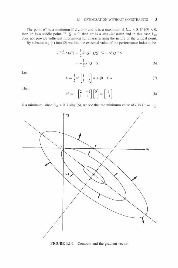
FIGURE 1.1-1 Contours and the gradient vector.

4 STATIC OPTIMIZATION

The contours of the L(u) in (7) are drawn in Fig. 1.1-1, where u = [u1 u2]T. Thearrows represent the gradient

Lu = Qu + S =[

u1 + u2

u1 + 2u2 + 1

]. (9)

Note that the gradient is always perpendicular to the contours and pointing in the directionof increasing L(u).

We shall use an asterisk to denote optimal values of u and L when we want to beexplicit. Usually, however, the asterisk will be omitted. �

Example 1.1-2. Optimization by Scalar Manipulations

We have discussed optimization in terms of vectors and the gradient. As an alternativeapproach, we could deal entirely in terms of scalar quantities. To demonstrate, let

L(u1, u2) = 1

2u21 + u1u2 + u2

2 + u2, (1)

where u1 and u2 are scalars. A critical point is present where the derivatives of L withrespect to all arguments are equal to zero:

∂L

∂u1= u1 + u2 = 0,

∂L

∂u2= u1 + 2u2 + 1 = 0. (2)

Solving this system of equations yields

u1 = 1, u2 = −1; (3)

thus, the critical point is (1, −1). Note that (1) is an expanded version of (7) inExample 1.1-1, so we have just derived the same answer by another means.

Vector notation is a tool that simplifies the bookkeeping involved in dealing withmultidimensional quantities, and for that reason it is very attractive for our purposes. �

1.2 OPTIMIZATION WITH EQUALITY CONSTRAINTS

Now let the scalar performance index be L(x , u), a function of the control vectoru ∈ Rm and an auxiliary (state) vector x ∈ Rn. The optimization problem isto determine the control vector u that minimizes L(x , u) and at the same timesatisfies the constraint equation

f (x, u) = 0. (1.2-1)

1.2 OPTIMIZATION WITH EQUALITY CONSTRAINTS 5

The auxiliary vector x is determined for a given u by the relation (1.2-1). For agiven u, (1.2-1) defines a set of n scalar equations.

To find necessary and sufficient conditions for a local minimum that alsosatisfies f (x, u) = 0, we proceed exactly as we did in the previous section, firstexpanding dL in a Taylor series and then examining the first- and second-orderterms. Let us first gain some insight into the problem, however, by consideringit from three points of view (Bryson and Ho 1975, Athans and Falb 1966).

Lagrange Multipliers and the Hamiltonian

Necessary Conditions At a stationary point, dL is equal to zero in the first-orderapproximation with respect to increments du when df is zero. Thus, at a criticalpoint the following equations are satisfied:

dL = LTu du + LT

x dx = 0 (1.2-2)

and

df = fu du + fx dx = 0. (1.2-3)

Since (1.2-1) determines x for a given u , the increment dx is determinedby (1.2-3) for a given control increment du . Thus, the Jacobian matrix fx isnonsingular and one can write

dx = −f −1x fu du. (1.2-4)

Substituting this into (1.2-2) yields

dL = (LT

u − LTxf −1

x fu

)du. (1.2-5)

The derivative of L with respect to u holding f constant is therefore given by

∂L

∂u

∣∣∣∣df=0

= (LT

u − LTxf −1

x fu

)T = Lu − f Tu f −T

x Lx, (1.2-6)

where f −Tx means (f −1

x )T. Note that

∂L

∂u

∣∣∣∣dx=0

= Lu. (1.2-7)

Thus, for dL to be zero in the first-order approximation with respect to arbitraryincrements du when df = 0, we must have

Lu − f Tu f −T

x Lx = 0. (1.2-8)

6 STATIC OPTIMIZATION

This is a necessary condition for a minimum. Before we derive a sufficientcondition, let us develop some more insight by examining two more ways toobtain (1.2-8). Write (1.2-2) and (1.2-3) as

[dL

df

]=

[LT

x LTu

fx fu

] [dx

du

]= 0. (1.2-9)

This set of linear equations defines a stationary point, and it must have a solution[dxT duT]T. The critical point is obtained only if the (n + 1) × (n + m) coefficientmatrix has rank less than n + 1. That is, its rows must be linearly dependent sothere exists an n vector λ such that

[1 λT]

[LT

x LTu

fx fu

]= 0. (1.2-10)

ThenLT

x + λTfx = 0, (1.2-11)

LTu + λTfu = 0. (1.2-12)

Solving (1.2-11) for λ gives

λT = −LTxf −1

x , (1.2-13)

and substituting in (1.2-12) again yields the condition (1.2-8) for a critical point.Note. The left-hand side of (1.2-8) is the transpose of the Schur complement

of LTu in the coefficient matrix of (1.2-9) (see Appendix A for more details).

The vector λ ∈ Rn is called a Lagrange multiplier , and it will turn out to bean extremely useful tool for us. To give it some additional meaning now, letdu = 0 in (1.2-2), (1.2-3) and eliminate dx to get

dL = LTxf −1

x df. (1.2-14)

Therefore,∂L

∂f

∣∣∣∣du=0

= (LT

xf −1x

)T = −λ, (1.2-15)

so that −λ is the partial of L with respect to the constraint holding the controlu constant. It shows the effect on the performance index of holding the controlconstant when the constraints are changed.

As a third method of obtaining (1.2-8), let us develop the approach we shall usefor our analysis in subsequent chapters. Include the constraints in the performanceindex to define the Hamiltonian function

H(x, u, λ) = L(x, u) + λTf (x, u), (1.2-16)

1.2 OPTIMIZATION WITH EQUALITY CONSTRAINTS 7

where λ ∈ Rn is an as yet undetermined Lagrange multiplier. To determine x, u ,and λ, which result in a critical point, we proceed as follows.

Increments in H depend on increments in x, u , and λ according to

dH = HTx dx + HT

u du + HTλ dλ. (1.2-17)

Note thatHλ = ∂H

∂λ= f (x, u), (1.2-18)

so suppose we choose some value of u and demand that

Hλ = 0. (1.2-19)

Then x is determined for the given u by f (x , u) = 0, which is the constraintrelation. In this situation the Hamiltonian equals the performance index:

H |f =0 = L. (1.2-20)

Recall that if f = 0, then dx is given in terms of du by (1.2-4). We should rathernot take into account this coupling between du and dx , so it is convenient tochoose λ so that

Hx = 0. (1.2-21)

Then, by (1.2-17), increments dx do not contribute to dH . Note that this yieldsa value for λ given by

∂H

∂x= Lx + f T

x λ = 0 (1.2-22)

or (1.2-13).If (1.2-19) and (1.2-21) hold, then

dL = dH = HTu du, (1.2-23)

since H = L in this situation. To achieve a stationary point, we must thereforefinally impose the stationarity condition

Hu = 0. (1.2-24)

8 STATIC OPTIMIZATION

In summary, necessary conditions for a minimum point of L(x , u) that alsosatisfies the constraint f (x , u) = 0 are

∂H

∂λ= f = 0, (1.2-25a)

∂H

∂x= Lx + f T

x λ = 0, (1.2-25b)

∂H

∂u= Lu + f T

u λ = 0, (1.2-25c)

with H (x , u , λ) defined by (1.2-16). The way we shall often use them, these threeequations serve to determine x , λ, and u in that respective order. The last two ofthese equations are (1.2-11) and (1.2-12). In most applications determining thevalue of λ is not of interest, but this value is required, since it is an intermediatevariable that allows us to determine the quantities of interest, u , x , and theminimum value of L.

The usefulness of the Lagrange-multiplier approach can be summarized asfollows. In reality dx and du are not independent increments, because of (1.2-4).By introducing an undetermined multiplier λ, however, we obtain an extra degreeof freedom, and λ can be selected to make dx and du behave as if they wereindependent increments. Therefore, setting independently to zero the gradientsof H with respect to all arguments as in (1.2-25) yields a critical point. Byintroducing Lagrange multipliers, the problem of minimizing L(x , u) subjectto the constraint f (x , u) = 0 is replaced with the problem of minimizing theHamiltonian H (x , u , λ) without constraints .

Sufficient Conditions Conditions (1.2-25) determine a stationary (critical)point. We are now ready to derive a test that guarantees that this point is aminimum. We proceed as we did in Section 1.1.

Write Taylor series expansions for increments in L and f as

dL = [LT

x LTu

] [dx

du

]+ 1

2

[dxT duT] [

Lxx Lxu

Lux Luu

] [dx

du

]+ O(3), (1.2-26)

df = [fx fu]

[dx

du

]+ 1

2

[dxT duT] [

fxx fxu

fux fuu

] [dx

du

]+ O(3), (1.2-27)

where

fxu�= ∂2f

∂u dx

and so on. (What are the dimensions of fxu?) To introduce the Hamiltonian, usethese equations to see that

[1 λT] [

dLdf

]= [

HTx HT

u

] [dx

du

]+ 1

2

[dxT duT] [

Hxx Hxu

Hux Huu

] [dx

du

]+ O(3).

(1.2-28)

1.2 OPTIMIZATION WITH EQUALITY CONSTRAINTS 9

A critical point requires that f = 0, and also that dL is zero in the first-orderapproximation for all increments dx, du . Since f is held equal to zero, df is alsozero. Thus, these conditions require Hx = 0 and Hu = 0 exactly as in (1.2-25).

To find sufficient conditions for a minimum, let us examine the second-orderterm. First, it is necessary to include in (1.2-28) the dependence of dx on du .Hence, let us suppose we are at a critical point so that Hx = 0, Hu = 0, anddf = 0. Then by (1.2-27)

dx = −f −1x fu du + O(2). (1.2-29)

Substituting this relation into (1.2-28) yields

dL = 1

2duT

[−f Tu f −T

x I] [

Hxx Hxu

Hux Huu

] [−f −1x fu

I

]du + O(3). (1.2-30)

To ensure a minimum, dL in (1.2-30) should be positive for all increments du .This is guaranteed if the curvature matrix with constant f equal to zero

Lfuu

�= Luu|f = [−f Tu f −T

x I] [

Hxx Hxu

Hux Huu

] [−f −1x fu

I

]

= Huu − f Tu f −T

x Hxu − Huxf−1x fu + f T

u f −Tx Hxxf

−1x fu (1.2-31)

is positive definite. Note that if the constraint f (x, u) is identically zero for allx and u , then (1.2-31) reduces to Luu in (1.1-6). If (1.2-31) is negative definite(indefinite), then the stationary point is a constrained maximum (saddle point).

Examples

To gain a feel for the theory we have just developed, let us consider someexamples. The first example is a geometric problem that allows easy visualization,while the second involves a quadratic performance index and linear constraint.The second example is representative of the case that is used extensively incontroller design for linear systems.

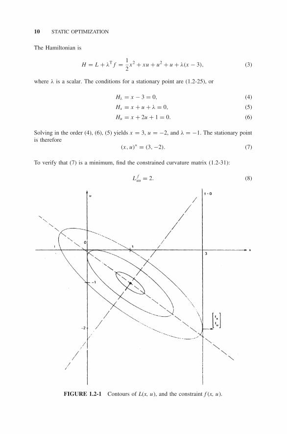
Example 1.2-1. Quadratic Surface with Linear Constraint

Suppose the performance index is as given in Example 1.1-1:

L(x, u) = 1

2[x u]

[1 11 2

] [x

u

]+ [0 1]

[x

u

], (1)

where we have simply renamed the old scalar components u1, u2 as x, u , respectively.Let the constraint be

f (x, u) = x − 3 = 0. (2)

10 STATIC OPTIMIZATION

The Hamiltonian is

H = L + λTf = 1

2x2 + xu + u2 + u + λ(x − 3), (3)

where λ is a scalar. The conditions for a stationary point are (1.2-25), or

Hλ = x − 3 = 0, (4)

Hx = x + u + λ = 0, (5)

Hu = x + 2u + 1 = 0. (6)

Solving in the order (4), (6), (5) yields x = 3, u = −2, and λ = −1. The stationary pointis therefore

(x, u)∗ = (3,−2). (7)

To verify that (7) is a minimum, find the constrained curvature matrix (1.2-31):

Lfuu = 2. (8)

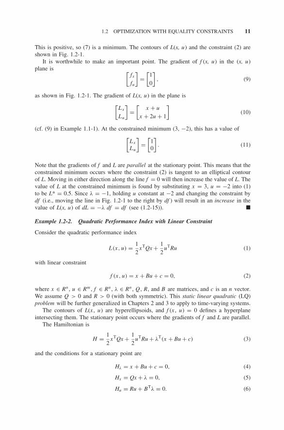
FIGURE 1.2-1 Contours of L(x, u), and the constraint f (x, u).

1.2 OPTIMIZATION WITH EQUALITY CONSTRAINTS 11

This is positive, so (7) is a minimum. The contours of L(x, u) and the constraint (2) areshown in Fig. 1.2-1.

It is worthwhile to make an important point. The gradient of f (x, u) in the (x, u)plane is [

fx

fu

]=

[1

0

], (9)

as shown in Fig. 1.2-1. The gradient of L(x, u) in the plane is[Lx

Lu

]=

[x + u

x + 2u + 1

](10)

(cf. (9) in Example 1.1-1). At the constrained minimum (3, −2), this has a value of[Lx

Lu

]=

[10

]. (11)

Note that the gradients of f and L are parallel at the stationary point. This means that theconstrained minimum occurs where the constraint (2) is tangent to an elliptical contourof L. Moving in either direction along the line f = 0 will then increase the value of L. Thevalue of L at the constrained minimum is found by substituting x = 3, u = −2 into (1)to be L* = 0.5. Since λ = −1, holding u constant at −2 and changing the constraint bydf (i.e., moving the line in Fig. 1.2-1 to the right by df ) will result in an increase in thevalue of L(x, u) of dL = −λ df = df (see (1.2-15)). �

Example 1.2-2. Quadratic Performance Index with Linear Constraint

Consider the quadratic performance index

L(x, u) = 1

2xTQx + 1

2uTRu (1)

with linear constraint

f (x, u) = x + Bu + c = 0, (2)

where x ∈ Rn , u ∈ Rm , f ∈ Rn , λ ∈ Rn , Q , R, and B are matrices, and c is an n vector.We assume Q > 0 and R > 0 (with both symmetric). This static linear quadratic (LQ)problem will be further generalized in Chapters 2 and 3 to apply to time-varying systems.

The contours of L(x , u) are hyperellipsoids, and f (x , u) = 0 defines a hyperplaneintersecting them. The stationary point occurs where the gradients of f and L are parallel.

The Hamiltonian is

H = 1

2xTQx + 1

2uTRu + λT(x + Bu + c) (3)

and the conditions for a stationary point are

Hλ = x + Bu + c = 0, (4)

Hx = Qx + λ = 0, (5)

Hu = Ru + BTλ = 0. (6)

12 STATIC OPTIMIZATION

To solve these, first use the stationarity condition (6) to find an expression for u in termsof λ,

u = −R−1BTλ. (7)

According to (5)λ = −Qx, (8)

and taking into account (4) results in

λ = QBu + Qc. (9)

Using this in (7) yields

u = −R−1BT(QBu + Qc) (10)

or(I + R−1BTQB)u = −R−1BTQc,

(R + BTQB)u = −BTQc. (11)

Since R > 0 and BTQB > 0, we can invert R + BTQB and so the optimal control is

u = −(R + BTQB)−1BTQc. (12)

Using (12) in (4) and (9) gives the optimal-state and multiplier values of

x = −(I − B(R + BTQB)−1BTQ)c, (13)

λ = (Q − QB(R + BTQB)−1BTQ)c. (14)

By the matrix inversion lemma (see Appendix A)

λ = (Q−1 + BR−1BT)−1c (15)

if |Q| �= 0.To verify that control (12) results in a minimum, use (1.2-31) to determine that the

constrained curvature matrix is

Lfuu = R + BTQB, (16)

which is positive definite by our restrictions on R and Q . Using (12) and (13) in (1) yieldsthe optimal value

L∗ = 1

2cT

[Q − QB(R + BTQB)−1BTQ

]c, (17)

L∗ = 1

2cTλ, (18)

so that∂L∗

∂c= λ. (19)

�

1.2 OPTIMIZATION WITH EQUALITY CONSTRAINTS 13

Effect of Changes in Constraints

Equation (1.2-28) expresses the increment dL in terms of df, dx , and du . In thediscussion following that equation we let df = 0, found dx in terms of du ,and expressed dL in terms of du . That gave us conditions for a stationary point(Hx = 0 and Hu = 0) and led to the second-order coefficient matrix L

fuu in

(1.2-31), which provided a test for the stationary point to be a constrainedminimum.

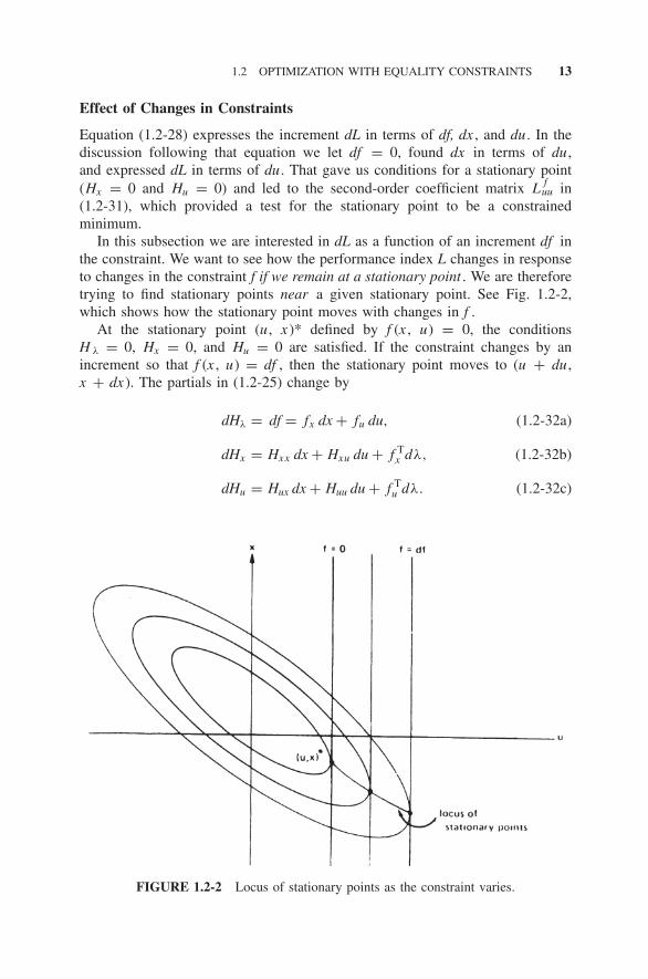
In this subsection we are interested in dL as a function of an increment df inthe constraint. We want to see how the performance index L changes in responseto changes in the constraint f if we remain at a stationary point . We are thereforetrying to find stationary points near a given stationary point. See Fig. 1.2-2,which shows how the stationary point moves with changes in f .

At the stationary point (u , x )* defined by f (x , u) = 0, the conditionsH λ = 0, Hx = 0, and Hu = 0 are satisfied. If the constraint changes by anincrement so that f (x , u) = df , then the stationary point moves to (u + du ,x + dx ). The partials in (1.2-25) change by

dHλ = df = fx dx + fu du, (1.2-32a)

dHx = Hxx dx + Hxu du + f Tx dλ, (1.2-32b)

dHu = Hux dx + Huu du + f Tu dλ. (1.2-32c)

FIGURE 1.2-2 Locus of stationary points as the constraint varies.

14 STATIC OPTIMIZATION

In order that we remain at a stationary point, the increments dHx and dHu

should be zero. This requirement imposes certain relations between the changesdx, du , and df , which we shall use in (1.2-28) to determine dL as a functionof df .

To find dx and du as functions of df with the requirement that we remain atan optimal solution, use (1.2-32a) to find

dx = f −1x df − f −1

x fu du, (1.2-33)

and set (1.2-32b) to zero to find

dλ = −f −Tx (Hxx dx + Hxu du). (1.2-34)

Now use these relations in (1.2-32c) to obtain

dHu = (Huu − Huxf

−1x fu − f T

u f −Tx Hxu + f T

u f −Tx Hxxf

−1x fu

)du

+ (Hux − f T

u f −Tx Hxx

)f −1

x df = 0

so that

du = − (Lfuu

)−1 (Hux − f T

u f −Tx Hxx

)f −1

x df�= −C df. (1.2-35)

Using (1.2-35) in (1.2-33) yields

dx =[I + f −1

x fu

(Lfuu

)−1 (Hux − f T

u f −1x Hxx

)]f −1

x df

= f −1x (I + fuC) df. (1.2-36)

Equations (1.2-35) and (1.2-36) are the required expressions for the incrementsin the stationary values of control and state as functions of df . If |Lf

uu| �= 0, thendx and du can be determined in terms of df , and the existence of neighboringoptimal solutions as f varies is guaranteed.

To determine the increment dL in the optimal performance index as a functionof df , substitute (1.2-35) and (1.2-36) into (1.2-28), using Hx = 0, dHu = 0,since we began at a stationary point (u , x )*. The result is found after some workto be

dL = −λT df + 1

2dfT

(f −T

x Hxxf−1x − CTLf

uuC)df + O(3). (1.2-37)

From this we see that the first and second partial derivatives of L*(x , u) withrespect to f (x, u) under the restrictions dHx = 0, dHu = 0 are

∂L∗

∂f

∣∣∣∣Hx,Hu

= −λ, (1.2-38)

∂2L∗

∂f 2

∣∣∣∣Hx,Hu

= f −Tx Hxxf

−1x − CTLf

uuC. (1.2-39)

PROBLEMS 15

Equation (1.2-38) allows a further interpretation of the Lagrange multiplier; itindicates the rate of change of the optimal value of the performance index withrespect to the constraint.

1.3 NUMERICAL SOLUTION METHODS

Analytic solutions for the stationary point (u , x )* and minimal value L* ofthe performance index cannot be found except for simple functions L(x, u) andf (x, u). In most practical cases, numerical optimization methods must be used.Many methods exist, but steepest descent or gradient (Luenberger 1969, Brysonand Ho 1975) methods are probably the simplest.

The steps in constrained minimization by the method of steepest descent are(Bryson and Ho 1975)

1. Select an initial value for u .2. Determine x from f (x , u) = 0.3. Determine λ from λ = −f −T

x Lx .4. Determine the gradient vector Hu = Lu + f T

u λ.5. Update the control vector by �u = −αHu, where K is a positive scalar

constant (to find a maximum use �u = αHu).6. Determine the predicted change in the value of L, �L = HT

u �u =−αHT

u Hu. If �L is sufficiently small, stop. Otherwise, go to step 2.

There are many variations to this procedure. If the step-size constant K is toolarge, then the algorithm may overshoot the stationary point (u , x )* and con-vergence may not occur. The step size should usually be reduced as (u , x )*is approached, and several of the existing variations differ in the approach toadapting K .

Many software routines are available for unconstrained optimization. Thenumerical solution of the constrained optimization problem of minimizingL(x, u) subject to f (x , u) = 0 can be obtained using the MATLAB functionconstr.m available under the Optimization Toolbox. This function takes in theuser-defined subroutine funct.m , which computes the value of the function, theconstraints, and the initial conditions.

PROBLEMS

Section 1.1

1.1-1. Find the critical points u* (classify them) and the value of L(u*) inExample 1.1-1 if

a. Q =[−1 11 −2

], ST = [0 1].

16 STATIC OPTIMIZATION

b. Q =[−1 11 2

], ST = [0 1].

Sketch the contours of L and find the gradient Lu.

1.1-2. Find the minimum value of

L(x1, x2) = x21 − x1x2 + x2

2 + 3x1. (1)

Find the curvature matrix at the minimum. Sketch the contours, showing thegradient at several points.

1.1-3. Failure of test for minimality. The function f (x, y) = x2 + y4 has aminimum at the origin.a. Verify that the origin is a critical point.b. Show that the curvature matrix is singular at the origin.c. Prove that the critical point is indeed a minimum.

Section 1.2

1.2-1. Ship closest point of approach. A ship is moving at 10 miles per houron a course of 30◦ (measured clockwise from north, which is 0◦). Find its closestpoint of approach to an island that at time t = 0 is 20 miles east and 30 milesnorth of it. Find the distance to the island at this point. Find the time of closestapproach.

1.2-2. Shortest distance between two points. Let P1 = (x1, y1) and P2 =(x2, y2) be two given points. Find the third point P3 = (x3, y3) such thatd1 = d2 is minimized, where d1 is the distance from P3 to P1 and d2 is thedistance from P3 to P2.

1.2-3. Meteor closest point of approach. A meteor is in a hyperbolic orbitdescribed with respect to the earth at the origin by

x2

a2− y2

b2= 1. (1)

Find its closest point of approach to a satellite that is in such an orbit that it hasa constant position of (x1, y1). Verify that the solution indeed yields a minimum.

1.2-4. Shortest distance between a parabola and a point. A meteor is movingalong the path

y = x2 + 3x − 6. (1)

A space station is at the point (x , y) = (2, 2).a. Use Lagrange multipliers to find a cubic equation for x at the closest point of

approach.