optimal combination forecasts for hierarchical time...

ISSN 1440-771X

Department of Econometrics and Business Statistics

http://www.buseco.monash.edu.au/depts/ebs/pubs/wpapers/

Optimal combination forecasts

for hierarchical time series

Rob J Hyndman, Roman A Ahmed and

George Athanasopoulos

July 2007

Working Paper 09/07

Optimal combination forecasts for

hierarchical time series

Rob J Hyndman

Department of Econometrics and Business Statistics,

Monash University, VIC 3800, Australia.

Email: [email protected]

Roman A Ahmed




George Athanasopoulos




17 July 2007

JEL classification: C53,C32,C23

Optimal combination forecasts for

hierarchical time series

Abstract: In many applications, there are multiple time series that are hierarchically organized

and can be aggregated at several different levels in groups based on products, geography or

some other features. We call these “hierarchical time series”. They are commonly forecast using

either a “bottom-up” or a “top-down” method.

In this paper we propose a new approach to hierarchical forecasting which provides optimal

forecasts that are better than forecasts produced by either a top-down or a bottom-up approach.

Our method is based on independently forecasting all series at all levels of the hierarchy and

then using a regression model to optimally combine and reconcile these forecasts. The resulting

revised forecasts add up appropriately across the hierarchy, are unbiased and have minimum

variance amongst all combination forecasts under some simple assumptions.

We show in a simulation study that our method performs well compared to the top-down approach

and the bottom-up method. It also allows us to construct prediction intervals for the resultant

forecasts.

Finally, we apply the method to forecasting Australian tourism demand where the data are disag-

gregated by purpose of visit and geographical region.

Keywords: bottom-up forecasting, combining forecasts, GLS regression, hierarchical forecast-

ing, Moore-Penrose inverse, reconciling forecasts, top-down forecasting.

Optimal combination forecasts for hierarchical time series

1 Introduction

In business and economics there are often applications requiring forecasts of many related time

series organized in a hierarchical structure based on dimensions such as product and geography.

This has led to the need for reconciling forecasts across the hierarchy (that is, ensuring the

forecasts sum appropriately across the levels).

We propose a new statistical method for forecasting hierarchical time series which (1) provides

point forecasts that are reconciled across the levels of hierarchy; (2) allows for the correlations

and interaction between the series at each level of the hierarchy; (3) provides estimates of fore-

cast uncertainty which are reconciled across the levels of hierarchy; and (4) is sufficiently flexible

that ad hoc adjustments can be incorporated, information about individual series can be allowed

for, and important covariates can be included. Furthermore, our method provides optimal fore-

casts under some simple assumptions.

This problem arises in many different contexts. For example, forecasting manufacturing demand

typically involves a hierarchy of time series. One of us has worked for a disposable tableware

manufacturer who wanted forecasts of all paper plates, of each different type of paper plate, and

of each type of plate at each distribution outlet. Another of us has been involved in forecasting

net labour turnover. Not only is it important to forecast the rate of job turnover in the economy as

a whole and across major occupational groups, but it is also important to do so at the individual

occupation level. The hierarchical structure according to the Australian Standard Classification

of Occupations (ASCO), starting from the highest level, can be illustrated as follows:

• All employed persons

– Professionals (major group)

Educational professionals (sub-major group)

· School teachers (minor group)

* Pre-primary teachers (unit group)

* Primary teachers (unit group); etc.

There are 340 unit groups in ASCO. Further divisions of the unit groups can be made by gender

and age variables. The series at the lowest level can be short in length with a high degree

of volatility but aggregate behavior may be relatively smooth. Thus the problem here is that

of forecasting a set of time series that are hierarchical in structure and clusters of which may

be correlated. In Section 2, we introduce some notation to allow the problem of hierarchical

2


forecasting to be defined more precisely.

The various components of the hierarchy can interact in varying and complex ways. A change in

one series at one level, can have a consequential impact on other series at the same level, as well

as series at higher and lower levels. Current forecasting methodology for hierarchical systems

has not attempted to model this complex behavior at all. By modeling the entire hierarchy of time

series simultaneously, we will obtain better forecasts of the component series.

Existing approaches to hierarchical forecasting usually involve either a top-down or bottom-up

method, or a combination of the two. The top-down method entails forecasting the completely

aggregated series, and then disaggregating the forecasts based on historical proportions. Gross

and Sohl (1990) discuss several possible ways of choosing these proportions. The bottom-up

method involves forecasting each of the disaggregated series at the lowest level of the hierarchy,

and then using simple aggregation to obtain forecasts at higher levels of the hierarchy. In prac-

tice, many businesses combine these methods (giving what is sometimes called the “middle-out”

method) where forecasts are obtained for each series at an intermediate level of the hierarchy,

and then aggregation is used to obtain forecasts at higher levels and disaggregation is used to

obtain forecasts at lower levels.

Of course, it is also possible to forecast all series at all levels independently, but this has the

undesirable consequence of the higher level forecasts not being equal to the sum of the lower

level forecasts. Consequently, if this method is used, some adjustment is then carried out to

ensure the forecasts add up appropriately. These adjustments are usually done in an ad hoc

manner.

None of these methods take account of the inherent correlation structure of the hierarchy, and it

is not easy to obtain prediction intervals for the forecasts from any of these methods.

We present a framework for general hierarchical forecasting in Section 3, and show that existing

methods are special cases of this framework. We also show how to obtain prediction intervals for

any of the methods that are special cases of our framework.

Most of the forecasting literature in this area has looked at the comparative performance of the

top-down and bottom-up methods. An early contribution was Grunfeld and Griliches (1960) who

argued that the disaggregated data are error-prone and that top-down forecasts may therefore

be more accurate. Similar conclusions were drawn by Fogarty et al. (1990) and Narasimhan

et al. (1994). Fliedner (1999) also argued that aggregate forecast performance is better with

3


aggregate level data. On the other hand, Orcutt et al. (1968) and Edwards and Orcutt (1969)

argued that information loss is substantial in aggregation and therefore the bottom-up method

gives more accurate forecasts. Shlifer and Wolff (1979) compared the forecasting performance

of both methods and concluded that the bottom-up method is preferable under some conditions

on the structure of the hierarchy and the forecast horizon. Schwarzkopf et al. (1988) looked at

the bias and robustness of the two methods and concluded that the bottom-up method is better

except when there are missing or unreliable data at the lowest levels.

Empirical studies have supported the efficacy of bottom-up forecasting over top-down forecast-

ing. For example, Kinney (1971) found that disaggregated earnings data by market segments

resulted in more accurate forecasts than when firm-level data were used. Collins (1976) com-

pared segmented econometric models with aggregate models for a group of 96 firms, and found

the segmented models produced more accurate forecasts for both sales and profit. The study

of telephone demand by Dunn et al. (1976) shows that forecasts aggregated from lower-level

modeling are more accurate than the top-down method. Zellner and Tobias (2000) used annual

GDP growth rates from 18 countries and found that disaggregation provided better forecasts.

Dangerfield and Morris (1992) constructed artificial 2-level hierarchies using the M-competition

data with two series at the bottom level, and found that bottom-up forecasts were more accurate,

especially when the two bottom-level series were highly correlated.

Tiao and Guttman (1980) and Kohn (1982) used more theoretical arguments to show that the effi-

ciency of aggregation depends on the covariance structure of the component series. Shing (1993)

discussed some time series models and demonstrated that there is no uniform superiority of one

method over the other. Fliedner and Lawrence (1995) concluded that current formal hierarchical

forecasting techniques have no advantage over some informal strategies of hierarchical forecast-

ing. Kahn (1998) suggested that it is time to combine the existing methodologies so that we can

enjoy the good features of both methods, but no specific ideas were provided in that discussion.

Another very good discussion paper is Fliedner (2001) who summarizes the uses and application

guidelines for hierarchical forecasting. However, none of these papers provide any new methods

and none discuss the construction of prediction intervals for hierarchical forecasts.

In Section 4, we take up the call of Kahn (1998) by proposing a new methodology which takes the

best features of existing methods, and provides a sound statistical basis for optimal hierarchical

forecasting. We discuss computational issues associated with our method in Section 5.

The performance of our optimal hierarchical forecasts is evaluated using a simulation exercise in

4


Section 6, where we compare our method with the major existing methods. Then, in Section 7, we

apply the various methods to some real data, Australian domestic tourism demand, disaggregated

by geographical region and by purpose of travel. In both the simulations and the real data

application, we find that our method produces, on average, more accurate forecasts than existing

approaches.

We conclude the paper by summarizing our findings and suggesting some possible extensions in

Section 8.

2 Notation for hierarchical forecasting

Consider a multi-level hierarchy where level 0 denotes the completely aggregated series, level 1

the first level of disaggregation, down to level K containing the most disaggregated time series.

We use a sequence of letters to identify the individual series and the level of disaggregation. For

example: A denotes series A at level 1; AF denotes series F at level 2 within series A at level 1;

AFC denotes series C at level 3 within series AF at level 2; and so on.

To be specific, suppose we had three levels in the hierarchy with each group at each level con-

sisting of three series. In this case, K = 3 and the hierarchy has the tree structure shown in

Figure 1.

Figure 1: A three level hierarchical tree diagram.

Total

A

AA

AAA AAB AAC

AB

ABA ABB ABC

AC

ACA ACB ACC

B

BA

BAA BAB BAC

BB

BBA BBB BBC

BC

BCA BCB BCC

C

CA

CAA CAB CAC

CB

CBA CBB CBC

CC

CCA CCB CCC

It is assumed that observations are recorded at times t = 1,2, . . . , n, and that we are interested

in forecasting each series at each level at times t = n+ 1, n+ 2, . . . , n+ h. It will sometimes be

convenient to use the notation X to refer to a generic series within the hierarchy. Observations

on series X are written as YX,t . Thus, YAF,t is the value at time t on series AF. We use Yt for the

5


aggregate of all series at time t. Therefore

Yt =∑

i

Yi,t , Yi,t =∑

j

Yi j,t , Yi j,t =∑

k

Yi jk,t , Yi jk,t =∑

ℓ

Yi jkℓ,t ,

and so on. Thus, observations at higher levels can be obtained by summing the series below.

Let mi denote the total number of series at level i, i = 0,1,2, . . . , K . So mi > mi−1 and the total

number of series in the hierarchy is m= m0+m1+m2+ · · ·+mK . In the example above, mi = 3i

and m= 40.

It will be convenient to work with matrix and vector expressions. We let Yi,t denote the vector of

all observations at level i and time t and Yt =

Yt , Y1,t , . . . , YK,t

′. Note that

Yt = SYK,t (1)

where S is a “summing” matrix of order m×mK used to aggregate the lowest level series.

In the above example,

Yt =

Yt , YA,t , YB,t , YC,t , YAA,t , YAB,t , . . . , YCC,t , YAAA,t , YAAB,t , . . . , YCCC,t

′

and the summation matrix is of order 40× 27 and is given by

S =

111111111111111111111111111

111111111000000000000000000

000000000111111111000000000

000000000000000000111111111

111000000000000000000000000

000011100000000000000000000

...

000000000000000000000000111

100000000000000000000000000

010000000000000000000000000

...

000000000000000000000000001

.

6


The rank of S is mK . It is clear that the S matrix can be partitioned by the levels of the hierarchy.

The top row is a unit vector of length mK and the bottom section is an mK ×mK identity matrix.

The middle parts of S are vector diagonal rectangular matrices.

While aggregation is our main interest here, the results to follow are sufficiently general that S

can be a general linear operator, and need not be restricted to aggregation.

3 General hierarchical forecasting

Suppose we first compute forecasts for each series at each level giving m base forecasts for each

of the periods n + 1, . . . , n + h, based on the information available up to and including time n.

We denote these base forecasts by YX,n(h) where X denotes the series being forecasted. Thus,

Yn(h) denotes the h-step-ahead base forecast of the total, YA,n(h) denotes the forecast of series

A, YAC,n(h) denotes the forecast of series AC, and so on. We let Yn(h) be the vector consisting of

these base forecasts, stacked in the same series order as for Yt .

All existing hierarchical forecasting methods can then be written as

Yn(h) = SPYn(h) (2)

for some appropriately chosen matrix P of order mK ×m. That is, existing methods involve linear

combinations of the base forecasts. These linear combinations are “reconciled” in the sense that

lower level forecasts sum to give higher level forecasts. The effect of the P matrix is to extract

and combine the relevant elements of the base forecasts Yn(h) which are then summed by S to

give the final revised hierarchical forecasts, Yn(h).

For example, bottom-up forecasts are obtained using

P =

0mK×(m−mK )| ImK

, (3)

where 0ℓ×k is a null matrix of order ℓ× k and Ik is an identity matrix of order k× k. In this case,

the P matrix extracts only bottom-level forecasts from Yn(h) which are then summed by S to give

the bottom-up forecasts.

7


Top-down forecasts are obtained using

P =

p | 0mK×(m−1)

(4)

where p = [p1, p2, . . . , pmK]′ is a vector of proportions that sum to one. The effect of the P matrix

here is to distribute the forecast of the aggregate to the lowest level series. Different methods of

top-down forecasting lead to different proportionality vectors p.

Variations such as middle-out forecasts are possible by defining the matrix P appropriately. This

suggests that other (new) hierarchical forecasting methods may be defined by choosing a differ-

ent matrix P provided we place some restrictions on P to give sensible forecasts.

If we assume that the base (independent) forecasts are unbiased (that is, E[Yn(h)] = E[Yn(h)]),

and that we want the revised hierarchical forecasts to also be unbiased, then we must require

E[Yn(h)] = E[Yn(h)] = SE[YK,n(h)]. Suppose βn(h) = E[YK,n+h | Y1, . . . , Yn] is the mean of the fu-

ture values of the bottom level K . Then E[Yn(h)] = SPE[Yn(h)] = SPSβn(h). So, the unbiasedness

of the revised forecast will hold provided

SPS = S. (5)

This condition is true for the bottom-up method with P given by (3). However, using the top-down

method with P given by (4), we find that SPS 6= S for any choice of p. So the top-down method

can never give unbiased forecasts even if the base forecasts are unbiased.

Let the variance of the base forecasts, Yn(h), be given by Σh. Then the variance of the revised

forecasts is given by

Var[Yn(h)] = SPΣhP ′S′. (6)

Thus, prediction intervals on the revised forecasts can be obtained provided Σh can be reliably

estimated. Note that result (6) applies to all the existing methods that can be expressed as (2)

including bottom-up, top-down and middle-out methods.

8


4 Optimal forecasts using regression

We can write the base forecasts as

Yn(h) = Sβn(h) + ǫh (7)

where βn(h) = E[YK,n+h | Y1, . . . , Yn] is the unknown mean of the bottom level K , and ǫh has zero

mean and covariance matrix Var(ǫh) = Σh. This suggests that we can estimate βn(h) by treating

(7) as a regression equation, and thereby obtain forecasts for all levels of the hierarchy. If Σh

was known, we could use generalized least squares estimation to obtain the minimum variance

unbiased estimate of βn(h) as

βn(h) = (S′Σ

†

hS)−1S′Σ

†

hYn(h) (8)

where Σ†

his the Moore-Penrose generalized inverse of Σh. We use a generalized inverse because

Σh is often (near) singular due to the aggregation involved in Yn. This leads to the following

revised forecasts

Yn(h) = Sβn(h) = SPYn(h)

where P = (S′Σ†

hS)−1S′Σ

†

h. Clearly this satisfies the unbiasedness property (5). The variance of

these forecasts is given by

Var[Yn(h)] = S(S′Σ†

hS)−1S′.

The difficulty with this method is that it requires knowledge of Σh, or at least a good estimate of

it. In a large hierarchy, with thousands of series, this may not be possible.

However, we can greatly simplify the computations by expressing the error in (7) as ǫh ≈ SǫK,h

where ǫK,h is the forecast error in the bottom level. The result is not exact because the lower

level base forecasts do not necessarily add to give the upper level base forecasts. Nevertheless,

the approximation leads to the result Σh ≈ SΩhS′, where Ωh = Var(ǫK,h). We are now ready to

state our main result.

Theorem 1 Let Y = Sβh + ǫ with Var(ǫ) = Σh = SΩhS′ and S a “summing” matrix. Then the

generalized least squares estimate of β obtained using the Moore-Penrose generalized inverse is

independent of Ωh:

βh = (S′Σ

†

hS)−1S′Σ

†

hY = (S′S)−1S′Y

with variance matrix Var(β) = Ωh. Moreover, this is the minimum variance linear unbiased

9


estimate.

Proof: We write Σh = BC where B = SΩh and C = S′. Then, by Fact 6.4.8 of Bernstein (2005,

p.235), the Moore-Penrose generalized inverse of Σh is

Σ†

h= C ′(CC ′)−1(B′B)−1B′ = S(S′S)−1(Ω′

hS′SΩh)

−1Ω′hS′ . (9)

Then (S′Σ†

hS)−1S′Σ

†

h= (S′S)−1S′. The variance is obtained by substituting (9) into (S′Σ

†

hS)−1.

Tian and Wiens (2006, Theorem 3) show that the GLS estimator will be the minimum variance

unbiased estimator if and only if

SS†Σ

†

hΣh(I − SS†) = 0,

where S† = (S′S)−1S′. Using (9), it is easy to show that this condition holds.

This remarkable result shows that we can use OLS rather than GLS when computing our revised

forecasts, without the need for an estimate of the underlying covariance matrix. Thus we use

Yn(h) = S(S′S)−1S′Yn(h); (10)

in other words, P = (S′S)−1S′. The variance covariance matrix of the revised forecasts is

Var[Yn(h)] = Σh. Therefore, prediction intervals still require estimation of Σh. We leave the

discussion of strategies for estimating this matrix to a later paper.

Equation (10) shows that, under the assumption Σh = SΩhS′, the optimal combination of base

forecasts is independent of the data. For a simple hierarchy with only one level of disaggregation

(K = 1) and with m1 nodes at level 1, the weights are given by

SP = (m1 + 1)−1

m1 1 1 . . . . . . 1

1 m1 −1 −1 . . . −1

1 −1 m1 −1 −1

......

. . .. . .

. . ....

1 −1 −1. . . −1

1 −1 −1 . . . −1 m1

.

10


5 Computational pitfalls and remedies

The primary difficulty in implementing the forecasting method given by (10) is that the matrix

S can be very large, and so the computational effort required to find the inverse of S′S can be

prohibitive. Even the construction of the S matrix can be difficult for large hierarchies. We

discuss three solutions to this problem.

First, of the mK m elements in the S matrix, there are only mK K non-zero elements. Since K

is usually much smaller than m, S is a sparse matrix. We can use sparse matrix storage and

arithmetic (e.g., Duff et al., 2002) to save computer memory and computational time. Then we

can use the algorithm of Ng and Peyton (1993) as implemented in Koenker and Ng (2007) to solve

(10). This works well for moderately large hierarchies, but for some of the large hierarchies we

encounter in practise, even this method is unsuitable.

For very large hierarchies, an iterative approach can be used based on the method of Lanczos

(1950, 1952). This method was primarily developed for solving a system of linear equations but

was subsequently extended by Golub and Kahan (1965) to work with least squares problems with

lower bidiagonalization of the coefficient matrix. Based on these methods, Paige and Saunders

(1982) developed an iterative algorithm for solving sparse linear least squares problems. Due to

the iteration process, the results are an approximation to the direct solution, but in almost all

cases in which we have used the method, the difference is negligible.

The third approach relies on a reparameterization of the regression model (7). Rather than

each parameter representing a bottom level series, we use a parameter for every series in the

hierarchy, but use some zero-sum constraints to avoid overparameterization. The new parameter

vector is denoted by φn(h) and has elements in the same order as Yt . Each parameter measures

the contribution of the associated level to the bottom level series below it. In the example shown

in Figure 1,

φn(h) =

µT,h,µA,h,µB,h,µC,h,µAA,h,µAB,h, . . . ,µCC,h,µAAA,h,µAAB,h, . . . ,µCCC,h

′,

and βAAB,h = µT,h+µA,h+µAA,h+µAAB,h. Similarly, other β values are constructed by summing the

aggregate nodes that contribute to that bottom level node. Then we can write βn(h) = S′φn(h)

so that

Yn(h) = SS′φn(h) + ǫh. (11)

11


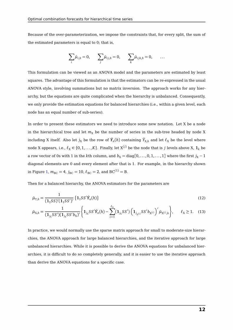
Because of the over-parameterization, we impose the constraints that, for every split, the sum of

the estimated parameters is equal to 0; that is,

∑

i

µi,h = 0,∑

j

µi j,h = 0,∑

k

µi jk,h = 0, . . .

This formulation can be viewed as an ANOVA model and the parameters are estimated by least

squares. The advantage of this formulation is that the estimators can be re-expressed in the usual

ANOVA style, involving summations but no matrix inversion. The approach works for any hier-

archy, but the equations are quite complicated when the hierarchy is unbalanced. Consequently,

we only provide the estimation equations for balanced hierarchies (i.e., within a given level, each

node has an equal number of sub-series).

In order to present these estimators we need to introduce some new notation. Let X be a node

in the hierarchical tree and let mX be the number of series in the sub-tree headed by node X

including X itself. Also let jX be the row of Yn(h) containing YX,h and let ℓX be the level where

node X appears, i.e., ℓX ∈ 0,1, . . . , K. Finally, let X( j) be the node that is j levels above X, 1k be

a row vector of 0s with 1 in the kth column, and bX = diag[0, . . . , 0,1, . . . , 1] where the first jX− 1

diagonal elements are 0 and every element after that is 1. For example, in the hierarchy shown

in Figure 1, mBC = 4, jBC = 10, ℓBC = 2, and BC(1) = B.

Then for a balanced hierarchy, the ANOVA estimators for the parameters are

µT,h =1

(11SS)′(11SS′)′

11SS′Yn(h)

(12)

µX,h =1

(1 jXSS′)(1 jX

SS′bX)′

¨

1 jXSS′Yn(h)−

ℓX∑

i=1

(1 jXSS′)

1 jX(i)

SS′bX(i)′

µX(i),h

«

, ℓX ≥ 1. (13)

In practice, we would normally use the sparse matrix approach for small to moderate-size hierar-

chies, the ANOVA approach for large balanced hierarchies, and the iterative approach for large

unbalanced hierarchies. While it is possible to derive the ANOVA equations for unbalanced hier-

archies, it is difficult to do so completely generally, and it is easier to use the iterative approach

than derive the ANOVA equations for a specific case.

12


6 Numerical simulations

In order to evaluate the performance of our proposed methodology, we first perform a simulation

study. We consider a hierarchy with K = 3 levels and m = 85 series in total. The completely

aggregated series at the top level is disaggregated into four component series at level 1, i.e.,

m1 = 4. Each of these series are further subdivided into four series at level 2, i.e., m2 = 16.

Finally, each one of the level 2 series are further disaggregated to four component series giving

a total of m3 = 64 series at the completely disaggregated bottom level.

The data for each series were generated by an ARIMA(p, d ,q) process with d taking values 1 or

2 with equal probability, and p and q each taking values 0, 1 and 2 with equal probability. For

each generated series, the parameters of each process were chosen randomly based on a uniform

distribution over the stationary and invertible regions. (However, the order and parameters of

each ARIMA process did not change across replications.)

In order to ensure the data are reconciled across the hierarchy, at each node we only generated

the aggregated data and three of its four component series. The remaining fourth component

series was generated by subtraction. Hence we generated 64 series independently (1 at the

completely aggregate level, 3 at level 1, 12 at level 2 and 48 at level 3), and the remaining 21 (1

at level 1, 4 at level 2 and 16 at level 3) are obtained by subtraction.

A typical feature of observed hierarchical time series is that, due to aggregation, the higher level

series are smoother than series at lower levels. To ensure this characteristic is replicated in

our simulated hierarchies, we set the error variance of the generated level-k series to σ2kwhere

σ20= 2 and σ2

k= 5 for k ≥ 1.

For each series we generate 100 observations. We divide the data into two parts: the first 90

observations of each series is used as a training set and the last 10 observations as a test set.

Applying the statistical framework for exponential smoothing methods developed by Hyndman

et al. (2002), we fit a state space model to the training data and obtain independent base forecasts

for each of the 85 series for 1–10 steps ahead. We prefer to use exponential smoothing models

rather than ARIMA models for forecasting as they are much faster to implement and there are

thousands of series to forecast. Also, exponential smoothing methods have been shown to give

better forecasts than ARIMA models (Makridakis and Hibon, 2000), even when the underlying

series come from ARIMA models with no equivalent exponential smoothing state space model

(Hyndman, 2001).

13


Table 1: Average MAE by level. The p-values are from a one-way ANOVA testing the differences

between methods for each level.

Level Top-down Bottom-up Combined p-value

0 (Top) 94.11 188.46 95.14 < 0.001

1 2423.33 99.11 55.49 < 0.001

2 2752.20 71.03 54.62 < 0.001

3 (Bottom) 4636.67 70.28 70.97 < 0.001

Total 9906.30 428.89 276.22

Final forecasts are produced using three different methods: (i) optimally combining the base

forecasts as advocated in Section 4; (ii) using the conventional bottom-up method, i.e., aggre-

gating the bottom level independent forecasts all the way to the top level; and (iii) applying the

conventional top-down approach where the historical proportions of the data are used to disag-

gregate the top level forecasts all the way down to the bottom level. This process was repeated

600 times.

The forecast performance of each method is now compared. In Table 1 we present the average

mean absolute error (MAE) across each level over the 600 simulated hierarchical time series. As

expected, the top-down method performs best at the top level and the bottom-up method performs

best at the bottom level. Evaluating the performance of our optimal combination method at these

extreme levels, we find that the quality of our forecasts are very similar to the best performing

method at each level. At the top level our method yields an average MAE of 95.14 in comparison

to 94.11 yielded by the best performing top-down method. We find a similar small difference at

the bottom level between our method and the best performing bottom-up method. However, our

method clearly outperforms the conventional methods at their least favourable extreme levels.

At the top level the average MAE for the optimal combination method is approximately half the

size of the bottom-up method. At the bottom level the average MAE of the top-down method is

more than 65 times that of our proposed method.

Furthermore, our proposed method clearly outperforms both conventional approaches at the

intermediate levels 1 and 2. In order to summarize the overall performance of the alternative

approaches, in the last row of Table 1 we present the total MAE yielded by each method across

all levels of the hierarchy. The consistently good performance of our optimal combination method

in comparison to the conventional approaches is reflected in this total MAEmeasure. The popular

bottom-up approach yields more than 1.5 times the total MAE of our combined method, and the

top-down method yields more than 30 times the MAE of our method.

14


Table 2: P-values for Tukey’s Honest Significant Difference test between the combination

method and other methods for each level.

Level Top-down HP Bottom-up

0 0.997 0.000

1 0.000 0.996

2 0.000 1.000

3 0.000 1.000

To formally test whether the forecasting performance of the alternative methods is different

across each level we perform a one-way analysis of variance (ANOVA). The output is summarized

in the right hand column of Table 1. The F statistic for each level follows an F3,2396 distribution.

The results uniformly show that for each and every level the null hypothesis that the alternative

methods produce similar forecasts, is rejected. Hence, there is sufficient evidence to conclude

that the forecasting performances of the alternative hierarchical methods are significantly differ-

ent at all levels.

In Table 2 we present the results from Tukey’s Honest Significant Difference (HSD) test. The

HSD test complements the ANOVA by allowing for a pairwise comparison between the alterna-

tive methods at each level. The results show that at the top-level we cannot reject the null of an

equal forecasting performance between the conventional top-down method and our combination

approach. However, we strongly reject the null hypothesis of equal MAE values when comparing

our optimal combination approach to the bottom-up approach. For levels 1, 2 and 3 there is a sta-

tistically significant difference between the forecasting performance of our optimal combination

approach and the top-down approach but no significant difference between our approach and the

bottom-up method. We also find that the forecasting performance of the bottom-up approach is

also statistically different to the top-down approach for all levels.

In summary, at the top and bottom levels our optimal combination approach clearly outperforms

the conventional bottom-up and top-down approaches respectively. At the intermediate levels,

our method clearly outperforms the top-down approach and performs better (although not sig-

nificantly better) than the bottom-up approach. At no level is our optimal combination approach

significantly outperformed by an alternative approach.

15


7 Australian domestic tourism forecasts

We now apply our optimal combination approach to forecasting Australian domestic tourism data.

For each domestic tourism demand time series we have quarterly observations on the number of

visitor nights which we use as an indicator of tourism activity. The available data covers 1998–

2006 and were obtained from the National Visitor Survey which is managed by Tourism Research

Australia. The data are collected by computer-assisted telephone interviews with approximately

120,000 Australians aged 15 years and over on an annual basis (Tourism Reseach Australia 2005).

We compare the forecasting performance of our method to the conventional bottom-up and top-

down approaches. The structure of the hierarchy is shown in Table 3. At the top level we have

aggregate domestic tourism demand for the whole of Australia. At level 1, we split this demand

by purpose of travel: Holiday, Visiting friends and relatives, Business, and Other. In the next

level the data is disaggregated by the states and territories of Australia: New South Wales,

Queensland, Victoria, South Australia, Western Australia, Tasmania, and the Northern Territory.

At the bottom level we further disaggregate the data into tourism within the capital city of each

state or territory and tourism in other areas. The respective capital cities for the above states and

territories are: Sydney, Brisbane (including the Gold Coast), Melbourne, Adelaide, Perth, Hobart

and Darwin. The hierarchy is balanced, and so the ANOVA method of combination given by (12)

and (13) is applicable.

Table 3: Hierarchy for Australian tourism.

Level Number of series Total series per level

Australia 1 1

Purpose of Travel 4 4

States and Territories 7 28

“Capital city” versus “other” 2 56

For each series, we select an innovations state space model based on Hyndman et al. (2002) using

all of the available data. We then re-estimate the parameters of the model using a rolling window

beginning with the model fitted using the first 12 observations (1998:Q1–2001:Q4). Forecasts

from the fitted model are produced for up to 8 steps ahead. We iterate this process, increasing

the sample size by one observation until 2005:Q3. This process produces 24 one-step-ahead

forecasts, 23 two-step-ahead forecasts, and up to 17 eight-step-ahead forecasts. We use these to

evaluate the out-of-sample forecast performance of each of the hierarchical methods we consider.

Table 4 contains the mean absolute percentage error (MAPE) for each forecast horizon yielded

16


by our proposed optimal combination approach and the conventional top-down and bottom up

approaches. The bold entries identify the approach that performs best for the corresponding

level and forecast horizon, based on the smallest MAPE. The last column contains the average

MAPE across all forecast horizons.

Table 4: MAPE for out-of-sample forecasting of the alternative hierarchical approaches applied

to Australian tourism data.

Forecast horizon (h)

1 2 3 4 5 6 7 8 Average

Top level: Australia

Top-down 3.89 3.71 3.41 3.90 3.91 4.12 4.27 4.27 3.93

Bottom-up 3.48 3.30 3.81 4.04 3.90 4.56 4.53 4.58 4.03

Combined 3.80 3.64 3.48 3.94 3.85 4.22 4.34 4.35 3.95

Level 1: Purpose of travel

Top-down 10.01 9.56 9.55 9.84 9.98 9.71 10.06 9.97 9.84

Bottom-up 6.15 6.22 6.49 6.99 7.80 8.15 8.21 7.88 7.24

Combined 5.63 5.71 5.74 6.14 6.91 7.35 7.57 7.64 6.59

Level 2: States and Northern Territory

Top-down 32.92 31.23 31.72 32.13 32.47 30.32 30.67 31.01 31.56

Bottom-up 21.34 21.75 21.81 22.39 23.76 23.26 23.01 23.31 22.58

Combined 22.17 21.80 22.33 23.53 24.26 23.15 22.76 23.90 22.99

Bottom level: Capital city versus other

Top-down 43.04 40.54 40.87 41.44 42.06 39.99 40.21 40.99 41.14

Bottom-up 31.97 31.65 31.39 32.19 33.93 33.70 32.67 33.47 32.62

Combined 32.31 30.92 30.87 32.41 33.92 33.35 32.47 34.13 32.55

In general the empirical results match the results of the simulation study. The only level for

which the top-down approach is best is the top level. As we move down the hierarchy our optimal

combination approach and the bottom-up approach clearly outperform the top-down method with

our combined method performing best at levels 1 and 3 and the bottom-up approach performing

best at level 2. The good performance of the bottom-up approach can be attributed to the fact

that the data have strong seasonality and trends, even at the bottom level. With more noisy

data, it is not so easy to detect the signal at the bottom level, and so the bottom-up approach

would not do so well. A more detailed analysis of the Australian tourism forecasts is given in

Athanasopoulos et al. (2007).

17


8 Conclusions and discussion

We have proposed a new statistical method for forecasting hierarchical time series which allows

optimal point forecasts to be produced that are reconciled across the levels of a hierarchy.

One useful feature of our method is that the base forecasts can come from any model, or can be

judgemental forecasts. So ad hoc adjustments can be incorporated into the forecasts, information

about individual series can be allowed for, and important covariates can be included. The method

places no restrictions on how the original (base) forecasts are created. The procedure simply

provides a means of optimally reconciling the forecasts so they aggregate appropriately across

the hierarchy.

A remarkable feature of our results is that the point forecasts are independent of the correlations

between the series. While this may initially seem counter-intuitive, it is a natural consequence

of assuming that the forecast errors across the hierarchy aggregate in the same way that the

observed data aggregate, which is a reasonable approximation to reality. Of course, the forecast

variances will depend crucially on the correlations between series, and so the covariance matrix

is still required in order to produce prediction intervals. We have not discussed the computation

of the covariance matrix in this paper, as we will address that in a future paper.

Another surprising result is that the optimal combination weights depend only on the hierarchical

structure and not on the observed data. Again, this arises from the assumption concerning the

aggregation of forecast errors. Because of this result, it is possible to determine the combination

weights once only, and then apply them as each new set of observations are available. This saves

a great deal of computational time.

Our simulations and empirical example demonstrate that the optimal combination method pro-

posed in this paper out-performs existing methods for hierarchical data, and so we recommend

that it be adopted for routine use in business and industry whenever hierarchical time series data

need to be forecast.

18


References

Athanasopoulos, G., R. A. Ahmed and R. J. Hyndman (2007) Hierarchical forecasts for Australian

domestic tourism, Working paper, Department of Econometrics and Business Statistics, Monash

University.

Bernstein, D. S. (2005)Matrix mathematics: theory, facts, and formulas with application to linear

systems theory, Princeton University Press, Princeton, N.J.

Collins, D. W. (1976) Predicting earnings with sub-entity data: some further evidence, Journal of

Accounting Research, 14(1), 163–177.

Dangerfield, B. J. and J. S. Morris (1992) Top-down or bottom-up: aggregate versus disaggregate

extrapolations, International Journal of Forecasting, 8, 233–241.

Duff, I. S., M. A. Heroux and R. Pozo (2002) An overview of the sparse basic linear algebra subrou-

tines: the new standard from the BLAS technical forum, ACM Transactions on Mathematical

Software, 28, 239–267.

Dunn, D. M., W. H. Williams and T. L. DeChaine (1976) Aggregate versus subaggregate models in

local area forecasting, Journal of the American Statistical Association, 71(353), 68–71.

Edwards, J. B. and G. H. Orcutt (1969) Should aggregation prior to estimation be the rule?, The

Review of Economics and Statistics, 51(4), 409–420.

Fliedner, E. B. and B. Lawrence (1995) Forecasting system parent group formation: an empirical

application of cluster analysis, Journal of Operations Management, 12, 119–130.

Fliedner, G. (1999) An investigation of aggregate variable time series forecast strategies with

specific subaggregate time series statistical correlation, Computers and Operations Research,

26, 1133–1149.

Fliedner, G. (2001) Hierarchical forecasting: issues and use guidelines, Management and Data

Systems, 101(1), 5–12.

Fogarty, D. W., J. H. Blackstone and T. R. Hoffman (1990) Production and inventory management,

South-Western Publication Co., Cincinnati, 2nd ed.

Golub, G. and W. Kahan (1965) Calculating the singular values and pseudo-inverse of a matrix,

Journal of the Society for Industrial and Applied Mathematics: Series B, Numerical Analysis,

19


2(2), 205–224.

Gross, C. W. and J. E. Sohl (1990) Disaggregation methods to expedite product line forecasting,

Journal of Forecasting, 9, 233–254.

Grunfeld, Y. and Z. Griliches (1960) Is aggregation necessarily bad?, The Review of Economics

and Statistics, 42(1), 1–13.

Hyndman, R. J. (2001) It’s time to move from ‘what’ to ‘why’—comments on the M3-competition,

International Journal of Forecasting, 17(4), 567–570.

Hyndman, R. J., A. B. Koehler, R. D. Snyder and S. Grose (2002) A state space framework for auto-

matic forecasting using exponential smoothing methods, International Journal of Forecasting,

18(3), 439–454.

Kahn, K. B. (1998) Revisiting top-down versus bottom-up forecasting, The Journal of Business

Forecasting, 17(2), 14–19.

Kinney, Jr., W. R. (1971) Predicting earnings: entity versus subentity data, Journal of Accounting

Research, 9(1), 127–136.

Koenker, R. and P. Ng (2007) SparseM: Sparse linear algebra, R package version 0.73. URL:

http://www.econ.uiuc.edu/ roger/research/sparse/sparse.html

Kohn, R. (1982) When is an aggregate of a time series efficiently forecast by its past?, Journal of

Econometrics, 18, 337–349.

Lanczos, C. (1950) An iteration method for the solution of the eigenvalue problem of linear dif-

ferential and integral operators, Journal of the National Bureau of Standards, 45, 255–282.

Lanczos, C. (1952) Solution of system of linear equations by minimized iteration, Journal of the

National Bureau of Standards, 49, 409–436.

Makridakis, S. and M. Hibon (2000) The M3-competition: Results, conclusions and implications,

International Journal of Forecasting, 16, 451–476.

Narasimhan, S. L., D. W. McLeavey and P. Billington (1994) Production planning and inventory

control, Allyn & Bacon, 2nd ed.

Ng, E. G. and B. W. Peyton (1993) Block sparse Cholesky algorithms on advanced uniprocessor

computers, SIAM Journal on Scientific Computing, 14(5), 1034–1056.

20


Orcutt, G. H., H. W. Watt and J. B. Edwards (1968) Data aggregation and information loss, The

American Economic Review, 58(4), 773–787.

Paige, C. C. and M. A. Saunders (1982) Algorithm 583 LSQR: Sparse linear equations and least

squares problems, ACM Transactions on Mathematical Software, 8(2), 195–209.

Schwarzkopf, A. B., R. J. Tersine and J. S. Morris (1988) Top-down versus bottom-up forecasting

strategies, International Journal of Production Research, 26(11), 1833–1843.

Shing, N. K. (1993) A study of bottom-up and top-down forecasting methods, M.Sc. thesis, Royal

Melbourne Institute of Technology.

Shlifer, E. and R. W. Wolff (1979) Aggregation and proration in forecasting,Management Science,

25(6), 594–603.

Tian, Y. and D. P. Wiens (2006) On equality and proportionality of ordinary least squares, weighted

least squares and best linear unbiased estimators in the general linear model, Statistics and

Probability Letters, 76, 1265–1272.

Tiao, G. C. and I. Guttman (1980) Forecasting contemporal aggregates of multiple time series,

Journal of Econometrics, 12, 219–230.

Tourism Reseach Australia (2005) Travel by Australians, September Quarter 2005, Tourism Aus-

tralia, Canberra.

Zellner, A. and J. Tobias (2000) A note on aggregation, disaggregation and forecasting perfor-

mance, Journal of Forecasting, 19, 457–469.

21

optimal combination forecasts for hierarchical time...

Documents