optimal airline fleet planning and management strategies …

ii

OPTIMAL AIRLINE FLEET PLANNING AND MANAGEMENT STRATEGIES UNDER STOCHASTIC

DEMAND

TEOH LAY ENG

DOCTOR OF PHILOSOPHY IN ENGINEERING

LEE KONG CHIAN FACULTY OF ENGINEERING AND SCIENCE

UNIVERSITI TUNKU ABDUL RAHMAN MAY 2015

iii

OPTIMAL AIRLINE FLEET PLANNING AND MANAGEMENT

STRATEGIES UNDER STOCHASTIC DEMAND

By

TEOH LAY ENG

A thesis submitted to the Department of Civil Engineering,

Lee Kong Chian Faculty of Engineering and Science,

Universiti Tunku Abdul Rahman,

in partial fulfillment of the requirements for the degree of

Doctor of Philosophy in Engineering

May 2015

ii

ABSTRACT

OPTIMAL AIRLINE FLEET PLANNING AND MANAGEMENT

STRATEGIES UNDER STOCHASTIC DEMAND

Teoh Lay Eng

The stochastic nature of the world has posed significant challenges to such a

competitive airline industry. There are many unexpected events, e.g. fuel price

volatility and natural disaster that could affect airline‟s travel demand and

profit margin. As such, how airlines make a strategic fleet planning decision to

meet stochastic demand profitably is important. To properly capture supply-

demand interaction, traveler's response and subjective perception of airline's

management are significant to assure an adequate fleet supply. Besides, it is

important to note that aircraft operations are strictly controlled under regulated

limits at some airports and hence airlines certainly require a proper fleet

planning (by incorporating optimal slot purchase) to meet increasing demand

with additional service frequency. In addition, the environment should not be

compromised in fleet planning. By having a green fleet in operations, a win-

win situation between airlines and the environment could be achieved.

With the aim to solve the fleet planning problem strategically, a novel

methodology is developed to formulate long-term fleet planning model, in the

form of probabilistic dynamic programming model, to determine the optimal

quantity of the respective aircraft type (with corresponding service frequency)

iii

to be acquired/leased under uncertainty. By developing a modeling framework

of stochastic demand, the level of demand could be determined realistically.

Besides, mode choice modeling and Analytic Hierarchy Process are adopted to

comprehend supply-demand interactions in greater detail so that airline's fleet

supply is sufficiently adequate to meet stochastic demand. To consider multiple

criteria in making fleet planning decision, bi-objective and two-stage fleet

planning models are formulated mathematically to optimize the fleet planning

problem. By examining numerous case studies, it was found that the results are

comparable with airline‟s actual performance and the findings showed that the

developed methodologies are practically viable to assure airline's sustainability

in terms of economy, social and environment.

iv

ACKNOWLEDGEMENTS

First of all, I would like to express my sincere appreciation to my supervisor,

Associate Professor Ir Dr Khoo Hooi Ling for her kind guidance, precious

advices, constructive comments and ideas throughout the research. This thesis

would not be possible without her.

I would also like to convey my gratitude to Universiti Tunku Abdul Rahman

for granting research scholarship as well as research grant

(IPSR/RMC/UTARRF/C1-10/T3).

Besides, I would like to thank the Ministry of Education, Malaysia for

supporting the research through the Fundamental Research Grant Scheme

(FRGS/1/2012/TK08/UTAR/03/3).

Last but not the least, I would like to express my deep appreciation to my

parents, family members and friends for their supports, patience and

understanding throughout my candidature.

v

APPROVAL SHEET

This thesis entitled “OPTIMAL AIRLINE FLEET PLANNING AND

MANAGEMENT STRATEGIES UNDER STOCHASTIC DEMAND” was

prepared by TEOH LAY ENG and submitted as partial fulfillment of the

requirements for the degree of Doctor of Philosophy in Engineering at

Universiti Tunku Abdul Rahman.

Approved by:

__________________________________

(Assoc. Prof. Ir. Dr. KHOO HOOI LING)

Date: ………………..............................

Supervisor

Department of Civil Engineering

Lee Kong Chian Faculty of Engineering and Science

Universiti Tunku Abdul Rahman

vi

LEE KONG CHIAN FACULTY OF ENGINEERING AND SCIENCE

UNIVERSITI TUNKU ABDUL RAHMAN

Date:

SUBMISSION OF THESIS

It is hereby certified that Teoh Lay Eng (ID No: 09UED09073) has completed this

thesis entitled “Optimal Airline Fleet Planning and Management Strategies

under Stochastic Demand” under the supervision of Assoc. Prof. Ir. Dr. Khoo

Hooi Ling (Supervisor) from the Department of Civil Engineering, Lee Kong

Chian Faculty of Engineering and Science.

I understand that University will upload softcopy of my thesis in pdf format into

UTAR Institutional Repository, which may be made accessible to UTAR

community and public.

Yours truly,

_____________

(Teoh Lay Eng)

vii

DECLARATION

I TEOH LAY ENG hereby declare that the dissertation is based on my original

work except for quotations and citations which have been duly acknowledged.

I also declare that it has not been previously or concurrently submitted for any

other degree at UTAR or other institutions.

________________

(TEOH LAY ENG)

Date:

viii

TABLE OF CONTENTS

Page

ABSTRACT ii

ACKNOWLEDGEMENTS iv

APPROVAL SHEET v

PERMISSION SHEET vi

DECLARATION vii

TABLE OF CONTENTS viii

LIST OF TABLES xii

LIST OF FIGURES xv

LIST OF ABBREVIATIONS xvi

CHAPTER

1.0 INTRODUCTION 1 1.1 Background 1

1.2 Research Objectives 10

1.3 Research Scope 10

1.4 Thesis Overview 15

2.0 LITERATURE REVIEW 18

2.1 Travel Demand Forecasting: Deterministic vs Stochastic 18

2.2 Airline Fleet Planning Approach 22

2.3 Strategic Fleet Planning Modeling Framework 26

2.3.1 Mode Choice Analysis: Air and Ground Transport 28

2.3.2 Analytic Hierarchy Process: A Tool to Quantify the 35

Key Aspects of Fleet Planning Decision-Making

2.4 Service Frequency and Slot Purchase in Fleet Planning 36

2.4.1 Service Frequency Determination in Fleet Planning 37

2.4.2 Slot Purchase 41

2.5 Green Fleet Planning 45

2.5.1 Environmental Issue of Air Transport System 45

2.5.2 Mitigation Strategies 49

2.5.3 Environmental Assessment Approaches 54

2.6 Summary 57

3.0 FLEET PLANNING DECISION MODEL UNDER 64

STOCHASTIC DEMAND

3.1 Making Optimal Aircraft Acquisition and Leasing 64

Decision under Stochastic Demand

3.2 Modeling Stochastic Demand under Uncertainty 65

3.2.1 An Illustrative Example (To Determine the 70

Probability of the Occurrence of Unexpected Events)

ix

3.3 Aircraft Acquisition Decision Model 71

3.3.1 Constraints 73

3.3.2 Objective Function 76

3.3.3 Probable Phenomena in Fleet Planning 77

3.3.4 Problem Formulation 83

3.3.5 Solution Method 85

3.3.6 An Illustrative Case Study: Linear Programming 86

Model

3.3.7 Results and Discussions 91

3.3.8 Summary 94

3.4 Aircraft Acquisition and Leasing Decision Model 95




3.4.4 Lower Bound and Optimal Solutions 102


3.4.6 An Illustrative Case Study: Nonlinear 105

Programming Model

3.4.6.1 Inputs for Stochastic Demand Modeling 105

3.4.6.2 Inputs for Aircraft Acquisition and 107

Leasing Decision Model


3.4.8 Summary 121

4.0 STRATEGIC FLEET PLANNING MODELING 123

FRAMEWORK

4.1 Supply-demand Interaction In Fleet Planning 123

4.2 Mode Choice Analysis 124

4.2.1 Local and Trans-border Trip 126

4.2.2 Stated Preference Survey 127

4.2.2.1 Experimental Design 128

4.2.2.2 Traveling Attributes 129

4.2.3 Questionnaire and Respondents 133

4.2.4 Modeling Approach: Multinomial Logit Models 134

4.2.5 Findings: Mode Share of Trips 136

4.2.6 Analysis of LCC's Impacts on Mode Choice 138

Decision

4.2.6.1 Impact of LCC on FSC 139

4.2.6.2 Impact of LCC on Ground Transport 142

4.2.6.3 Effect of Socioeconomic Background 144

4.2.7 Implications for Managerial Practices 144

4.2.8 Summary 145

4.3 Analytic Hierarchy Process (AHP) Modeling Framework 147

4.3.1 The Role of Analytic Hierarchy Process (AHP) 147

In Fleet Planning Decision-Making

4.3.2 Modeling Framework 148

4.3.3 Numerical Example 158

4.3.4 An Application in Solving Fleet Planning Problem 165

4.3.5 Fleet Planning Decision Model 166

x

4.3.6 Data Description 168

4.3.7 Results and Discussion 171

4.3.7.1 Benchmark Problem versus Scenario P 171

4.3.7.2 Benchmark Problem versus Scenario Q 175

4.3.8 Summary 177

5.0 OPTIMAL FLEET PLANNING WITH SLOT PURCHASE 178

5.1 Slot Purchase and Fleet Planning Decision-Making 178

5.2 Stage 1: Slot Purchase Decision Model (SPDM) 180



5.3 Stage 2: Fleet Planning Decision Model (FPDM) 185




5.4 Solution Method 194

5.4.1 Stage 1: Slot Purchase Decision Model (SPDM) 194

5.4.2 Stage 2: Fleet Planning Decision Model (FPDM) 195

5.5 An Illustrative Case Study 197


5.6 Results and Discussions 205

5.6.1 Further Application: New Network Expansion 210

5.6.2 Results Verification 211

5.7 Summary 213

6.0 ENVIRONMENTAL PERFORMANCE ASSESSMENT 214

FOR FLEET PLANNING

6.1 The Role of Environmental Performance Assessment 214

6.2 Quantify Green Index: Gini Coefficient 215

6.2.1 Green Emission Index 218

6.2.2 Green Noise Index 220

6.2.3 Green Fuel Efficiency Index 223

6.3 Quantify Green Fleet Index: Analytic Hierarchy Process 225




6.4.2.1 Strategy A: Increase Load Factor 235

6.4.2.2 Strategy B: Operate New Aircraft 236

6.4.2.3 Strategy C: Reduce Service Frequency 237

6.4.2.4 Strategy D: Reduce Fuel Consumption 239

6.5 Advantages of the Proposed Framework 240

6.6 Summary 241

7.0 GREEN FLEET PLANNING DECISION MODEL 243

7.1 Bi-objective Green Fleet Planning 243

7.2 Problem Formulation 244


xi


7.2.3 Green Fleet Planning Decision Model 250



7.4 Results and Discussions 264

7.4.1 The Results of Benchmark Scenario 264

7.4.2 Impact of Objective Ranking 269

7.4.3 Impact of Green Consideration 270

7.4.4 Impact of Increasing Load Factor 271

7.4.5 Impact of Reducing Service Frequency 274

7.4.6 Potential Cost Savings for Greener Fleet 275

7.5 Summary 278

8.0 CONCLUSIONS 280

8.1 Summary 280

8.2 Future Works 287

8.3 Research Accomplishement 289

REFERENCES 291

APPENDIX A 309

Convolution Algorithm

APPENDIX B 311

The Relevant Sources of the Mode Choice Modeling Variables

APPENDIX C 312

Model Modification for New Network Expansion

xii

LIST OF TABLES

Table

3.1

The Information of the Respective Unexpected

Event

Page

71

3.2

The Expected Value of Flight Fare and Flight Cost

per Passenger

87

3.3 Aircraft Resale Price, Depreciation Value and

Purchase Price ($ millions)

87

3.4 The Results of Benchmark Scenario (Aircraft

Acquisition Decision Model)

92

3.5 The Output of Stochastic Demand

108

3.6 Aircraft Resale Price, Depreciation Value, Purchase

Cost, Lease Cost and Residual Value ($ millions)

109

3.7 The Results of Benchmark Scenario (Aircraft

Acquisition and Leasing Decision Model)

116

3.8 The Summary of Fleet Planning Decision (Aircraft

Acquisition and Leasing Decision Model)

121

4.1 The Attributes of KL-Penang Trip (Local Trip)

130

4.2 The Attributes of KL-Singapore Trip (Trans-border

Trip)

130

4.3 The Characteristics of Respondents

133

4.4

The Description of the Interested Variables 137

4.5 The Choice Probability of Local and Trans-border

Trips (%)

138

4.6 The Modeling Results of KL-Penang Trip (Local

Trip)

141

4.7 The Modeling Results of KL-Singapore Trip

(Trans-border Trip)

141

4.8 The Sensitivity Analysis of KL-Singapore Trip

(Trans-border Leisure Trip)

142

xiii

4.9 The Sensitivity Analysis of KL-Penang Trip (Local

Business Trip)

142

4.10 The Evaluation of Relative Comparison

161

4.11 The Modeling Results of Travel Survey

162

4.12 The Evaluation of the Ratio of Key Aspect (for

Travelers‟ Response)

163

4.13 The Evaluation of Key Aspect in Fleet Planning

164

4.14 Further Analysis in Solving Fleet Planning

Problem

170

4.15 The Results of Fleet Planning Model

172

4.16 The Results of Fleet Size

173

5.1 Aircraft Specifications

198

5.2 The Travel Demand of Airline

198

5.3 The Operational Data of International Routes

199

5.4 The Expected Value of Flight Fare and Flight Cost

per Flight

201

5.5 The Purchase Cost, Lease Cost and Depreciation

Cost of Aircraft ($ million)

201

5.6 The Resale Price and Residual Value of Aircraft ($

million)

201

5.7

The Standard Operations Hour of Aircraft at

Airport

201

5.8 The Estimated Demand Level and Average Fare for

New Network Expansion

205

5.9 The Computational Results of Respective Scenario

206

5.10 The Summary of Fleet Planning Decision

212

5.11 The Summary of Service Frequency of Airline

212

6.1 The Operating Information of International Routes

232

6.2 The Specification of Aircraft

233

xiv

6.3 The Emission Rate, Noise Level and Fuel

Consumption of Aircraft

233

6.4 The Strategy for Improvement Actions

233

6.5 The Results of Strategy A-D 235

7.1

The Summary of the Possible Solution Methods 254

7.2 The Travel Demand and Service Frequency of

Airline

260

7.3 The Expected Value of Flight Fare and Flight Cost

per Passenger

260

7.4 Additional Scenario for Further Analysis

263

7.5 The Green Performance of Airline (Benchmark

Scenario)

264

7.6 The Fleet Planning Decision of Airline

(Benchmark Scenario)

265

7.7 The Green Fleet Index (GFI) for All Scenarios

271

7.8 The Fleet Planning Decision (In Average) for

Various Scenarios

273

7.9 The Environmental Cost

276

8.1 Fleet Planning Decision Model

286

xv

LIST OF FIGURES

Figure

1.1

The Overall Framework of Fleet Planning

Page

14

3.1 Modeling Framework of Stochastic Demand

67

3.2 The Results of Scenarios A and B

117

3.3 The Results of Scenarios C and D

118

3.4 The Results of Scenarios E and F

119

4.1 The Location of Klang Valley, Penang and

Singapore

127

4.2 The Modeling Framework to Quantify the

Probability of Key Aspect

150

4.3 The Evaluation of the Ratio of Key Aspect

157

4.4

The Graphical Results of the Probability of Key

Aspects

173

5.1 Two-stage Fleet Planning Decision Model

179

5.2

The Graphical Results of Two-Stage Fleet Planning

Decision Model

206

6.1 The Modeling Framework to Quantify Green Fleet

Index

226

6.2 The Graphical Results of Green Index

234

7.1 The Flow Chart of the Optimization Approach 257

xvi

LIST OF ABBREVIATIONS

, ibiz Fc Airfare of business class

, idec Fc Discounted fare of economy class

, ifec Fc Full fare of economy class

close End of working hours at airport

,S i

t tf D A Function of the number of flights in terms

of S

tD and i

tA

n

t

S

t

m

FnADf

i,

, Service frequency of operating route

Af M

Aircraft noise level at approach stage

Lf M

Aircraft noise level at lateral stage

,Ff M E

Aircraft noise level at flyover stage

,S n

t tgf D A Function of the traveled mileage in terms

of the number of flights, n

t

S

tADf ,

,S n

t thg D A Function of the maintenance cost in terms

of the traveled mileage, g

m Aircraft status (1:new aircraft, 2:aging

aircraft)

n

Aircraft type

open

Start of working hours at airport

sp Probability to have P

tI and

L

tI

(corresponds to phenomenon S)

tr Discount rate for which the discount factor

is t

tr

1

t Operating period

iFbizv

,

Operating cost of business class

iFdecv

, Discounted cost of economy class

xvii

iFfecv

,

Full cost of economy class

w

Environmental factor

y Aircraft age

1y

Local leisure trip

2y

Local business trip

3y

Trans-border leisure trip

4y

Trans-border business trip

*

, ibiz Fp

Number of passenger in business class

*

, idec Fp Number of passenger that pay discounted

fare for economy class

*

, ifec Fp Number of passenger that pay full fare for

economy class

, ,biz fec dec

Set of classification of passengers

Classification of passengers (biz: business

class, fec: economy class (full fare), dec:

economy class (discounted fare))

Parameter of environmental sustainability

Significance level of demand constraint

Significance level of lead time constraint

Significance level of selling time

constraint

max

The largest eigenvalue

n

tA

Total operated aircraft

t

Fn iAf

, Additional service frequency resulted from

slot purchase decision

, i

t

n FAVT

Aircraft availability (number of days)

xviii

%Biz

Portion of passenger in business class

, i

t

n FBLK

Block time

tnC fuel

Function of fuel expenses

iC

Decisional criteria

iFC

Slot price

CE

Consultancy of experts

CI

Consistency index

CR

Consistency ratio

t

fD Forecasted demand with mean, f

and

standard deviation, f

( )

t

f incD

Possible increment of forecasted demand

tD

The demand level of the operating period t

S

Ft iD

, Stochastic demand of operating route

(corresponds to phenomenon S)

%Dec Portion of passenger in economy class

(discounted fare)

1 2, , ,L L L L

t t y t y tnyDEP dep dep dep

Depreciation value of leased aircraft

1 2, , ,P P P P

t t y t y tnyDEP dep dep dep

Depreciation value of purchased aircraft

iFDIS

Distance of a particular operating route

1 2, , ,t t t tnDL dl dl dl

Payable deposit for aircraft leasing

1 2, ,...,t t t tnDLT DLT DLT DLT

Desired lead time of aircraft acquisition

DP

Decision policy of airline

1 2, , ,t t t tnDP dp dp dp

Payable deposit for aircraft acquisition

1 2, ,...,t t t tnDST DST DST DST Desired selling time of aging aircraft

xix

E

Number of engines

S

tntE cos

Expected value of flight cost per passenger

S

tnfareE

Expected value of flight fare per passenger

S

tnseatE Expected number of seats (capacity) of

aircraft

t

GFIEC

Environmental cost

tEFF

Network efficiency factor

n

tER

Emission rate of aircraft

tEX

Total aircraft emission

tEXN

Cumulative noise level

exF Existing operating network

iF Operating route (flight)

nwF

New operating network

w

skF

The relevant component of key aspect, k

s

m

Fn iFC

,

Fuel consumption

%Fec Portion of passenger in economy class

(full fare)

tFEL

Fuel efficiency index

tiFV

Existing variety of fleet composition

GFI Green fleet index

EGI

Green emission index

FEGI

Green fuel efficiency index

NGI Green noise index

xx

1 2, ,...,t t y t y tnyI I I I

Initial quantity of purchased/leased aircraft

1 2, ,...,L L L L

t t y t y tnyI I I I

Initial quantity of leased aircraft

1 2, ,...,P P P P

t t y t y tnyI I I I

Initial quantity of purchased aircraft

tIndex

Stochastic demand index (SDI)

1 2, , ,t t t tnLEASE lease lease lease

Lease cost of aircraft

t

Fn iLF

,

Load factor

M

Aircraft weight

( )budget tMAX

Allocated budget for aircraft leasing and

acquisition

, i

t

n FMXU Maximum utilization of aircraft (in terms

of service frequency)

NA

Function of the number of aircraft

dNet

Operating network

1Net

Short-haul network

2Net

Medium/long-haul network

NEW Proportion of new aircraft

, i

m

n FNP

Number of passengers

1 2, ,...,t t t tnO O O O

Quantity of aircraft to be ordered

OLD Proportion of aging aircraft

tORDER Quantity of aircraft that could be

purchased in the market

ijP

Choice probability

tP hc Probability of unexpected event c happens

with a probable occurrence of h

P L

t tP I I Discounted profit function

xxi

tPARK

Area of parking space

PP

Past performance of airline

tPP Product of the probability of unexpected

event for operating period t

1 2, , ,t t t tnPURC purc purc purc

Purchase cost of aircraft

, it FR

The revenue of operating route (flight)

rR

Random number

1 2, ,...,t t t tnR R R R

Quantity of aircraft to be released for sale

1 , ,t t y tnyRESALE resale resale

Resale price of aircraft

nRG

Aircraft range (maximum distance flown)

RI

Random consistency index

1 2, ,...,t t t tnRLT RLT RLT RLT

Real lead time of aircraft acquisition

1 2, ,...,t t t tnRST RST RST RST

Real selling time of aging aircraft

1 2, , , kS s s s

Probable phenomena

, i

t

n FSEAT

Seat (capacity) of aircraft

1 2, , , nSIZE size size size

Aircraft size

1 2, , ,t t y t y tnySOLD sold sold sold

Quantity of aircraft sold

T Planning horizon

L

t

P

tIITC

Total cost of airline

tTEC

Total emission cost

tTNC

Total noise charges

L

t

P

tIITR

Total revenue of airline

xxii

, ,i

t

n F kTUN

Turn round time at airport

ijU

Utility function of an alternative j for an

individual i

1 2, , ,t t t tnU u u u

Setup cost for aircraft acquisition

, i

t

n FUEC

Unit cost of emission

tUFS

Unit fuel cost

, i

t

n FUNC

Unit noise charges

iFW

Willingness to pay for slot purchase

1 2, , ,L L L L

t t t tnX x x x

Quantity of aircraft to be leased

1 2, , ,P P P P

t t t tnX x x x

Quantity of aircraft to be purchased

1

CHAPTER 1

INTRODUCTION

1.1 Background

Fleet planning determines the optimal quantity of the respective aircraft

type that is needed by an airline to maintain a targeted level of service while

maximizing its profit margin. In fleet planning, there are two major decisions

to be made, i.e. to determine the optimal quantity and the type of aircraft to be

purchased and leased throughout the long-term planning horizon in order to

meet stochastic demand profitably. A proper fleet planning is important as it

would affect the economic efficiency of airline and it has an influential impact

on customer satisfaction (Zak et al., 2008). An oversized fleet implicates an

increased cost while an undersized fleet implicates an unsatisfied demand and

consequently resulting to a decrease in revenue and profit (Czyzak and Zak,

1995; Crainic and Laporte, 1997; Crainic, 2000).

In order to maintain a good level of service for an airline, there is a

need to balance the supply and demand when optimizing fleet planning. By

incorporating the supply and demand in making optimal fleet planning

decision, airlines would obtain utmost profit while providing a desired service

2

level. Consequently, an airline‟s sustainability in terms of economy, social and

environment could be assured effectively under stochastic demand. The

demand is defined as the number of passengers asking for service while the

supply refers to services (aircraft, service frequency, service slots, etc.) that

could be provided by airlines to fulfill the demand. As such, these aspects

become the most critical components that need to be considered in fleet

planning models.

Travel demand forecasting is an important component as it could

influent the results' robustness. There are two types of travel demand, i.e.

deterministic and stochastic demand, that are involved in the modeling. The

deterministic demand associates itself with the level of travel demand that

could be determined with certainty. It is inelastic and known as a priori.

Conversely, stochastic demand, as a random variable, refers to demand

fluctuation which is uncertain at varying degrees primarily due to the

occurrence of unexpected events which could take place unexpectedly. Instead

of deterministic demand, stochastic demand should be considered because

airline's operating environment is stochastic in nature due to the presence of

uncertainty (Barnhart et al., 2003). Past studies revealed that by considering

stochastic demand, the solution obtained is more robust and closer to realistic

implementation (Listes and Dekker, 2005; Yan et al., 2008; Hsu et al., 2011a,

2011b).

3

According to the airlines (Malaysia Airlines, 2010a; AirAsia Berhad,

2010a), some possible unexpected events include fuel price volatility, political

instability (e.g. terrorist attacks), global economic downturns, natural disasters,

and others. When these events occur, the demand level would decrease

tremendously. Nevertheless, stochastic demand is always being neglected by

past studies in solving the fleet planning problem. In other words, the

incorporation of stochastic demand in long-term fleet planning is under

research. As such, existing approaches and models for airline fleet planning

which are formulated by past studies might not be functional for real practice.

This has motivated the development of a well-defined long term fleet planning

decision model in order to assure that airlines can achieve their targeted profit

at a sustainable manner.

In view of the fact that air travelers (passengers) are the main users of

airline's services which constitutes the main income to airlines, the needs and

expectation of passengers are important to airlines in order to gain a larger

market share under such a competitive airline industry. As such, how airlines

make an optimal fleet planning decision, i.e. a multiple criteria decision-

making, for each operating period throughout the planning horizon is important

not only to ensure profitable returns but also to meet the travel demand at a

desired service level. Therefore, fleet planning decision-making which is

governed by multiple criteria (with numerous key aspects) should be handled

with care.

4

Among the key aspects that received great concern from airlines are the

operational and economy aspects (AirAsia Berhad, 2010a; Malaysia Airlines,

2010a). These aspects are crucial for airlines not only to sustain profitably but

also to assure the feasibility of aircraft operations in supporting the operating

networks. If the relevant key aspects are not taken into consideration properly

in fleet planning, the resultant decision-making may not be viable to support

the operating system. Undeniably, this would consequently result in a

substantial loss to airlines not only in terms of monetary aspect but also the

interest or loyalty of air travelers. In the past, there are some studies that

adopted various approaches to solve fleet planning problems. However, they

did not show how optimal fleet planning decision is made with regard to the

influential key aspects of fleet planning decision-making that may vary

differently among airlines.

While providing an adequate fleet supply, it is important to capture the

mode choice analysis (traveler‟s response) in view of their needs and

expectation which would affect airline‟s service and profit margin to a great

extent. Furthermore, traveler‟s behavior changes with the extensive growth of

multimode transportation networks. Therefore it is necessary to frame this

scenario in a better manner. In the past, some studies, including Mason (2000,

2001), Evangelho et al. (2005), O‟Connell and Williams (2005, 2006), Pels et

al. (2009) and Abda et al. (2011), had been conducted and contributed on the

mode choice analysis of travelers. However, there is no study that incorporates

mode choice modeling in making optimal fleet planning decision.

5

To meet passengers demand desirably, airlines need to provide an

adequate number of service frequency to support their operating system

profitably. As such, how airlines determine a desired service frequency for each

operating route is important as service frequency determination is greatly

affected by travel demand (Wei and Hansen, 2005; Pitfield et al., 2009) and

aircraft choice (Zou and Hansen, 2014). Furthermore, the demand fluctuation

could affect airline's service frequency to a great extent. Wen (2013)

highlighted that service frequency determination that is closely associated with

aircraft type is crucial for airlines to assure operating effectiveness. Without

this element, the resultant fleet planning decision may not be appropriate to

support current operating networks under stochastic demand.

However, it is important to note that the service frequency of airlines is

strictly constrained by regulatory limits, especially the arrival/departure

restriction slots at particular airports. Therefore, the strategy of airlines to

provide a higher service frequency (to meet increasing demand) may not be

workable, unless prior approval (e.g. via slot purchase) is obtained. In the case

that an increasing service frequency is not feasible for airlines to meet the

demand increment, airlines may need to select specific aircraft type, especially

larger aircraft, to accommodate the demand increment. Yet, the selection of

aircraft by airlines is highly dependent on aircraft specification (type) which is

closely associated with its corresponding service frequency. As such, service

frequency needs to be included in fleet planning (Wei and Hansen, 2005;

Pitfield et al., 2009). Practically, additional service frequency could be obtained

6

by incorporating slot purchase in making optimal fleet planning decision. The

lack of desired slots for additional service frequency may lead to a loss in

revenue due to the inability of airlines to meet passenger‟s demand.

While meeting stochastic demand at a profitable level, environmental

issues could not be neglected in view of an increasing concern of green issue

nowadays. According to recent statistics, transport sector has emerged as one

of the major sources of carbon dioxide emission in the world (Janic, 1999;

Chapman, 2007; Dekker et al., 2012) which contributes about 14% of total

global emission recorded (Stern, 2006; European Environment Agency, 2011).

This has caused notorious environmental problem such as acid rain, global

warming and ozone layer depletion (Button, 1993; European Commission,

1996). Air transport sector is claimed to be the most unsustainable transport

mode (Chapman, 2007) and there are three critical environmental factors, i.e.

aircraft emission, noise and fuel efficiency (Janic, 1999; IPCC, 1999; ICAO,

2010; Sgouridis et al., 2011) for airlines. Lee et al. (2009) reported that the net

effect of nitrogen oxides emission from aircraft is estimated to be 24%. In

addition, the effect of contrails is approximated to be 21% and the combined

effect of water vapour, sulfur oxides and soot is about 2.1% of the total effects.

The carbon dioxide emission is about 2.5%-3% (Scheelhaase and Grimme,

2007; Anger, 2010). Approximately, the burning of 1kg of fuel by the aircraft

engine would produce about 0.011 kg of nitrogen oxides, 3.16 kg of carbon

dioxide and 1.25 kg of water vapour (Ralph and Newton, 1996). As such, with

the forecasted annual air traffic growth at 5% (Airbus, 2007; International Air

7

Transport Association, 2009; Boeing, 2009), the pollution level will escalate to

an alarming level if it is left untreated.

The aircraft noise is another source of aviation pollution to the

environment and society, particularly to those who are living in the airport

vicinity. Janic (1999) revealed that there are two sources of noise from the

aircraft engine, i.e. machinery and primary jet noise. Machinery noise is

produced by the engine's components such as fan, compressor and turbine

while the generation of primary jet noise is formed when the high-speed gases

exhaust from the engine mix with the surrounding air. Specifically, the main

source of noise during take-off stage is primary jet noise while the machinery

noise emerges as the major source during landing phase (Ashford and Wright,

1979; Horonjeff and McKelvey, 1983). Noise annoyance generated from

aircraft operations could affect sociology (human) health from numerous

aspects, including hypertension (Meister and Donatelle, 2000), high blood

pressure (Black et al., 2007) and cardiovascular diseases (Franssen et al.,

2004). Besides, aircraft noise especially from night flights has also affected the

quality of life of the residents living in the airport vicinity (Hume et al., 2003;

Kroesen et al., 2010).

Fuel consumption is also one of the environmental issues faced by

airlines. It is known that aircraft emissions are directly related to fuel burnt. A

more efficient aircraft engine not only save cost, but also reduce carbon dioxide

8

emissions. Each kilogram of fuel saved reduces carbon dioxide emission by

3.16 kg. As such, one of the key areas for airlines to minimize environmental

(green) impact is to operate fuel-efficient aircraft (International Air Transport

Association, 2013).

Desirably, airlines could make optimal fleet planning decision by

acquiring/leasing aircraft type which could reduce environmental impacts. In

other words, green aircraft is preferable. Comparatively, a newer aircraft with

advanced technology is preferred in reducing aircraft emission. For instance,

jumbo aircraft A380 is preferred as it is fuel-efficient and emits lesser emission

and noise per seat (Airbus, 2013). However, fleet planning decision-making

does not depend on the environment issue as the sole factor. Airlines need to

consider the operational issues and more importantly profit earning. As such,

acquiring/leasing new and large aircraft may not always be the preferred

choice.

In recent years, numerous local governments and airport authorities,

e.g. in Australia, Sweden, Switzerland and Germany (Lu, 2009), have

implemented stricter environmental policy and regulation in order to direct

airlines to be greener. Environmental fines, including emission and noise

penalty, are imposed on airlines that produce excessive pollutants. For instance,

British Airways has paid almost €20,500 per annum as emission charge to

Frankfurt Airport (Scheelhaase, 2010) while in the United States, the penalties

9

of aircraft noise violations at John Wayne Airport may involve stiffer fines as

high as $500,000 and the disqualification of airline (Girvin, 2009). Undeniably,

such policies would affect airline‟s profit margin. As a result, it is necessary for

airlines to consider the environmental issue in fleet planning. It is foreseen that,

by having „green fleet‟ in place, a win-win situation between airlines and the

environment could be achieved.

In brief, there is a need to develop more effective fleet planning

mechanisms and management strategies in order to meet stochastic demand

desirably. How to manage fleet planning profitably under uncertainty is not a

simple task. There may be more issues and concerns besides those that have

been highlighted above. Essentially, this research is concentrated on how to

optimize fleet planning and management strategies of airlines to secure a

higher efficiency and profit under various situations and practical constraints as

well as subject to unpredictable uncertainty. Overall, it is anticipated that the

findings of this research could provide useful guidelines to airlines to operate

in a better and sustainable manner which will benefit air travelers in return.

10

1.2 Research Objectives

This research study has five objectives as listed below:

1. To optimize airline‟s fleet planning decision by determining the

optimal quantity and aircraft type that generates maximum profit

(subject to practical constraints).

2. To propose a modeling framework for stochastic demand.

3. To model and analyze the impacts of mode choice modeling in fleet

planning.

4. To compare and assess the impacts of the subjective judgment of

airline‟s management in making fleet planning decision.

5. To promote green fleet planning.

1.3 Research Scope

This research comprises four major scopes, namely fleet planning

decision model under stochastic demand (to capture the occurrence of

unexpected events), strategic fleet planning modeling framework (to deal with

11

supply-demand interaction), two-stage fleet planning (to assure adequate

service frequency by incorporating slot purchase) and green fleet planning (to

incorporate environmental concerns).

Basically, there are two major elements, i.e. demand and supply

aspects, that affect airlines in making optimal fleet planning decision to

acquire/lease aircraft to meet travel demand profitably. Specifically, the

occurrence of unexpected events (e.g. natural disaster, outbreaks of flu disease,

fuel price volatility, etc.) would constitute stochastic demand which behaves

uncertain in nature. This would affect the operations and profit of airlines to a

great extent. As such, how airlines provide a desired service level, with

adequate fleet supply to meet stochastic demand is extremely important.

Mathematically, an optimal fleet planning model (aircraft acquisition and

leasing decision model) is developed with the aim to find optimal profits while

meeting uncertain demand at a desired service level (subject to various

practical constraints). The decision variables of fleet planning decision model

are optimal quantity and aircraft type that need to be purchased and/or leased to

meet stochastic demand profitably.

In order to meet stochastic demand realistically with sufficient aircraft

supply, there are various key aspects (probable phenomena) that need to be

quantified and incorporated in optimizing fleet planning model. Remarkably,

operational, economy and environmental aspects were found to be the three

12

probable phenomena (key aspects) in making optimal fleet planning decision

for which the probability of probable phenomena (with regards to respective

various key aspect) indicates the likelihood of aircraft possession to meet

stochastic demand. In other words, probable phenomena would assure an

adequate fleet supply to meet demand fluctuation at a desired level of service.

To capture supply-demand interaction in a better manner, traveler‟s response

(in terms of mode choice analysis) and the subjective judgment of decision

makers (airline‟s management) towards numerous decisional criteria of fleet

planning (including airline‟s decision policy, expert‟s consultancy as well as

airline‟s past performance) are necessarily incorporated in solving fleet

planning problem. These elements are important to achieve a targeted level of

service profitably from various key aspects (i.e. operational, economy and

environmental aspects).

To meet stochastic demand desirably, it is also vital for airlines to

assure that there is a desired service frequency which associates closely with

the respective aircraft type in supporting current operating networks. It is of

utmost importance for airlines to assure a higher operating efficiency and profit

margin. However, the service frequency of airlines is strictly controlled by

airports operators in compliance to standard regulations of airport in terms of

aircraft operations, especially during peak period or night time. In such a case,

how airlines monitor and manage their service frequency to meet demand

fluctuation (especially demand increment) necessitates a proper fleet planning.

Specifically, slot purchase plays an important role to provide additional service

13

frequency to airlines to meet demand increment. Without this element,

stochastic demand may not be met desirably and this would affect traveler‟s

expectation and subsequently results in a loss of airlines not only in terms of

operating revenue/profit but also the loyalty of travelers.

Environmental sustainability is another crucial component in fleet

planning. In view of the increasing concerns to preserve the environment,

green performance of airlines (in terms of aircraft emission, noise and fuel

efficiency) needs to be monitored closely. Only by having a green fleet in

place, a win-win situation between the airline and the environment could be

achieved. As such, this requires a well-defined fleet planning model to

determine optimal quantity of respective aircraft type in order to yield a

greener performance while meeting stochastic demand satisfactorily at a

profitable service level. Ideally, the fleet supply (for both aircraft composition

and the corresponding service frequency) of airlines should be in place, right

on time, to support the current operating networks profitably. Besides, the

developed environmental (green) assessment performance model is able to

provide insightful direction and suggestion to airlines to achieve greener

performance, by assessing the effectiveness of respective mitigation strategy.

The developed approach could capture three major environment factors,

namely aircraft emission, noise and fuel efficiency. It is also capable to capture

the occurrence of unexpected events that could affect airlines' operations to a

great extent. As such, the developed methodology is useful not only in fleet

planning, but also practically beneficial for aircraft operations in real practice.

14

This research distinguishes from the past studies as it shows how the

environmental factor (including aircraft emission, noise and fuel efficiency)

could be incorporated into fleet planning model (with numerous practical

constraint) under uncertainty. In addition, it shows that airlines could sustain a

significant amount of cost savings if green fleet planning is carried out with

some beneficial improvement strategy (to yield a greener performance).

For all the above-mentioned research scope, the computational results

were verified by making empirical comparisons with the actual operating

performance of airlines. Overall, the findings of illustrative case studies show

that this research is practically viable for which the overall framework to

produce optimal fleet planning decision-making, as an effective management

strategy for airlines, is displayed in Figure 1.1.

Figure 1.1: The Overall Framework of Fleet Planning

15

1.4 Thesis Overview

This research is organized as follows:

Chapter 1: Introduction presents the relevant problem statement,

significance and motivation of carrying out this research, together with the

research objectives and scopes. Besides, this thesis overview lists out

systematically all the topics that are included in this research.

Chapter 2: Literature review discusses past studies which are closely

related to this research. Basically, there are five major discussion areas, namely

travel demand forecasting: deterministic vs stochastic, airline fleet planning

approach, strategic fleet planning modeling framework, slot purchase and

service frequency in fleet planning, as well as green fleet planning. A thorough

and updated review, including the strengths and shortcomings of past studies,

had been addressed accordingly.

In Chapter 3: Fleet planning decision model under stochastic

demand, the first part of the discussion focuses on a novel modeling

framework of stochastic demand in order to determine the level of stochastic

demand realistically under uncertainty. To solve fleet planning model, aircraft

acquisition decision model (without aircraft leasing) is then developed and

solved optimally with a realistic case study (as linear programming model)

16

under stochastic demand. Subsequently, aircraft acquisition and leasing

decision model is presented to obtain optimal fleet planning decision

throughout the long-term planning horizon. An illustrative case study in the

form of nonlinear programming model is presented to examine the feasibility

of the developed approach to acquire and/or lease aircraft at optimal profit.

Chapter 4: Strategic fleet planning modeling framework mainly

covers two parts, namely mode choice analysis and Analytic Hierarchy Process

(AHP) modeling framework. Mode choice analysis focuses on the modeling of

traveler‟s response towards airline‟s services and market share under

multimode transportation networks. The analysis of mode choice modeling is

then incorporated in AHP modeling framework to work out a strategic fleet

planning by assuring an adequate fleet supply to meet stochastic demand

satisfactorily. To do this, the subjective judgment of decision makers (airline's

management) is incorporated necessarily.

In Chapter 5: Optimal fleet planning with slot purchase, slot purchase

decision model is first discussed (in stage 1), followed by fleet planning

decision model (in stage 2). In this chapter, influential impacts of slot purchase

in providing additional service frequency to meet increasing demand are

investigated explicitly so that airlines could make a proper decision-making

(via slot purchase) to obtain optimal solutions for fleet planning. The relations

of slot purchase, service frequency, fleet supply and airline's profit level are

17

discussed explicitly.

Chapter 6: Environmental performance assessment for fleet planning

quantifies the green performance of airlines mathematically from three major

perspectives, namely Green Emission Index, Green Noise Index and Green

Fuel Efficiency Index. The overall green performance of airlines is then

compiled in terms of Green Fleet Index (GFI). Besides, some improvement

strategies (i.e. increasing load factor, operating new aircraft, reducing service

frequency and reducing fuel consumption) are suggested to achieve greener

performance.

Chapter 7: Green fleet planning decision model primarily focuses on

the problem formulation and solution methods to assist airlines to obtain

optimal profit while achieving greener performance. Mathematically, it is

formulated in the form of bi-objective optimization model. By examining a

realistic case study, effective improvement strategy to yield a greener

performance are discussed explicitly. Besides, potential environmental cost

savings by having a green fleet is revealed.

Chapter 8: Conclusions presents a comprehensive summary of this

research. Some possible directions for future research and research

accomplishment are also included.

18

CHAPTER 2

LITERATURE REVIEW

This chapter discusses past studies which are closely related to the fleet

planning problem of airlines. Basically, past studies can be categorized into

five major discussion contexts, namely (i) travel demand forecasting:

deterministic vs stochastic, (ii) airline fleet planning approach, (iii) strategic

fleet planning modeling framework, (iv) service frequency and slot purchase in

fleet planning, and (v) green fleet planning. In each context, a thorough and

updated review, which includes the strengths and shortcomings of past studies,

has been discussed explicitly in order to provide some insightful overviews on

the relevant evolution of fleet planning in the airline industry.

2.1 Travel Demand Forecasting: Deterministic vs Stochastic

In most of the research studies pertaining to air transport, deterministic

demand is forecasted and used in the modeling and planning. New (1975)

forecasted the travel demand based on the types of flights (short, medium and

long-haul) and number of flights operated by airline. Teodorovic and Krcmar-

Nozic (1989) estimated the total expected number of passengers based on the

market share of airline which is assumed to follow normal distribution. Hsu

19

and Wen (2003) forecasted the demand level of individual operating route by

adopting grey theory, which is a time series forecasting approach that solely

requires a small amount of data for forecasting. However, its capability is

limited to the time series that exhibits exponential growth. Furthermore, it

necessitates regular and new data to enhance forecasting accuracy. To solve the

fleet assignment problem, Barnhart et al. (2002) forecasted the level of demand

based on the average demand data and also on the respective scheduled

itinerary as requested by the passengers.

A fundamental assumption in deterministic demand forecasting is that

the demand of passengers is inelastic. With the lack of ability to handle

stochastic features, it could not capture demand fluctuations, i.e. the resultant

forecasting of deterministic demand is not responsive to the changes in

demand. Thus, deterministic demand forecasting is not sufficiently robust to

reflect the stochastic nature of fleet planning problem and hence it may not be a

good approximation for the actual practice (Listes and Dekker, 2005; Tan et al.,

2007; Yang, 2010). This may result in the loss of optimality for a deterministic

modeling in view of the fact that the impacts of demand variability in actual

operations is neglected (Yan et al., 2008). In comparison, stochastic demand

forecasting provides more practical results, with realiable consistency (Yang,

2010). It is more effective and useful than deterministic modeling for which the

detailed and realistic data on demand patterns are not available (Diana et al.,

2006; Yan et al., 2008). Notably, Listes and Dekker (2005) highlighted that

airlines would secure a higher profit margin, approximately to be 11-15%

20

more, by capturing stochastic demand. Correspondingly, the load factor would

increase about 2.6% while potential spill and turned-away passengers would

decrease about 3.3% and 2.3%, respectively. This shows that stochastic

demand modeling is much more beneficial to airlines (compared to

deterministic demand modeling).

The travel demand of air transport is stochastic in nature, primarily due

to the occurrence of unexpected event (e.g. economic recession, natural

disaster, biological disaster, political stability, etc.) which is unpredictable in

the real practice (Malaysia Airlines, 2010a; AirAsia Berhad, 2010a). When

these events take place, the level of demand would be affected to a great extent

and hence results in demand fluctuation which behaves in a state of uncertainty

(stochastic). In view of this and recognizing the limitations of deterministic

demand modeling, researchers had started to adopt stochastic demand in

modeling. List et al. (2003) used a partial moment measure of risk to inspect

the uncertainty of travel demand. Listes and Dekker (2005) adopted scenario

aggregation-based approach to determine the best choice of aircraft by

assuming that travel demand follows normal distribution. Yan et al. (2008)

captured the demand fluctuations by developing passenger-flow networks and

passenger choice model for which passenger utility and market demand

functions are formed in order to determine the choice probability function of

travelers. Pitfield et al. (2009) employed a simultaneous-equations approach to

analyze demand elasticity and aircraft choice. Hsu et al. (2011a) adopted grey

topological models with Markov-chain to capture demand fluctuations while

21

Hsu et al. (2011b) combined grey topological forecasts with Markov-chain

model to inspect demand fluctuations and also to determine the probability of

demand. They imposed a penalty cost function if the actual demand is more

than the forecasted demand.

In other areas (not air transportation), stochastic demand is assumed to

follow certain distribution. For example, Berman et al. (1985) and Batta et al.

(1989) adopted Poisson distribution to model stochastic demand for queuing

systems. Du and Hall (1997) proposed a dynamic model to capture the

stochastic demand for port operation. Bojovic (2002) modeled the demand of

railroad network as a Gaussian probability density function while Tan et al.

(2007) assumed that stochastic demand has a normal distribution in solving

vehicle routing problem.

The proposed methods used in the past studies to capture stochastic

demand are remarkable, but they have some limitations. One major

shortcoming is that they did not quantify the occurrence of unexpected events

in their attempts to model stochastic demand. For example, List et al. (2003)

modeled the demand entirely based on a one-sided risk measure (instead on

demand variation) for which the likelihood of objective function in meeting

travel demand is controlled not to exceed a threshold value. Hsu et al. (2011b)

adopted Markov-chain model by taking into account only one set of transition

probability to model travel demand. Both studies ignored the possibility of

22

events that could take place unexpectedly. Instead of demand fluctuations

modeling, the probability of occurrence of unexpected event should be

quantified systematically as it could affect stochastic demand to vary

differently. Without this element, the level of stochastic demand may not be

modeled as close to reality as it is. Moreover, the assumption of fixed type of

distribution to quantify demand fluctuation might be too restrictive. The

proposed methodology might not be applicable if real demand pattern does not

follow the type of distribution as assumed. Furthermore, demand forecasting

methods as proposed in the existing studies are only applicable for short-term

period. For example, Tan et al. (2007) and Yan et al. (2008) modeled the

demand fluctuation within a day. Listes and Dekker (2005) and Pitfield et al.

(2009) modeled weekly and monthly demand, respectively. Such short-term

forecasting methods are not applicable to model long-term demand fluctuation

which is required in solving fleet planning problem.

2.2 Airline Fleet Planning Approach

To formulate and optimize the fleet planning problem, past studies had

adopted various approaches. Wei and Hansen (2005) built a nested logit model

to inspect the influence of aircraft size, flight frequency, seat availability and

airfare on airline‟s demand. They highlighted that airlines can obtain higher

returns from increasing the service frequency than from increasing the aircraft

size, i.e. airline‟s market share is super-proportional to airline frequency share.

23

Therefore, there is a tendency for airlines to use smaller aircraft since an

increase of frequency can attract more passengers. Despite a closed relation

between aircraft size and service frequency in making optimal fleet planning

decision, there is no proper mechanism or clear indication on how airlines

could acquire and/or lease specific aircraft type (with corresponding service

frequency) to service the estimated market share. Furthermore, the occurrence

of unexpected event is not taken into consideration.

Wei and Hansen (2007) developed game-theoretic models to investigate

airlines‟ decisions on aircraft size and service frequency under competitive

environment. They also examined the operating cost and the demand level of

competing airlines. They revealed that aircraft size, depending on market types,

is a significant factor for fleet planning decision-making. The results show that

airlines tend to use the smallest, yet cost-efficient, aircraft to accommodate

different demand levels, and only increase the service frequency to meet the

increasing demand. It was highlighted that airlines with more small aircraft can

manage flexibly aircraft operations (including scheduling and route planning)

which are closely related with optimal aircraft acquisition/leasing decision.

However, it is assumed that competing airlines know each other's payoffs,

available strategies and other releavant information in selecting optimal aircraft

size and service frequency. As such, the reliability and applicability of their

model might be questionable at certain extent.

24

Wei (2006) employed game-theoretical model to investigate how

airport landing fees affect two competing airlines to make decision on aircraft

size and service frequency (at optimal profit) in duopoly markets. The results

show that a higher landing fee will force airlines to operate larger aircraft and

fewer frequency (to retain the same number of passengers). This shows that

airline‟s optimal aircraft size and service frequency are affected significantly

by landing fees. However, his model assumes that both airlines know all the

available choices and resultant profit for each other. This might not be realistic.

Besides, the optimal decision is made solely based on the landing fees. This

might be too restrictive in view of some other important elements, e.g. demand

uncertainty and budget constraint are neglected in making optimal decision.

Kozanidis (2009) developed a multi-objective optimization model to

maximize aircraft availability. He showed that flight and maintenance

requirements are two important factors in fleet planning. Besides maximizing

the fleet availability level, it was found that it is also vital to minimize its

variability in order to assure that the availability level remains relatively

constant over time. However, his model is limited to military operations

instead of commercial flight application.

Givoni and Rietveld (2010) analyzed the environmental impacts of

airlines‟ choice on aircraft size and service frequency. The results show that

environmental impacts could be reduced by operating a lower service

25

frequency (with larger aircraft). Besides, it was found that increasing the

supply through larger aircraft rather than additional services (with more

frequency) exhibits a better use of existing capacity. As such, the results

highlight that a large aircraft (wide body) designed for short-haul flight would

be needed not only to make use the available runway capacity in a better

manner but also to reduce the environmental impact from aircraft operations.

This shows that the respective aircraft type (with different size and

corresponding service frequency) is an important element for airlines to make

fleet planning decision profitably and environmentally. However, they did not

consider possible route distance and aircraft weight in their analysis despite the

fact that aircraft specification (including aircraft range and engine weight)

would affect aircraft performance.

Hsu et al. (2011a) formulated stochastic dynamic programming model

to optimize airline decisions in purchasing, leasing and disposing of the

aircraft. The results show that airlines tend to lease rather than purchase aircraft

to meet demand fluctuation. Besides, airline tends to form its aircraft

composition by operating a single type of aircraft for each operating period. By

considering strategic alliance between airlines, Hsu et al. (2011b) developed a

dynamic programming model that deals with aircraft purchase, dry/wet leasing

and disposal. The findings reveal that airline can achieve more cost savings

through interactive bargaining (for aircraft acquisition/leasing) rather than

leasing from non-allied airlines. These studies are interesting but posed some

limitations. The methods proposed by Hsu et al. (2011a, 2011b) are used to

26

tackle the fleet planning problem with stochastic demand but they did not

capture the occurrence of unexpected events in modeling stochastic demand. In

addition, their formulation might be too simplistic by considering demand as

the sole constraint. In fact, there are other crucial constraints, such as budget

constraint, lead time and selling time constraint, which are important in fleet

planning.

2.3 Strategic Fleet Planning Modeling Framework

An efficient fleet planning under stochastic demand over a long-term

planning horizon still remains a major concern for many airlines. This happens

mainly due to the supply-demand interaction that needs to be handled with

great care, not only because of stochastic demand that fluctuates greatly from

time to time but also owing to various key aspects (multi-criteria) of fleet

planning decision-making that correlate closely to demand fluctuation. For

airlines, the operations and economy emerge to be the key aspects when

making optimal fleet planning decision (AirAsia Berhad, 2010a; Malaysia

Airlines, 2010a). Undeniably, these aspects are greatly affected by stochastic

demand, i.e. the main factor of airline‟s services and income. As such, the

supply-demand interaction should be captured explicitly in solving the fleet

planning problem strategically. This certainly necessitates a well-developed

and strategic fleet planning model.

27

There are some past studies that adopted various approaches to solve

the fleet planning problems (as discussed in section 2.2). However, they did not

show how optimal fleet planning decision is made with regard to the influential

key aspects of fleet planning decision-making that may vary differently among

airlines. As discussed in section 2.2, the existing studies primarily focus on the

technical aspect in solving fleet planning problem, i.e. they mainly analyze

how airlines make fleet planning decision to obtain optimal aircraft

composition to meet travel demand, but they did not quantify the key aspects of

fleet planning decision-making for which the extent of the respective key

aspect affecting fleet planning decision-making is not measurable.

Furthermore, the supply-demand interaction is not studied explicitly by

existing studies. Without this element, the resultant fleet planning decision may

not be strategic to support airline‟s operating networks.

As such, two major components, i.e. demand management (in terms of

mode choice analysis) and significant key aspects of fleet planning decision-

making are exceptionally crucial for airlines in solving fleet planning problems

strategically. In terms of demand management, traveler‟s response is important

to be understood and captured explicitly by airlines in order to gain a larger

market share (for more profit). Thus, mode choice analysis is required to

examine the needs and perception of travelers towards airline‟s services,

especially under such a competitive multimodal transportation system (Yan et

al., 2008). By doing this, airlines would be able to understand their users in a

better manner and hence they could meet passenger‟s expectations desirably

28

with a much better service quality (including an adequate aircraft supply). In

order to meet travel demand at a desired service level, various key aspects (e.g.

operational and economy) need to be quantified precisely to make optimal fleet

planning decision-making under uncertainty. To do this, Analytic Hierarchy

Process (AHP) which is capable to deal with uncertainty (Saaty and Tran,

2007) plays the role to quantity the probability of respective key aspect in

solving fleet planning problem. It is anticipated that by incorporating mode

choice modeling and the AHP in the fleet planning model, the supply-demand

interaction could be captured explicitly to yield a strategic fleet planning

decision-making. The reviews on mode choice analysis and AHP are discussed

in the following subsections.

2.3.1 Mode Choice Analysis: Air and Ground Transport

The mode choice of travelers would constitute the market share of

airlines and hence mode choice modeling needs to be analyzed properly.

Furthermore, the mode choice of travelers could be different nowadays with

the development of multimodal transportation networks (Yan et al., 2008).

Thus, mode choice analysis should be done regularly and up to date in order to

understand the current travel trend and traveler‟s needs in a better manner so

that an adequate aircraft supply could be provided, right on time, to meet

traveler‟s expectation. For such a competitive multimodal transportation

system nowadays, the competition is intensifying not only among airlines but

29

also between airlines and ground transport.

Globally, the competition between low-cost carriers (LCCs) and full

service carriers (FSCs) is escalating mainly due to the evolution and substantial

growth of LCCs. Past studies, including Mason (2000, 2001), Gillen and

Morrison (2003), Barrett (2004), Evangelho et al. (2005), O‟Connell and

Williams (2005, 2006), Fageda and Fernandez-Villadangos (2009), Pels et al.

(2009) and Abda et al. (2011) reported that FSCs had lost a significant

proportion of travelers to LCCs, and this subsequently led to substantial

financial losses. Besides, the presence of LCCs had significant impacts in

lowering the average fares of airline industry. Therefore, the competition

between LCCs and FSCs has become one of the challenges for airlines in

assuring a profitable market share which is crucial for airlines. In such a case,

how to sustain and stand out in such a competitive airline industry certainly

requires operational and managerial efficiency. Recognizing the need to

improve the services especially to gain a larger market share, mode choice

decision of travelers, which is a key policy element in demand management,

should not be neglected.

Apart from intensifying competition between the LCCs and FSCs, in

fact, there‟s a direct competition between the air transport and ground

transport. To analyze the demand of travelers, the competition between high-

speed train (HST) and air transport were examined by Gonzalez-Savignat

30

(2004) and Roman et al. (2007) for Madrid-Barcelona route, Givoni (2007) for

London-Paris route, Ortuzar and Simonetti (2008) for Santiago-Concepcion

route in Chile and Adler et al. (2010) for the European Union network.

Although these studies examined the competition of air transport with ground

transport at certain extent, other types of ground transport (e.g. bus, car) and

specific type of airlines (e.g. low-cost airlines) were not considered explicitly

in these studies. Furthermore, the study area was limited to European countries.

Therefore, it could be seen that existing studies on the competition of air

transport and ground transport are very limited.

As reported in People‟s Daily Online (2011), upon the completion of

Kunming-Singapore High-Speed Railway in 2020, it will take travelers about

10 hours to travel between Kunming, China and Singapore (i.e. passing by

Bangkok, Thailand and Kuala Lumpur, Malaysia). The completion of this

transport network would then affect the choice of travelers in using ground

transport and air transport. The above-mentioned instances confirmed the

intensifying competition between air transport and ground transport not only

for the present and but also for the future. As such, it is exceptionally essential

for airlines to understand and to analyze the mode choice of travelers in order

to flourish in a competitive transportation system. This aspect is certainly

necessary for airlines in implementing appropriate marketing strategy to attract

more travelers as well as to increase their mode share. In addition, mode choice

analysis is significant for airlines in managing their travel demand and also in

predicting future travel trend. From the social aspect, air travelers would then

31

benefit by getting a better service enhanced by the airlines.

For airline industry, the advent of low cost carriers (LCCs) has reshaped

the competitive environment and has made a significant impact on travelers‟

mode choice. The LCCs pursue simplicity, efficiency, productivity and high

utilization of assets in order to offer low fares (O‟Connell and Williams, 2005).

Besides, LCCs offer only a single class of service, high density seating, no free

food and drinks, no connecting services, and they commonly use under-utilized

secondary airports (Pels et al., 2009). This reduces the operational cost overall

which could attract travelers to use LCC‟s service at a lower price. Such

revamp of the airline service has brought vicious competition to FSCs. It was

found that LCCs had taken up a large market share of travelers who are

concerned with travel cost. Evangelho et al. (2005) found that LCCs are

preferred by smaller companies with minimum expenditure policies. Mason

(2000, 2001) added that LCCs are preferred by short-haul business travelers,

while O‟Connell and Williams (2005, 2006) found that it has dominated leisure

trip market. Apart from travel cost, the flexibility of flight schedule,

convenience in ticket booking (through internet), attractive holiday package,

and promotional parking at airports (Barrett, 2004; Evanlogelho et al., 2005)

are among the factors advocating the choice of LCC services. The socio-

demographic characteristics of travelers such as ethnics and level of education

are found to be significant as well (Ong and Tan, 2010).

32

The competition of LCC is not limited to FSC, as it also has ground

transport. Numerous studies have shown that there is a direct competition

between HST and air transport. Rus and Inglada (1997) showed that the

introduction of HST had induced a fall in demand of 20%-50% of the air

transport while Gonzalez-Savignat (2004) revealed that over 50% of air

travelers (with leisure purpose) would divert to HST. The journey travel time is

one of the significant factors that affect the mode choice between HST and

LCC. Gonzalez-Savignat (2004) commented that HST might be able to

compete with the LCC for the journey which is less than three hours. Roman et

al. (2007) found that HST is more competitive for short journey as the travelers

choose HST with the aim to reduce delay time. In addition, Adler et al. (2010)

showed that HST would attract almost 25% of medium-distance journey (up to

750km) but only 9% for longer haul markets. Travelers‟ socioeconomic

background is found to be one of the significant factors. Ortuzar and Simonetti

(2008) found that older travelers prefer to travel with HST. In the Malaysian

context, O‟Connell and Williams (2005) showed that there is a mode shift from

buses and trains when AirAsia was first launched in 2001. They showed that

students, who accounted for the second largest non-business market, have

switched to AirAsia instead of traveling with buses and trains. Furthermore, a

large proportion of AirAsia's travelers are first time flyers and majorities are

youngsters. Nevertheless, the study was carried out many years ago and it did

not investigate the contributing factors that cause the mode shift.

33

To model the mode choice decision of travelers explicitly, stated

preference (SP) survey has been used extensively in the past to investigate the

choice of travelers. Principally, the SP survey aims to investigate traveler's

response towards hypothetical scenarios in selecting the travel mode

(alternative) that is most beneficial for traveling situation and purpose (Train,

2003). To conduct the SP survey, the design of questionnaire could be outlined

with various traveling attributes (with different levels) which could be selected

accordingly based on the findings of the past literatures, pilot survey or

transport operator‟s operational data and records (Yang, 2005; Hess et al.,

2007; Loo, 2008; Wen and Lai, 2010). However, under the circumstances for

which the number of traveling attributes and level increase, it is not realistic to

present all possible combinations of choice to respondents in the real practice.

In such a case, fractional factorial design and confounding factorial design

(blocking approach) could be adopted to present the questionnaire reasonably

to targeted respondents (Train, 2003; Montgomery, 2005). There are several

models that could be tested to model the mode choice decision of travelers.

Some possible models include logit, probit and generalized extreme value

(GEV) models (Ortuzar and Willumsen, 2001; Train, 2003; Montgomery,

2005).

There are some studies which were conducted and analyzed using SP

survey. By undertaking SP survey, Hess et al. (2007) modeled airport and

airline choice behavior in the form of multinomial logit (MNL) structures

while Loo (2008) made use of SP survey to model passengers‟ airport choice,

34

specifically for Hong Kong for which the MNL model was found to be

significant to model passengers‟ choice. Besides, Wen and Lai (2010)

discovered that airlines choice of passengers, collected from SP survey, fitted

well in the MNL model. To model the intercity mode choice decision of

passengers, Yang (2005) developed several models, including MNL,

heterogenous logit kernel (HLK), mixed logit (ML), latent class (LCM),

competing destination (CD) and heterogenous competing destinations (HCD)

models. In comparison to MNL model (as base model), he showed that HCD

model is significant to improve the model‟s explanatory power by considering

multiple-heterogeneity while the ML model, that adopts the specification of

continuous probabilistic distribution, emerges to be the best explanatory model

in terms of the heterogeneity of taste variation.

Apparently, many mode choice models in the existing studies were

outlined based on the MNL model to analyze the behavior of travelers. This

happens mainly due to its inherent property of Independence from Irrelevant

Alternatives (IIA). However, MNL model is governed by Independent and

Identically Distributed (IID) error term that assumes homogeneity in

unobservable components of utility. In other words, the MNL model could not

capture heterogeneity properly (Train, 2003; Yang, 2005).

35

2.3.2 Analytic Hierarchy Process: A Tool to Quantify the Key Aspects of

Fleet Planning Decision-Making

Analytic hierarchy process (AHP) was first introduced by Saaty (1977)

with the attempt to select and prioritize a number of actions by evaluating a

group of predetermined criteria in making multi-criteria decision.

Conceptually, the AHP is originated from the fuzzy set theory which is

developed by Zadeh (1965). As a multiple criteria decision-making approach,

the AHP allows the respective judgments to vary over the values of a

fundamental scale 1-9. In such a way, the AHP possesses the capability to

capture fuzziness (uncertainty) in making multi-criteria decision (Saaty and

Tran, 2007). As such, fleet planning decision-making of airlines which is, in

fact, uncertain (primarily due to stochastic demand) and greatly governed by

various key aspects (multi-criteria) could be solved strategically with the aid of

the AHP.

To estimate drivers' preferences towards available transportation

alternatives, Arslan and Khisty (2006) adopted AHP to explain the route choice

behavior from a behavioral point of view. Hsu et al. (2009) utilized AHP to

examine the preferences of tourists by identifying the influential factors in

selecting their destinations. Besides, AHP is widely applied in other sectors,

including resource management, corporate policy and strategy (Velasquez and

Hester, 2013). Apparently, none of the literatures apply AHP to solve fleet

36

planning problem under uncertainty. Specifically, there is no study that applies

AHP to quantify the key aspects of fleet planning decision-making. Moreover,

it could be seen that existing studies did not consider mode choice analysis

when making fleet planning decision (as discussed in section 2.3.1). Most of

the studies in mode choice analysis (e.g. Mason, 2000, 2001) only focused on

the traveling attributes of airlines and traveler‟s preference for which the

impacts of traveling attributes in affecting the supply (fleet) planning are not

inspected. This (supply-demand) aspect should be considered owing to the fact

that the utilization of aircraft and airline's operations correlate closely with the

trend of travel market especially under uncertainty. This necessitates the

incorporation of mode choice modeling and the AHP in the fleet planning

model not only to yield a strategic fleet planning decision-making, but also to

capture supply-demand interaction in a better manner.

2.4 Service Frequency and Slot Purchase in Fleet Planning

This section reviews the relevant papers which discussed and analyzed

the service frequency of airlines. Specifically, past studies could be grouped

into two categories: (i) service frequency determination in fleet planning, and

(ii) slot purchase. It is anticipated that airlines would gain more profit and meet

more demand (with a higher service frequency) by incorporating slot purchase

necessarily in solving fleet planning problem.

37

2.4.1 Service Frequency Determination in Fleet Planning

There are some studies that inspect airline's service frequency. Pitfield

et al. (2009) and Mikio (2011) discussed the trade-off between aircraft size and

service frequency. Their results showed that airlines would tend to increase

flight frequency (and hence decrease aircraft size) when demand increases

(Pitfield et al., 2009) and also when runway capacity expands (Mikio, 2011).

However, they did not show how airlines could provide service frequency

adequately (with corresponding aircraft type) to meet increasing demand.

Particularly, from an environmental aspect, Givoni and Rietveld (2010)

discussed airline's choice on aircraft size and service frequency. A lower

service frequency (by operating larger aircraft) was found to produce lesser

amount of emission and noise. This signifies that aircraft size and service

frequency are closely related to each other and this would affect the fleet

planning decision of airlines.

By building a nested logit model, Wei and Hansen (2005) investigated

airlines‟ decisions on aircraft size and service frequency. They revealed that the

service frequency and corresponding aircraft size of different market types

could vary differently according to passengers' choice model estimation.

Similarly, by estimating passenger‟s flight choice that contributes to varying

market shares (travel demand), Hsu and Wen (2003) determined airline's flight

frequency at optimal profit. However, their solutions of service frequency were

38

found to be lower than the actual flight frequency of airline because the market

shares were underestimated. This shows that the changes of demand (demand

fluctuation) as well as service frequency could not be captured precisely. Thus,

a well-defined model is indeed required to deal with airline's service frequency

in order to meet stochastic demand desirably.

Focusing on profit maximization of a game-theoretic model (under

competitive environment), Hansen (1990) determined the service frequency for

the respective airline, given the flight frequency of the competing airlines.

However, he assumed the fixed airfare which in fact has an inelastic demand

with respect to price and service. Later, Wei and Hansen (2007) developed

game-theoretic models to analyze airlines‟ decision-making on aircraft size and

service frequency. The service frequency of respective airline is determined

optimally based on maximum profit of airlines in a competitive market.

Similarly, Wei (2006) employed game-theoretical model to inspect how airport

landing fees could affect the decisions of airlines on aircraft size and flight

frequency in order to produce airline‟s optimal profit. However, the sole focus

on landing fees in affecting airline's decision-making might be too restrictive.

Furthermore, the demand fluctuation that could affect aircraft selection and its

corresponding service frequency is not tackled.

More recently, airline's decision to determine weekly flight frequency

(for different aircraft type) in response to aircraft emission charges could be

39

seen in Wen (2013) for which service frequency on individual route is

determined by minimizing the operating cost of a multi-objective programming

model. He showed that some direct flights of a particular aircraft type were

shifted to one-stopover transit flights to reduce emission. This reveals that

aircraft type would affect service frequency determination.

With the aim to maximize airline's profit, Listes and Dekker (2005)

adopted scenario aggregation-based approach to determine the fleet

composition (aircraft choice) to meet short-term stochastic demand.

Apparently, long-term fleet planning model may not be solved strategically in

view of the fact that the developed model only capture the short-term demand.

Despite selecting a particular aircraft type to meet travel demand, service

frequency of respective operating route which deals closely with aircraft choice

is not determined optimally to meet demand fluctuation. Besides, the accuracy

of their model to determine the optimal profit may not be accurate in view of

the specific airfare of passenger's class (business and economy) is neglected.

From the airline's business principles, the airfare of different passenger's class,

as a major income for airlines, is a crucial element and hence this component

needs to be tackled appropriately in fleet planning.

Hsu et al. (2011a, 2011b) formulated stochastic dynamic programming

model to solve fleet planning problem by minimizing airline‟s cost. In spite of

the respective service frequency of existing operating networks, how airlines

40

make optimal decision to operate additional service frequency to meet

increasing demand is not explored explicitly. Besides, their formulations might

be too simplistic by considering travel demand as sole constraint in fleet

planning. This may affect airline's services in providing a desired service

frequency to meet demand fluctuation. Furthermore, the airfare of specific

passenger's class is ignored and hence the accuracy of airline's profit and

revenue are questionable at some extent.

From the aforementioned studies, it could be seen that the service

frequency of airlines is closely related not only to aircraft size and type but also

to the demand fluctuation. In other words, there is a strong interaction between

supply (service frequency and fleet composition) and demand. This points out

that the service frequency of airlines which associates closely with fleet

combination (aircraft size/type) needs to be monitored wisely to meet the

demand fluctuation at a desired service level. This necessitates the inclusion of

service frequency in the fleet planning model. Nevertheless, until today, none

of the existing studies capture the service frequency explicitly in solving the

fleet planning problem which deals closely with aircraft composition.

Moreover, stochastic demand which has a great impact on aircraft type and

service frequency is not taken into consideration by most of the existing

studies.

41

2.4.2 Slot Purchase

In view of the constant growth of air traffic (travel demand), i.e.

approximately 5% annually (International Air Transport Association, 2009),

and the constraint of service frequency at particular airports, there will still be a

challenging issue to airlines to meet demand fluctuation profitably in such a

competitive airline industry. In order to capture the service frequency explicitly

and to support the current operating networks, slot purchase offers a greater

opportunity to increase airline's service frequency in order to meet the travel

demand at a desired service level (Fukui, 2010; Babic and Kalic, 2011, 2012).

For instance, US Airways had increased a total of 142 flights via slot purchase

decision at LaGuardia Airport, New York from year 1992 to 2000 (Fukui,

2010). Basically, when the airport capacity is not able to accommodate the

requests of all airlines, the number of aircraft movements is regulated by

airport slots on a specific date (Jones et al., 1993; Pellegrini et al., 2012). Slot

controls, the most effective demand-management tool, have been widely used

at some major airports especially in Europe and the United States (Mehndiratta

et al., 2003). Based on the IATA system, slot allocation is made twice a year, at

the IATA Scheduling Conference (Babic and Kalic, 2012). Subsequently,

secondary slot trading was introduced based on airline's willingness to pay for

slots (Mott, 2006) for which slot price is commonly airport-specific and greatly

influenced by time of the day, airline regulation, travel demand, etc. (Gillen,

2006). Due to the fact that the service frequency of airlines is limited to a fixed

number for a particular time period, airlines must possess a slot for the

42

provided time period for arrival/departure (Mehndiratta et al., 2003). For

airlines, slot purchase is extremely useful and vital to increase flight frequency

and operations efficiency (Brueckner, 2009), to reduce delay (Mehndiratta et

al., 2003; Gao et al., 2011), to meet fluctuating demand (Fukui, 2010) as well

as generate more profit (Babic and Kalic, 2011, 2012). For air travelers,

Swaroop et al. (2012) highlighted that slot purchase of airlines could improve

travelers' welfare, by providing a better connectivity between flights (with

lesser delay time and more service frequency from airlines).

There are some studies that discuss slot purchase, especially on the

underlying benefits of slot purchase decision-making. Focusing on new flight

scheduling in order to expand airline route network, Babic and Kalic (2011,

2012) optimized the slot purchase decision-making (with maximum revenue).

They found that slot purchase could increase airline's profit and service quality

by adding new destination, increasing flight frequency and improving schedule

connectivity. By using welfare based approach, Swaroop et al. (2012) analyzed

the welfare effects of slot controls including the benefits from queuing delay

reduction and costs. They showed that slot control is effective and it would

improve travelers' welfare by reducing system delays (with additional service

frequency). Mehndiratta et al. (2003) estimated the impact of slot controls by

adopting a market-based allocation mechanism. They showed that slot control

is constructive for demand management as well as to alleviate unnecessary

delay. By adopting price and quantity-based approaches, Brueckner (2009)

discussed the benefits of slot purchase to manage airport congestion. Slot

43

purchase was found to be beneficial to airlines in providing efficient operations

as long as slot purchase decision is optimally made. Similarly, by comparing

congestion pricing and slot trading, Basso and Zhang (2010) revealed that the

total air traffic is higher under slot auctions and this in fact signifies that slot

purchase is able to meet more travel demand. Focusing on competitive

markets, Fukui (2010) used regression analysis to examine whether if slot-

holding airlines have restricted service expansion and market entry by other

airlines. It was found that although slot markets might possess the potential to

enhance competition, there are still plenty of improvement areas in the slot

markets. Thus, the results highlighted that it is necessary to design additional

enhancement mechanisms for slot trading system to yield more benefits to

airlines.

As revealed by the afore-mentioned past studies, it could be seen that

slot purchase is certainly beneficial to airlines in assuring higher profit, via a

higher service frequency in meeting more demand. However, there is no exact

approach or proper model in the existing studies that could assist airlines to

make use of slot purchase wisely in providing appropriate flight frequency to

meet stochastic demand profitably. As such, a suitable and well-defined model

is required to determine optimal slot purchase as well as fleet planning decision

so that airlines could meet stochastic demand desirably (with optimal service

frequency and fleet composition).

44

In overall, it could be inferred that the service frequency of airlines (to

meet corresponding demand level) is associated closely with the aircraft type

and size, thus it can't be denied that slot purchase, a vital element to provide

more services (with additional service frequency), would also influence the

fleet planning decision of airlines to a great extent (in terms of optimal quantity

of respective aircraft type). In view of the implication of slot purchase in

providing more services, i.e. a higher service frequency to meet increasing

demand, which necessitates the inclusion of slot purchase (with associated

service frequency) in solving the fleet planning problem. By having slot

purchase, airlines would not only be able to improve their services quality by

providing a desired service frequency, via an adequate fleet supply, to meet

demand increment (Brueckner, 2009; Fukui, 2010), but would also be able to

achieve passenger's satisfaction desirably. More importantly, the incorporation

of slot purchase in fleet planning would increase airline's revenue and profit

(Babic and Kalic, 2011, 2012). This is definitely crucial for airlines to sustain

its profitability in such a challenging airline industry.

In view of the fact that fleet composition and airline's profit may vary to

a great extent by incorporating slot purchase and service frequency of each

operating route, there is a need to improve the existing approaches in solving

the fleet planning problem. It could be seen from the existing studies, the

availability of slot purchase was neglected. This may result in the unfeasibility

of airline's fleet supply to meet stochastic demand satisfactorily. Besides, the

specific airfare of each passenger class, which is neglected by many past

45

studies, should be incorporated necessarily to solve the fleet planning problem

in order to capture airline's business principles in a better manner.

2.5 Green Fleet Planning

Three major environmental issues pertaining to air transport system are

aircraft emission, noise, and fuel consumption (Janic, 1999; IPCC, 1999;

ICAO, 2010; Sgouridis et al., 2011). In the following subsections, the

contributing factors that cause environmental issue are discussed accordingly.

Subsequently, several mitigation strategies that correspond to the respective

environmental issues are discussed. Besides, some relevant studies that

examine environmental impacts are reviewed.

2.5.1 Environmental Issues of Air Transport System

In view of the increasing concern on green issues, it is crucial for

airlines to identify the contributing factors that could affect their environmental

(green) performance. This is necessary not only to quantify the overall green

impacts accurately, but also to carry out improvement strategies effectively (for

greener performance). It was found that aircraft cruising altitude (Williams et

al., 2002), load factor, aircraft age, cabin density configuration (Miyoshi and

46

Mason, 2009), aircraft size and service frequency (Givoni and Rietveld, 2010)

are the factors that could affect aircraft emission level.

The aircraft emission level varies significantly on cruising altitudes and

flight paths (Williams et al., 2002). Generally, a lower altitude and longer

cruising stage will tend to generate more pollutants. However, a high altitude

of flight may result to the formation of contrails that causes negative impact to

the environment. The aircraft load factor, i.e. a measure of utilization amount

of total available capacity of aircraft, has been recognized as one of the

significant contributing factors to aircraft emission. For a higher load factor,

the fuel consumption of aircraft is lower (in terms of unit load factor) and

hence the corresponding emission level tends to be lesser. Therefore, an

increasing load factor was found to be more environmental beneficial,

particularly due to a lower amount of pollutants per unit load factor (Miyoshi

and Mason, 2009; Givoni and Rietveld, 2010). Another contributing factor

worth mentioning is the cabin density configuration, i.e. the structure of seats

supplied for which the aircraft with a higher seating density would increase

aircraft weight and hence more emission would be produced (Miyoshi and

Mason, 2009). Besides, aircraft age have an influential impact in aircraft

emission. Miyoshi and Mason (2009) mentioned that aircraft technology could

be a determining factor in this aspect. Usually, newer aircraft with advanced

technologies (by incorporating a better fuel efficiency system) would emit

lesser emission compared to aging aircraft (Janic, 1999). In addition, aircraft

size also influences the emission level. Usually, a smaller aircraft (single-aisle)

47

which is operated for short-haul networks emit lesser pollutants compared to

large aircraft (twin-aisle) for long-haul networks (Givoni and Rietveld, 2010).

Larger aircraft produces more emission, mainly due to a large proportion of

carbon emission, especially from cruising stage of long-haul flights (Morrell,

2009; Miyoshi and Mason, 2009). As such, it could be deduced that aircraft

size would produce different emission level. Furthermore, service frequency is

also one of the contributing factors. By having a higher service frequency,

airlines would consume more fuel to support their operating networks and

hence the level of aircraft emission would increase proportionally. In other

words, a higher service frequency (more flights) would consequently emit

more aircraft emission (due to more fuel burning).

The level of aircraft noise emitted from aircraft operations depends on

several factors, such as aircraft type (Janic, 1999) and aircraft trajectories

(Clarke, 2003; Visser, 2005; Prats et al., 2010, 2011). Heavier aircraft usually

generates louder noise due to more powerful engine setting (ICAO, 2011). It

was found that the engine parts such as fan, compressor and turbine are the

main sources of aircraft noise. Aircraft trajectories contribute to noise during

the take-off and landing stage by having different flight speed, thrust setting as

well as flap and slat configuration (Prats et al., 2011). Besides, the aircraft

noise level produced by a particular flight trajectory (during take-off and

landing stages) is also relatively influenced by the navigation system and

terminal airspace.

48

In terms of fuel consumption, Janic (1999) and Morrell (2009)

highlighted that technological innovation is one of the significant factors

affecting aircraft fuel consumption level. They revealed that improved

technology on engine propulsive and thermal efficiency could result in more

fuel savings. Aircraft engine with a higher bypass ratio would also have lower

fuel consumption (Janic, 1999). Besides, advances in structures or materials to

develop a new generation of aircraft would be able to reduce aircraft weight

and fuel consumption. Airbus (2013) claimed that the fuel consumption of

A380 is about 17% lesser (per passenger) than its competitor. This is achieved

by having a highly aerodynamic and efficient fuselage design and also the

usage of innovative composite materials to reduce weight. For aircraft

operations, it is important to note that fuel consumption directly contributes to

aircraft emission level.

In terms of aircraft size, Morrell (2009) showed that fuel efficiency

appears to be higher for smaller aircraft (especially for short/medium-haul)

comparing to a larger size of aircraft (for long-haul). Smaller aircraft was found

to be more fuel-efficient mainly due to its seat density and load factor which is

usually higher than larger aircraft. This shows that the aircraft type in terms of

aircraft size with varying seat density and load factor would affect the fuel

efficiency of airlines. Specifically, Tsai et al. (2014) showed that a lower fuel

consumption (and hence emission level) could be achieved by reducing the

weight of seats in passenger cabins. Abdelghany et al. (2005) showed that fuel

management strategy in response to aircraft's operational conditions would

49

affect the fuel efficiency of airlines. In general, excessive fuel loading

(particularly to serve subsequent flight) would add on to the aircraft weight and

heavier aircraft would consume more fuel. In addition, Nikoleris et al. (2011)

showed that idling and taxiing states at constant speed or braking emerged to

be two largest sources of fuel burnt during landing and take-off (LTO) cycle,

which accounts about 18% of fuel consumption. The fuel efficiency is

relatively sensitive to thrust level assumptions (i.e. 5% and 7% respectively for

taxiing and turning states) and depends very much on the number of stops

during taxi, duration of each stop, number of turns on taxiway as well as

accelerating time.

2.5.2 Mitigation Strategies

Various mitigation strategies are proposed and in-place to alleviate

deteriorating environmental problems resulting from aircraft activities. These

strategies could be categorized into three categories, namely technological

innovation, operational and fleet, policy and rules & regulations.

In terms of technological innovation, an improvement in engine and

aerodynamics design as well as using lightweight material to reduce aircraft

weight are found to be beneficial to the environment (Hellstrom, 2007;

Sgouridis et al., 2011). Miyoshi and Mason (2009) showed that a newly

50

developed aircraft through the incorporation of technological advances into the

fleet (such as B737-700 and B777) produced lower emission than older

generation aircraft. Besides, Morrell (2009) reported that most of the efficiency

gains of B737-800 come from new technology. Janic (1999) highlighted that

the improvement in the engine‟s propulsion and thermal efficiency has

increased the engine pressure ratio and turbine temperature for which the

engine with a higher bypass ratio (e.g. B777) has lower fuel consumption.

Generally, fuel consumption decreases by about 4% for each increment in the

engine's bypass ratio. Besides, the introduction of the high bypass technology

to the aircraft engine has reduced the engine noise significantly (Air Transport

Action Group, 1996). At the same time, the engine has become bigger and

stronger to propel bigger and faster aircraft. The larger and faster (more

productive) aircraft which is powered by stronger turbofan and high bypass

engines have generated a lower level of noise. Furthermore, turbofans with

ultra-high-bypass ratio and open rotor prop-fans are identified as possible

solutions to reduce aircraft noise (Smith, 1992). Besides, Airbus (2013)

reported that the largest aircraft A380 is producing ultra low noise with a

significant reduced aircraft weight through the use of lightweight materials.

In terms of operational efficiency, the improvement efforts include

flight optimization (e.g. by generating optimal aircraft trajectories) and ground

operation optimization such as aircraft taxiing operation (Sgouridis et al.,

2011). Recent advances in navigation technology have guided the cockpit crew

to operate effectively and safely under Instrument Flight Rules (IFR)

51

environment. For instance, the Area Navigation (RNAV) system allows the

pilot to create aircraft trajectory based on a series of arbitrary reference points

while the Global Positioning System (GPS) generates precise estimates for a

particular position at any location around the world (Logsdon, 1992). By

combining RNAV and GPS, the system enables the approach and departure

trajectories to be adjusted for noise reduction. Similarly, Visser (2005)

introduced a noise optimization tool that could generate aircraft trajectories or

flight paths for both arrivals and departures which reduce aircraft noise impact

under operational and safety constraints. Furthermore, Clarke (2003) developed

a simulation system that aims to assist air traffic controllers in determining

appropriate sequencing and spacing for optimal (maximum) takeoff and

landing rates in heavy traffic condition. Besides, by increasing the density

cabin configurations and load factor, the emission rate per passenger could be

reduced (Miyoshi and Mason, 2009). In addition, the lower service frequency

(by operating larger aircraft) could produce lesser emission and thus a larger

aircraft for short-haul operation is encouraged in order to retain similar

capacity in meeting travel demand (Givoni and Rietveld, 2010).

In terms of policies and rules & regulations, noise charge is imposed

on airlines that have generated noise level over allowable limit. Generally,

noise charges are imposed based on individual aircraft or cumulative noise

recorded. Individual aircraft noise charge is computed based on aircraft‟s

maximum takeoff weight (MTOW) in accordance with the Federal Aviation

Administration (FAA) noise certification standards. Heavier aircraft

52

customarily incur higher landing and noise charges and busier airports charge

higher noise fee per landing. Noise charges, however, vary across airports, i.e.

depending greatly on operation time of departure and/or arrival (Girvin, 2009).

On the other hand, cumulative noise limit (in the form of noise quotas/limits)

refers to noise exposure over a specific period. It is imposed by airports to

control the total noise generated by airlines. Based on yearly maximum total

noise level for each planning year at airports, the airport authority would curtail

the operations of airlines if their operations exceed the regulated limit of noise

volume. In the United States, the airport authority may increase or reduce the

flight slots available to airlines based on their cumulative noise exposure from

previous year (Girvin, 2009). Nighttime curfew is another most common noise-

abatement measure for which airports ban aircraft operations over a

predetermined night time period and enforce penalties on airlines that violate

the curfew. Operations during curfew hours are limted to a maximum number

and curfew regulations are highly airport-specific. Some of the examples of

airports that regulate noise limits for daytime and night time operations are the

UK‟s Leeds, Czech Republic‟s Prague and Austria‟s Salzburg.

Emission charge is introduced to reduce aircraft emission level. The

charge is generally computed based on nitrogen oxide and hydrocarbon

emission level at airports. This concept was introduced in Switzerland and

Sweden in 1997 and 1998, respectively. There were five classes of emission

charges in Switzerland and seven classes in Sweden that are ranked according

to a specific emission level of turbofan engines (Scheelhaase, 2010). In 2003,

53

the European Civil Aviation Conference (ECAC) created ERLIG formula that

provides a standard approach to compute emission level from aircraft engines

(ECAC, 2003). This was then adopted by the European airports, including

London Heathrow airport in 2004 and Munich airport in 2008. However,

emission charges vary across airports. For instance, €3 per emission value unit

(in ton) is charged in Germany, €5.5 in Sweden, €1-€3 in Switzerland and

€1.60 in the UK. Generally, emission charge differs depending on the type and

number of engines of aircraft. In Germany, emission charges of B747-200

(with JT9D-7FW engines) at €385.02 are much higher than the emission

charges of A340-300 (with CFM56-5C4 engines) at €104.43. Generally, low

emission charges are levied for small turboprops and high emission charges are

set on bigger and heavier aircraft, mainly due to more powerful engines than

smaller aircraft (Scheelhaase, 2010). Although aircraft engine was shown to be

a major factor on emission charge, Scheelhaase (2010) highlighted that the

decision on the engine type used on aircraft depends on a bundle of managerial

factor, not just on the implementation of emission charges.

More recently, the European Union (EU) implemented Emission

Trading Scheme (ETS) to alleviate global warming by reducing carbon dioxide

emission. Starting with intra-European flights in 2011, it's required for the

airlines to hold allowances for their carbon dioxide emission and non-European

airlines was included from 2012 for their aircraft operations that operate in and

out of the EU (Albers et al., 2009). Under this scheme, airlines will obtain an

initial set of free-of-charge allowances, i.e. 85% based on the 2004-2006

54

average emission while the remainder (15%) being auctioned (Wen, 2013).

However, airlines have to acquire additional allowances if they require more.

The allowance (emission) price of ETS ranges between €10 and €30 for each

ton of carbon dioxide emission (European Commission, 2005; Ernst and

Young, 2007; Scheelhaase and Grimme, 2007). Approximately, this would

result in an additional cost of €20/ton of carbon dioxide per passenger.

However, the implementation of ETS system in aviation sector received

responsive debates since its proposal.

2.5.3 Environmental Assessment Approaches

Till to date, there are very limited studies that quantify the

environmental impacts of transportation sector. To assess the environmental

impacts for a highway route and paving project, Boclin and Mello (2006)

presented a decision support method by using fuzzy logic approach. They

showed that „park-highway‟ is the most promising alternative in giving the best

ecological, economic and social performance. Rossi et al. (2012a, 2012b)

examined three-dimensional concept of sustainability to identify the

preferences of decision makers and also to obtain the most important

characteristics of alternative transportation policies. The limitation of these

studies is that they primarily focused on transportation alternatives analysis and

forecasting for which there is no exact quantification approach that could be

used to evaluate the green performance of transport operators. In other fields

55

(not transportation system), Silvert (2000) evaluated the impacts of finfish

mariculture on coastal zone water quality by adopting the fuzzy logic approach.

Four fuzzy sets (nil, moderate, severe and extreme impacts) were defined and

the corresponding partial memberships have been combined to yield a single

comprehensive score as an overall measure of environmental quality. Valente et

al. (2011) categorized old mining sites and described their environmental

impact as low, medium and high. They showed that the use of fuzzy logic to

obtain the environmental impact index allowed the integration of quantitative

and qualitative components. Some other relevant studies to evaluate the

environmental impacts by employing fuzzy logic could be seen in

Andriantiatsaholiniaina et al. (2004), Shepard (2005) and Peche and Rodriguez

(2009). However, these studies greatly depend on fuzzy membership of the

concerned variables which, in fact, does not possess a clear and specific

mechanism for exact formulation or combination. The way to integrate the

memberships of variables depends on real application and this would be getting

difficult for complex situations (Silvert, 2000). As pointed out by Valente et al.

(2011), the membership functions are generally formed with the aid of some

probability distribution. In other words, the results are distribution-oriented.

Yet, it is important to note that in real practice, some concerned variables may

not possess specific distribution. Even if they do, the way to identify the best

distribution may not be easy and straightforward.

Besides, Singh et al. (2012) presented an overview of sustainability

assessment methodologies, including environmental sustainability index (ESI),

56

environment quality index (EQI) and environmental performance index (EPI).

However, most of the assessment approaches generate composite index merely

based on aggregate value or the weighted sum value of relevant indicators.

These approaches are relatively simplistic to a certain extent for which there is

no clear indication on the application for more complicated problem.

Furthermore, these indices did not capture the occurrence of unexpected event.

The occurrence of unexpected event should be incorporated as it would affect

the operations of transport operators and hence the environmental performance

will vary differently. None of the indices address this aspect in quantifying the

environmental performance.

Apparently, many research studies had shown that the choice of aircraft

type, size, age, and aircraft technology are among the key factors in addressing

environmental issue. As such, the first and the best step to deal with aviation-

related environmental problem is to consider having a green fleet that produces

the least pollution impact to the environment. By having green fleet, airlines

could then further optimize their operations to minimize the environmental

impact. In the light of this, there is a need to consider the environmental factor

during fleet planning (Rosskopf et al., 2014). Past studies such as Listes and

Dekker (2005), Wei (2006), Wei and Hansen (2007), Pitfield et al. (2009), Hsu

et al. (2011a, 2011b) and Wen (2013) have a limitation in addressing the

environmental issue in fleet planning. Most of them considered revenue and

profit only as the main objective when making optimal decision in fleet

planning. Recently, Rosskopf et al. (2014) formulated fleet optimization model

57

as a multi-objective, mixed-integer programming model with the aim to

balance the economic and environmental goals in fleet planning. By

maximizing airline's asset value and minimizing total nitrogen oxide emissions

from flight operations, they showed that airline would have to deviate about

3% from its economic optimum to improve a 6% of the environmental goal.

However, the occurrence of unexpected event that would affect aircraft

operations is not tackled. Furthermore, only nitrogen oxide is considered to

reduce environmental impacts. In fact, aircraft noise and fuel efficiency are

also crucial environmental factors that ought to be taken into consideration to

improve the green performance of airline. Some crucial practical constraints

for fleet planning, e.g. aircraft range constraint, lead time constraint and selling

time constraint, are also left out. In addition, there is no clear indication on how

to quantify the weights for the economic and environmental goals in solving

the fleet planning problem. As such, there is a need for further research effort

pertaining to this issue.

2.6 Summary

In overall, the limitations of the existing studies and the needs for

improvement could be summarized below:

For travel demand forecasting:

Most of the studies forecasted deterministic demand (inelastic) which could

not capture demand fluctuations. Hence, the resultant forecast is not robust

58

and this may result in the loss of optimality.

Past studies that captured stochastic demand did not consider the occurrence

of unexpected events in modeling stochastic demand.

Some studies assumed the fixed type of distribution to quantify demand

fluctuation. This might not be realistic.

Some studies focused on short-term demand forecasting. This may not be

applicable to solve long-term fleet planning problem.

In view of the fact that the travel demand of airlines behaves in a state

of uncertainty (stochastic) primarily due to the occurrence of unexpected

events which is unpredictable in the real practice, airlines would require a well-

defined modeling framework to model stochastic demand. The developed

modeling framework of stochastic demand (as described in Chapter 3) is not

limited to any statistical distribution in solving the long-term fleet planning

problem under uncertainty.

For airline fleet planning approach:

Although many studies focused on the analysis between aircraft size and

service frequency, there is no proper mechanism on how airlines could

acquire/lease specific aircraft type (with corresponding service frequency).

The occurrence of unexpected event is neglected in solving fleet planning

problem.

Some studies assumed that competing airlines know all the available

information in selecting the optimal aircraft size and service frequency. This

might not be sensible.

59

It might be too restrictive with sole dependence on particular constraint (e.g.

landing fees, demand constraint) to obtain optimal fleet planning decision.

Past study did not consider possible route distance and aircraft weight

despite the fact that aircraft specification (including aircraft range and

engine weight) would affect the aircraft composition and performance.

Apparently, there is no study that formulates a proper fleet planning

model to optimize aircraft acquisition/leasing decision to meet stochastic

demand under uncertainty. To obtain optimal fleet planning decision for each

operating period throughout the planning horizon, numerous practical

constraints that realistically capture various technical and operational

considerations of airlines (including aircraft performance) have to be included

necessarily. This is vital to assure that the aircraft operations of airlines are

practically viable to support the current operating networks at a desired and

profitable service level.

For strategic fleet planning modeling framework:

Past studies primarily focus on the technical aspect in solving fleet planning

problem but did not quantify the key aspects (probable phenomena) of fleet

planning decision-making.

Existing studies did not consider mode choice analysis in making fleet

planning decision as they only focused on the traveling attributes of airlines

and traveler‟s preference.

For mode choice analysis, the study area of most of the past studies was

limited to European countries.

60

Other types of ground transport (e.g. bus, car) and specific type of airlines

(e.g. low-cost airlines) were not considered explicitly by past studies.

Some studies were carried out many years ago and the findings may not

reflect the current demand trend and traveler's response.

From the aforementioned limitations, it could be seen that supply-

demand interaction is not studied explicitly by the existing studies. For airlines,

the supply-demand interaction is crucial in view of the needs and expectations

of travelers (demand) which would affect airline‟s service (supply) to a great

extent. Therefore, a strategic fleet planning modeling framework is developed

to optimize the fleet planning decision of airlines by incorporating mode choice

analysis and subjective perceptions of airline‟s management (decision makers)

for which the key aspects (probable phenomena) of fleet planning decision-

making plays the role to assure the feasibility of aircraft operations in

supporting the operating networks. By providing a desired service level (i.e.

optimal supply via fleet planning decision), airlines could retain not only a

higher profit level but also the interest or loyalty of their passengers.

For service frequency determination in fleet planning:

Existing studies did not show how airlines could provide service frequency

adequately (with corresponding aircraft type) to meet increasing demand.

Some studies highly depended on particular constraint (e.g. landing fees,

demand constraint) to determine service frequency. This might be too

restrictive.

61

Demand fluctuation that could affect aircraft selection and its corresponding

service frequency is not tackled.

Past studies only assigned a particular aircraft type to meet travel demand

for which the service frequency of respective operating route which deals

closely with aircraft choice is not determined optimally to meet demand.

Some studies assumed the fixed airfares which imply an inelastic demand

with respect to price and service. The specific airfare of passenger's class

(business and economy) is neglected and hence the accuracy of airline's

profit and revenue are questionable.

There is no proper fleet planning model in the existing studies that could

assist airlines to make use of slot purchase wisely in providing appropriate

flight frequency to meet stochastic demand profitably.

For fleet planning studies, existing studies ignored the availability of slot

purchase. This may result in the unfeasibility of airline's fleet supply.

To meet stochastic demand at a desired service level, airlines would

need to possess a proper aircraft composition that could provide an appropriate

service frequency, right on time, to support the operating networks under

uncertainty. This is particularly important for airlines to meet increasing

demand not only to assure a higher profit level but also to sustain

competitively. However, it could be seen that there is no existing study that

could provide proper mechanism to assist airlines to provide additional service

frequency under numerous practical constraints (including the regulated limits

of aircraft operations at particular airports). As such, slot purchase plays a vital

role to provide additional service frequency (particularly to meet increasing

demand) and a well-defined fleet planning model is indeed required to

62

determine optimal aircraft composition and corresponding service frequency.

Besides, the developed fleet planning model should include the specific airfare

of passenger's class (business and economy). From the airline's business

principles, the airfare of different passenger's class, as a main income for

airlines, is an essential element and hence this component needs to be tackled

necessarily in fleet planning.

For green fleet planning:

Many studies considered the single environmental factor (aircraft emission,

noise and fuel efficiency) or mitigation strategy at one time. Hence, the

impact of the respective strategy on other green issues could not be

captured.

Past studies focused on transportation alternatives analysis and forecasting,

i.e. there is no exact quantification approach that could be used to evaluate

the green performance.

Existing studies are greatly dependent on fuzzy membership which is

generally formed by some probability distribution, i.e. the results are

distribution-oriented.

Most of the existing assessment approaches generate a composite index

based on aggregate value or weighted sum value of relevant indicators.

These approaches are relatively simplistic to a certain extent.

Most of the past studies of fleet planning considered revenue and profit only

as the main objective when making optimal decision in fleet planning.

63

The occurrence of unexpected event that would affect aircraft operations is

not tackled.

Only a particular pollutant (e.g. nitrogen oxide) is considered to reduce

environmental impacts. Some other environmental factors, e.g. aircraft noise

and fuel efficiency are neglected.

Some crucial practical constraints for fleet planning, e.g. aircraft range

constraint, lead time constraint and selling time constraint, are left out.

There is no clear indication on how to quantify the weights for the economic

and environmental goals in solving fleet planning problem.

While meeting stochastic demand at a profitable level, environmental

issues could not be neglected in view of the increasing concerns of green issue

nowadays. However, there is no study that incorporates green concern in

solving the fleet planning problem. By formulating green fleet planning,

airlines would determine the optimal aircraft type and quantity that could

minimize environmental impacts while attaining maximal profit. Instead of a

single environmental factor, the developed model could quantify the overall

green performance of airlines. It would also evaluate the effectiveness on

respective environmental factor (aircraft emission, noise and fuel efficiency).

Furthermore, airlines could sustain a significant amount of cost savings if green

fleet planning is carried out with some beneficial improvement strategy (to

yield a greener performance).

64

CHAPTER 3

FLEET PLANNING DECISION MODEL UNDER STOCHASTIC

DEMAND

3.1 Making Optimal Aircraft Acquisition and Leasing Decision under

Stochastic Demand

This chapter (with three major sections) outlines the development of

long-term fleet planning decision model to meet demand fluctuation which is

stochastic in nature. To capture the demand fluctuation (for first section), a

novel modeling framework of stochastic demand is necessarily developed to

determine the level of travel demand under uncertainty. In the framework, the

probability of possible occurrence of demand uncertainty is quantified in terms

of Stochastic Demand Index (SDI). To solve the fleet planning problem of

airlines, an aircraft acquisition decision model (in second section) is formulated

to determine the optimal quantity and aircraft type that is to be acquired

(without aircraft leasing) to meet stochastic demand under numerous practical

constraints. This model is able to assure that stochastic demand (represented by

a particular probability distribution) is met profitably at a desired service level.

In view of the fact that aircraft leasing also plays a vital role in providing an

adequate fleet supply to airlines in supporting their operating networks, an

optimal aircraft acquisition and leasing decision (in third section) is then

developed accordingly with the aim to determine the quantity and aircraft type

65

that is required by airlines (via acquisition and/or leasing) to meet the

stochastic demand desirably. The level of stochastic demand is quantified by

using the SDI (based on the modeling framework of stochastic demand). The

developed models are able to make optimal fleet planning decision for each

operating period throughout the long-term planning horizon. In order to

examine the feasibility of the developed methodologies, illustrative case

studies were presented and solved in the form of linear and nonlinear

programming models (depending on airlines' operational data). Concisely, the

findings empirically deduced that the developed methodologies are effective

and beneficial for airlines to meet stochastic demand profitably under

uncertainty.

3.2 Modeling Stochastic Demand under Uncertainty

Globally, airlines forecast the future growth of travelers annually in

order to obtain the latest trend of travel demand. Typically, forecasting (or

prediction) of demand growth is found to be positive (i.e. implying positive

growth) in accordance with the increase in population size and income level

(Malaysia Airlines, 2010a; International Air Transport Association, 2010).

However, when there is an occurrence of an unpredicted event which could

affect traveler‟s decision, there would be a reduction in demand during a

certain period of time. This is referred to as a negative effect. A 5-step

modeling framework (as displayed in Figure 3.1) is developed to determine the

66

level of demand fluctuation. In the framework, a Stochastic Demand Index

(SDI) is defined to quantify the probability of possible occurrence of demand

uncertainty. It is assumed that the value of SDI for the base year (year 0) is 1.

The Monte Carlo simulation (Taha, 2003; Winston, 2004) is used to determine

the occurrence probability of positive and negative effects with no prior

assumption of a fixed distribution. The general procedure of the developed

framework is elaborated as follows:

Step 1: Determine possible occurrence of unexpected event

Consider a set of uncertain events that could affect travel demand. For

example, the occurrence of biological disease, economic downturn and natural

disaster which could take place unexpectedly in real life. The probability

distribution of these events is determined. To form the respective probability

distribution, airlines could obtain and analyze the historical data of unexpected

events over a period of time.

Step 2: Determine the probability of unexpected event (negative effect)

Based on the pre-determined probability distribution in Step 1, the

probability of unexpected events is simulated by using the Monte Carlo

simulation. The probability of occurrence can be expressed as follows:

11

1,if happens for 1,..., ,

0, if does not happen

C H

t t

hc

hPP P hc t T

h

(3.1)

for which tP hc is the probability that the unexpected event, c happens with a

possible occurrence of h.

67

Figure 3.1: Modeling Framework of Stochastic Demand

Step 3: Determine the possible increment of forecasted demand

The possible increment of forecasted demand (positive effect) needs to

be estimated. Demand growth is estimated based on past travel trend (from the

historical data published by airlines or Non-Government Organization) and

future travel trend forecasting. The probability distribution that describes the

projected growth of demand needs to be modeled as well.

68

Step 4: Determine the probability of the possible increment of forecasted

demand

Based on the demand growth as projected in Step 3, the possible

increment of forecasted demand for each operating period as well as its

probability is determined accordingly with the aid of Monte Carlo simulation.

Step 5: Determine the value of SDI for each operating period

For each operating period, the SDI, t

Index , is determined subject to

both positive and negative effects. The probability of both effects are compiled

together to work out the SDI owing to the fact that the level of stochastic

demand is affected not only by the occurrence of unexpected event (negative

effect) but also influenced positively by demand growth (positive effect). By

considering both effects (i.e. to sum up both effects), the SDI could be

expressed as follows:

( )1 for 1,...,t

t t f incIndex PP D t T (3.2)

for which the constant of 1 is the index value for the base period (year 0).

Specifically, 1t

Index means that in overall (due to both positive and negative

effects), the level of stochastic demand of year t is higher than the level of

demand in previous year (i.e. year 1t ). Similarly, 1t

Index indicates that the

level of stochastic demand of year t is lower than the level of demand of

previous year, 1t . 1t

Index implies that the demand of year t and its

previous year (i.e. year 1t ) is the same. This is possible due to the nature of

uncertainty and the growth of demand which is stochastic.

69

By using the SDI, the demand level of each operating year, t

D , is

determined based on the following equation:

0

1

, for 1

, for 2,...,

t

t

t t

Index D tD

Index D t T

(3.3)

For operating year 1, the demand level is determined by using the convolution

algorithm as described by Winston (2004) (as outlined in Appendix A).

According to Winston (2004), convolution algorithm can be adopted to

generate normal random variates. Besides, this algorithm incorporates random

number, which is a significant component for simulation to capture the

vagueness and randomness. The demand level of airline's projected demand

could be defined as follows:

12

0

1

6f f r

r

D R

(3.4)

for which the forecasted demand, t

fD has mean

f and standard deviation

f .

For Equation (3.4), the component of r

R

signifies the respective random

number that is needed to work out the modeling of stochastic demand. The

component of r

R , as parts of the Convolution Algorithm (Winston, 2004), is

needed mainly to capture demand fluctuation which is stochastic in the nature.

Note that for subsequent operating period, the level of stochastic demand is

determined by considering the current SDI and the level of stochastic demand

of previous operating period.

70

3.2.1 An Illustrative Example (To Determine the Probability of the

Occurrence of Unexpected Events)

In order to determine the probability of the occurrence of unexpected

events by using Equation (3.1), consider two types of unexpected events, i.e.

1, 2c which respectively represents biological disaster (flu) and economic

recession for the operating period 5 (i.e. 5t ). The relevant information for

each unexpected event is summarized in Table 3.1. For the case that biological

disaster (flu) and economic recession to happen simultaneously, the probability

of occurrence of these unexpected events can be compiled accordingly (based

on Equation (3.1)) as below for the operating period 5:

2 2

5 5

11

2 2

5 5

1 1

5 5 5 5

1 x 2

11 (1) 21 (0) x 12 (0) 22 (1)

0.60 (1) 0.40 (0) x 0.89 (0) 0.11 (1)

0.066

7%

hc

h h

PP P hc

P h P h

P P P P

The component of 7% indicates the probability for which the biological

disaster and economic recession to happen simultaneously in the operating

period 5.

71

Table 3.1: The Information of the Respective Unexpected Event

Unexpected event, c Biological disaster

(flu), c = 1

Economic recession,

c = 2

Statistical distribution (Poisson distribution with mean )

7Pois 1

9Pois

Possible occurrence, h and its

probability (where X is the

occurrence quantity of unexpected

event)

For 1, 7 0.60h P X For 1, 0 0.89h P X

For 2, 7 0.40h P X For 2, 1 0.11h P X

Actual occurrence of h in the

operating period 5 (can be

determined with the aid of

simulation)

1h

2h

Remarks:

1. For biological disaster (flu), the actual occurrence of h = 1 indicates that the probability for which

the biological disaster (flu) to happen at most 7 times (in the operating period 5) is 0.60.

2. For economic recession, the actual occurrence of h = 2 indicates that the probability for which the

economic recession to happen in the operating period 5 is 0.11.

3.3 Aircraft Acquisition Decision Model

Assume that there is a choice of n types of aircraft that could be

purchased and operated for a set of origin-destination (OD) pairs. The objective

of aircraft acquisition decision model is to find optimal quantity and type of

aircraft that should be purchased in order to maximize the operational profit of

airlines. The level of demand is stochastic and it could be expressed by some

random distributions. To deal with this stochastic element, aircraft acquisition

problem is formulated as a probabilistic dynamic programming problem. This

approach is adopted primarily due to its ability to decompose the long-term

fleet planning problem into a chain of simpler sub-problems for more tractable

optimal solutions. The objective function is to maximize the expected profit of

airlines by considering various practical constraints in fleet planning. For the

developed model, the operating period, t , in terms of years is the stage variable

72

of the model while the state variable at each stage consisted of various inter-

correlated variables, namely the quantity of aircraft to be purchased (i.e. main

decision variable), initial quantity of aircraft owned, quantity of aircraft to be

sold, quantity of aircraft to be ordered and quantity of aircraft to be released for

sales. With the aim to maximize airline's expected profit, the optimal decision

(i.e. alternatives at each stage) is the acquisition decision of new aircraft to

meet stochastic demand while making decision to sell aging aircraft.

The suitability of the developed long-term fleet planning model could

be explained by the lead time and order placing time (in advance) of aircraft

acquisition. According to some airlines (Malaysia Airlines, 2010a; AirAsia

Berhad, 2010a), the acquisition of new aircraft requires a period of five years

(in average) to be completely delivered by the aircraft manufacturer. Under

certain circumstances (e.g. manufacturing issues), the actual lead time might be

longer than the agreeable lead time (between the airline and aircraft

manufacturer). This will result in the late or delay of aircraft delivery and

hence the airline would receive the new aircraft much more later. Besides, the

airlines also have to place their acquisition/leasing order in advance (earlier) in

order to receive the respective aircraft on time for operations. As such, it could

be deduced that the developed long-term fleet planning model (with the

corresponding demand forecasting) is reasonably and practically needed to

optimize aircraft acquisition/leasing decision.

73

3.3.1 Constraints

There are some practical constraints that need to be considered in

optimizing aircraft acquisition decision model. They are explained as follows:

Budget constraint This is the most practical constraint in order to

ascertain that the solution obtained is financially feasible for airlines.

Accordingly, total purchase cost of aircraft should be less than or equal to

airline‟s allocated budget for aircraft acquisition. This constraint could be


( )

1

for 1,...,n

P

ti ti budget t

i

purc x MAX t T

(3.5)

Demand constraint Let indicates the significance level to meet

stochastic demand, the following expression can be formulated to achieve

airline's targeted level of service.

1

1

, 1 for 1,..., ; ,...,n

t S i S

i t t t k

i

P SEAT f D A D t T S s s

(3.6)

where 1 is the confidence level (i.e. targeted service level) of airlines to

meet stochastic demand while P is the probability of occurrence of a desired

service level. Note that stochastic demand can be represented by some

probability distributions. If travel demand is assumed to follow normal

distribution with mean and standard deviation , demand constraint could

74

be expressed as follows:

1

1

1

, (1 ) for 1,..., ; ,...,n

t S i

i t t k

i

SEAT f D A F t T S s s

(3.7)

where )1(1 F is the inverse cumulative probability of 1- .

Parking constraint When aircraft is “off-duty”, it has to be parked at

the hangar or apron of airport. In such a case, aircraft selection would

sometimes be constrained by the geometry layout of airports. As such, parking

constraint is ought to be considered feasibly. This constraint could be outlined

as follows:

1 0

for 1,...,n m

P P

tiy ti i t

i y

I x size PARK t T

(3.8)

Sales of aircraft constraint For some airlines, aging aircraft which is

less cost-effective might be sold at the beginning of a certain operating period t

when airlines make decision to purchase new aircraft. However, to maintain a

certain level of operational efficiency, the quantity of aircraft sold should not

be more than what was possessed by airlines. This constraint can be expressed

as follows:

( 1) ( 1) for 1,..., ; 1,..., ; 1,...,P

tiy t i ysold I t T i n y m (3.9)

Order delivery constraint The delivery of new aircraft is greatly

dependent on the efficiency of aircraft manufacturer. Sometimes, there might

75

be a delay in delivering new aircraft. As such, the aircraft that one could

purchase should not be more than the number of aircraft available in the

market. This constraint can be expressed as follows:

for 1,..., ; 1,...,P

ti tx ORDER t T i n (3.10)

Lead time constraint It is important to note that in real practice,

airlines would get an agreeable lead time (the period between placing and

receiving an order) from aircraft manufacturer when they order new aircraft (to

be purchased). However, the real lead time might be longer than the agreeable

lead time and this will result in the delay of aircraft delivery. This signifies that

lead time constraint is necessary as it is able to indicate when airlines are

supposed to place an order for new aircraft. This constraint can be expressed as

follows:

for 1,..., ; 1,...,ti tiP RLT DLT t T i n (3.11)

By assuming that lead time is normally distributed with mean LT and

standard deviation LT , this constraint could then be stated as follows:

1(1 ) for 1,..., ; 1,...,ti LT LTDLT F t T i n (3.12)

where 11F is the inverse cumulative probability of 1- .

Selling time constraint Airline's aging aircraft which is less

effective might be sold during a particular operating period. In such a case,

airlines need to know the most suitable time to release their aging aircraft for

76

sales particularly to look for prospect buyers in advance. In real practice, the

real selling time might be longer than the desired selling time. Therefore, this

constraint is formed with the aim to reduce the possibility of this incident as

least as possible. This constraint could be defined as follows:

for 1,..., ; 1,...,ti tiP RST DST t T i n (3.13)

Subsequently, this constraint could be stated as follows by assuming selling

time is normally distributed with mean ST and standard deviation ST :

1(1 ) for 1,..., ; 1,...,ti ST STDST F t T i n (3.14)

where 11F is the inverse cumulative probability of 1- .

3.3.2 Objective Function

The objective of the aircraft acquisition decision model is to maximize

the expected operational profit of airlines for which the profit could be derived

by getting the subtraction of the total operating cost from the total revenue

obtained by airlines. For airlines, the total revenue comes from the operational

income (i.e. sales of air tickets) and the sales of aging aircraft. Conversely, the

total operating cost comprises of operational cost, aircraft purchase

(acquisition) cost, maintenance cost, depreciation expenses and payable deposit

for new aircraft to be purchased. In general, the total revenue of operating

period t, ( )P

tTR I , can be expressed as follows:

1

1 1

for 1,..., ; ,...,n m

P S S

t t t tiy tiy k

i y

TR I E fare D sold resale t T S s s

(3.15)

77

The first term of the right hand side of Equation (3.15) indicates the expected

income obtained from the sales of flight tickets by considering the level of

stochastic demand S

tD for which 11FDSt . The second term

indicates the revenue obtained by selling aging aircraft. On the other hand, the

total operating cost of operating period t, ( )P

tTC I can be expressed as follows:

1 1 1 1

1

1

cos ,

for 1,..., ; ,...,

n n n mP S S P S i P P

t t t ti ti ti t t tiy tiy

i i i y

nP

ti ti k

i

TC I E t D u purc x hgf D A I dep

dp x t T S s s

(3.16)

The terms of the right hand side of Equation (3.16) respectively indicate the

expected operating cost, setup cost of aircraft acquisition, aircraft purchase

cost, maintenance cost, total depreciation expenses, and total payable deposit

for n types of aircraft.

3.3.3 Probable Phenomena in Fleet Planning

Airlines encounter many challenging unexpected events, for instance

the occurrence of natural disaster, economic downturn and outbreak of diseases

which are unpredictable in nature. In accordance to the occurrence of

unexpected events (risks), an efficient risk management is necessary.

According to Malaysia Airlines (Malaysia Airlines, 2010a), risk management

process produces a risk map and likelihood scale for airline's management to

prioritize the action plans in mitigating possible risks. This highlights that

78

different action may be required to solve different issues and a particular issue

may be handled differently at different times. This signifies that the fleet

supply to meet stochastic demand which is relatively influenced by the risks

(unexpected events) could be outlined similarly, i.e. in terms of the likelihood

scale. As such, the probable phenomena, k

ss ,...,1

for a total of k phenomena,

are defined to describe the possible scenario of aircraft possession in meeting

stochastic demand under uncertainty. The probability of probable phenomena,

ksspp ,...,

1 quantifies the likelihood (probability) of aircraft possession to meet

stochastic demand. In other words, they define how well the respective aspect

of fleet supply of airline in meeting demand. Preferably, the quantity of

operating aircraft should be available adequately to meet a desired level of

service.

If probable phenomena and its probability are not defined, it means that

airlines only deals with one possible scenario to meet stochastic demand, i.e.

they have perfect confidence that a certain level of stochastic demand will be

met perfectly for a particular operating period during the planning horizon.

However, this should not be the case as there is no perfect assurance of the

future. As such, this indicator is necessary to take into consideration the

respective key aspect in making fleet planning decision under uncertainty. The

number of probable phenomenon varies depending on the perception and

consideration of airlines in decision-making. Generally, two probable

phenomena (key aspects) are considered for two major aspects, i.e. operational

and economic aspects. The operational aspect refers to the relevant

79

perspectives such as operating routes that could be flown with a particular

aircraft and traffic rights. The economic aspect may cover the cash balance and

debt/lease financing of airlines. These are the key considerations of airlines in

fleet planning (AirAsia Berhad, 2004; Malaysia Airlines, 2010a).

In fact, fleet planning model is a multi-criteria decision-making

problem in which several key aspects (such as operational and economic

aspects) have to be considered. The term “phenomenon” is used to represent

various situations that occur owing to the impacts of these different aspects on

the fleet planning model. Different risk consideration of the management

would lead to different possible scenarios of aircraft possession because the

associated fleet planning outcome would be different. For example, if the

airline perceives that local flight is less risky (as it is operated at home

country), this would cause the airline to purchase more aircraft with smaller

capacity and offer higher service frequency. However, if it is an established

airline with good record of long-haul flight, it would consider buying larger

aircraft with higher capacity and adjust its frequency. As such, different risk

consideration would certainly contribute to different scenarios. In the first case

(local flight), the airline will own more aircraft with smaller capacity while the

second case (long-haul flight), the airline will have bigger size aircraft.

Probabilistic approach can be adopted to quantify the risk as the

outcome is not deterministic at the point of planning. The airline would amend

80

their strategy by considering various risk aspects. As such, it is reasonably for

the airline management to possess varying possible scenarios of aircraft

possession (with different fleet composition) by considering all key aspects

(phenomena) in place. Notably, the consideration of all relevant phenomenon

(key aspect) in fleet planning constitutes the formation of 'probable

phenomena', i.e. 'probable phenomena' is termed to reflect all key aspects

(including operational and economic aspects) which could impact optimal fleet

planning decision (note: the term of 'probable phenomena' is not used to imply

the risk consideration of the airline management that lead to the possible

scenarios of aircraft possession).

In view of the probable phenomena is greatly driven by the risk

considerations which associate closely with the operating aircraft of the airline

(as explained in the abovementioned example), the resultant probable

phenomena may vary (with different impacts) across a variety of aircraft type.

In other words, it is likely for the probable phenomena to vary in accordance to

the existing aircraft composition of the airline, i.e. the existing fleet supply

(aircraft composition) of the airline is an influential input which constitutes the

formation of the probable phenomena. Airline would consider existing fleet

composition during the fleet planning. This is to maintain the fleet

homogeneity to ease the training of pilot and flight attendant, as well as the

training of aircraft maintenance engineer and technician. In addition, the

facility (such as mock aircraft and maintenance garage) has to be maintained as

well. As such, an airline which is owning a fleet of Airbus is less likely to

81

purchase or lease Boeing‟s aircraft, unless the airline has the plan to expand its

personnel (pilot and engineer team) and infrastructure. This is subjected to the

airline strategy upon risk consideration. Accordingly, the probable phenomenon

is defined to capture the occurrence of various possible scenarios under the risk

consideration.

Practically, the probable phenomena and its corresponding probability

could be estimated based on the decision policy of airlines, qualitative

judgment of experts or consultants, past performance of airlines and travelers'

response. Generally, the decision policy of airlines refers to the compliant

business strategies and corporate framework which have been practiced closely

by the decision makers (i.e. airline's management). Decision policy is playing

the role to assure that the managerial and operational decision-making is

practiced under the documented rules, in line with the mission and vision of

airlines. As a rule, airlines have to obtain governmental approvals to operate

their business networks. As such, they have to ensure that their fleet operations

(which are driven by the business structure (framework) and strategies) are

always in compliance with the obtained approvals while accomplishing

business goals (mission and vision) in achieving a desired service level.

On the other hand, the consultancy of the experts refers to the advisory

of a group of experts/panels towards the performance of airlines which may

range from the financial management to the operational practices as the key

82

considerations for decision-making. The consultancy of the experts could be

obtained via contract-basis or permanent employment. Besides, a questionnaire

survey study could be undertaken appropriately to obtain the professional

opinions/judgments of the experts in the relevant field. For instance, when

airlines plan to expand their operating networks, a comprehensive analysis is

certainly needed particularly to analyze the potential of expansion as well as

the possible difficulties or risks for expanding. Thus, the employment of a

group of experts or consultants is necessary for a professional, complete and

detailed analysis on the business planning to achieve the level of service

satisfactorily.

The past performance of airlines includes both the demand and supply

aspects of airlines for which the aspect of demand primarily focuses on the

statistical data or operating records of the number of travelers as well as the

travel trend which is associated closely to the fleet planning of airlines. From

the perspective of supply, the performance and capability of the fleet in

servicing the operating networks has to be taken into consideration in

analyzing the past achievement of airlines. The adequacy of fleet in meeting

the travel demand of airlines is particularly important to achieve a desired

service level. Both of these aspects (demand and supply) have to be considered

due to their great effect on each other.

83

Travelers' response refers to the reaction of the travelers which may

change from time to time towards the services of airlines. This component has

to be considered for the reason that it reveals the behaviors and expectations of

the travelers towards the provided services. By having this component in place,

airlines can certainly capture the needs of their travelers in a better manner for

the enhancement of their services. Traveler's response can be obtained by

conducting mode choice modeling analysis via travel survey. For instance,

some airlines had undertaken regular travel surveys in order to monitor their

services as well as to identify the area of improvement (AirAsia Berhad,

2010a).

3.3.4 Problem Formulation

The existence of indeterminacy (stochasticity) and the variability of

unexpected events to occur introduce a probabilistic element. The absence of

determinism implies that future events are unpredictable. Aircraft acquisition

decision model is probabilistic as travel demand is stochastic (not

deterministic) due to the occurrence of unexpected event which is

unpredictable in the real practice. The characteristic of fleet planning problem

is that some elements are random, including the level of travel demand which

is uncertain that giving rise to the element of stochastic demand and this results

in a probabilistic issue. As such, a probabilistic dynamic programming model is

adopted to solve the fleet planning problem. With the aim to maximize airline's

84

expected profit by acquiring new aircraft to meet stochastic demand under

uncertainty, the formulation of aircraft acquisition decision model can be

phrased as follows:

For 1,2, ,t T

1 1 1 1

1

1 1 1

1 1 1 1

( ) cos ( )

...

( , ) ( )1

max1

( )t

k k

k

P

t

n m ns s s s P

t t tiy tiy t t ti ti ti

i y i

s n n m nPS i P P

t t tiy ti titiy

i i y i

tX

s stt t tiy

s

P I

E fare D sold resale E t D u purc x

p

hgf D A I dp xdep

rE fare D sold resa

p

1 1 1

1

1 1 1 1

cos ( )

( , ) ( )

k k

n m ns s P

tiy t t ti ti ti

i y i P

t tn n m nPS i P P

t t tiy ti titiy

i i y i

le E t D u purc x

P I

hgf D A I dp xdep

(3.17)

subject to constraints (3.5)-(3.10), (3.12) and (3.14) for which S

tD , tX , tI ,

, , 0t t tSOLD O R Z . The term,

1

1t

tr is needed to obtain discounted

value across the period of time while k indicates the k-th probable

phenomenon for owning P

tI as initial fleet size. It is important to note that fleet

planning model is solved by assuming that the developed model would

subsequently lead to strategic operational decision of airlines (e.g. flight

routing and scheduling).

85

3.3.5 Solution Method

The developed aircraft acquisition decision model, in the form of

probabilistic dynamic programming model, can be solved by decomposing it

into a chain of simpler sub-problems. By using working backward mechanism,

the solution method commences by solving the sub-problem at the last period

of planning horizon, T. The optimal solutions found for the states at current

stage leads to the problem solving at the period of 1T , 1 ..., ,2T . This

procedure continues until all sub-problems have been solved optimally so that

the decision policy to acquire new aircraft can be determined profitably. For

the developed optimization model (3.17), the type of solution method (i.e.

linear programming problem or non-linear programming problem) can be

identified clearly with a careful inspection particularly from the key

components as follows:

function of number of flights, ,S n

t tf D A

function of maintenance cost, ,S n

t thgf D A

practical constraints (3.5)-(3.10), (3.12) and (3.14)

In general, the developed model could be converted equivalently either

to the linear programming model or nonlinear programming model based on

the nature of linearity. For model (3.17), modeling parameters would appear to

be discrete or continuous variables while the objective function and practical

constraints could be a linear or nonlinear function. If they are in the form of

86

linear function in terms of decision variables, then model (3.17) can be solved

as a linear programming model, or else it is solved as a nonlinear programming

model. In reality, the linearity of these components could be confirmed based

on the operational data of airlines. It shall then be validated by using a

regression test with the aid of some mathematical software. For the illustrative

case study as shown in the following section, linear relationship was adopted

for the above mentioned components and hence it is solved as a linear

programming model.

3.3.6 An Illustrative Case Study: Linear Programming Model

An illustrative case study is shown to examine the developed model. To

make an optimal aircraft acquisition decision, assume that there are two types

of aircraft where 1n for A320-216 and 2n for A340-300. Airlines need to

decide when and which type of aircraft should be purchased over the planning

horizon, i.e. eight years. To avoid choosing some unrealistic value for modeling

parameters and functions, realistic data and relevant information are compiled

accordingly from published reports and accessible websites of airlines. Tables

3.2 and 3.3 show the data input of the model. From Airbus published statement

(Airbus, 2010a, 2010b), it is obtained that the capacity of aircraft A320-216

and A340-300 is 180 (with a total size of 13002m ) and 295 (with a total size of

39002m ) respectively. The expected flight fare and cost as shown in Table 3.2

is generated based on the available financial reports of Malaysia Airlines

87

(MAS) (Malaysia Airlines, 2010a). In addition, the purchase prices of aircraft

as shown in Table 3.3 were obtained from the published data of Airbus (Airbus,

2010c). With the purchase price of aircraft and estimated useful life of aircraft,

i.e. five years, the depreciation value of aircraft are calculated accordingly by

using the sum of the years‟ digits approach. The resale prices and depreciation

values of aircraft as shown in Table 3.3 are obtained based on assumed residual

value, i.e. salvage cost of aircraft, which is 10% of aircraft purchase cost.

Table 3.2: The Expected Value of Flight Fare and Cost per Passenger

Operating period, t 1 2 3 4 5 6 7 8

1stE fare , $

235 243 254 263 273 284 294 304

2stE fare , $

205 216 228 237 246 256 265 274

1cosstE t , $

152 158 162 167 171 176 181 186

2cosstE t , $

135 140 146 150 154 158 163 167

Table 3.3: Aircraft Resale Price, Depreciation Value and Purchase Price

($ millions)

y 51yresale 52 yresale 51ydep 52 ydep 51purc

52purc

1 56 159.6 24 68.4

80

228

2 36.8 104.88 19.2 54.72

3 22.4 63.84 14.4 41.04

4 12.8 36.84 9.6 27.36

5 8 22.78 4.8 13.7

Average 14.4 41.0

There are many variables and parameters in aircraft acquisition decision

model. Since not all real data can be obtained, it is interesting to investigate

how the results vary if the values of variables and parameters are changed. The

data input for benchmark scenario is listed as follows:

Two probable phenomenon are considered, where 2k

88

At t = 1, initial fleet size is 11 50PI and 12 50PI

At t=1, initial fleet size to be two years old is 112 122 2P PI I

The probability of aircraft possession is 1

0.5sp and 2

0.5sp

The budget, ( ) $6,500,000,000budget tMAX

Area of parking space, 2500,000tPARK m

Order delivery, 25tORDER

Discount rate, 5%r per annum

Confidence level of demand constraint, %951

Significance level of lead time constraint, 5%

Significance level of selling time constraint, 5%

Salvage cost of aircraft = 10% of aircraft purchase cost

2 10.95s s

t tD D (3.18)

The function of number of flights is

254379 483 [R 0.81%]n n

t tf A A (3.19)

The function of maintenance cost is

281031 705 [R 0.85%]n n

t thgf A A (3.20)

The function of number of aircraft is

6 217.9 2x10 [R 0.82%]NA NP (3.21)

where NP is the number of passengers.

Equation (3.19) indicates that 483 flights are operated practically for

each additional aircraft. The constant in this equation has no practical

89

interpretation. Equation (3.20) denotes that $705 is the estimated increase of

maintenance cost for each additional aircraft and $81031 is the overall

maintenance cost without considering additional aircraft. These functions

signify that respective function is strongly affected by the quantity of aircraft

owned, n

tA . Equation (3.21) implies that each additional 500,000 passengers

require one additional aircraft (or one passenger requires 0.000002 aircraft). By

using backward working mechanism, model (3.17) is simplified to model

(3.22)-(3.30) when 8t T .

1

1

8 2

2

8

6 7 7 8

8 815 825 81 82

7 7 6 7

8 81 82 81 82

86 7 7

8 815 825 81

( )

118 8x10 2.278x10 8x10 2.28x10

81031 705 1.44x10 4.1x10 8 10 2.28 101max

1.05 96.3 8x10 2.278x10 8x10

P

s P P

sP P P P

X s

s

P I

D sold sold x xp

A I I x x x x

D sold sold xp

8

82

7 7 6 7

8 81 82 81 82

2.28x10

81031 705 1.44x10 4.1x10 8 10 2.28 10

P P

P P P P

x

A I I x x x x

(3.22)

subject to

81 8280 228 6500P Px x (3.23)

81 82 81 82 93P P P PI I x x (3.24)

1

8 10645000sD , 2

8 10645000sD (3.25)

81 81 82 8213 13 39 39 5000P P P PI x I x (3.26)

815 81

Psold I , 825 82

Psold I (3.27)

81 82 25P Px x (3.28)

81 30DLT , 82 30DLT (3.29)

81 30DST , 82 30DST (3.30)

where S

tD , tX , tI , , ,t t tSOLD O R 0Z . Equation (3.23) takes the budget

90

constraint of $6500 million. The total demand simulated for 8t follows

normal distribution, i.e. 6 6

8 ~ 9x10 ,1x10D N . With a 95% confidence level, it

is found that total aircraft owned at this period must be greater than 93, i.e.

8 93A , which is indicated in Equation (3.24). Equation (3.25) indicates that

with verified normal distribution, actual level of demand for t = 8 is predicted

to be at least 10645000 at a confidence level of 95%, which is derived by

Equations (3.6)-(3.7). Equation (3.26) is parking constraint; Equation (3.27) is

the sales of aircraft constraint, which is derived with the assumption that

aircraft at the age which is equal to or greater than five years old are considered

to be sold, thus: 815 714

Psold I , and 825 724

Psold I . Equation (3.28) indicates order

delivery constraint. With assumed normal distribution of

8 ~ 1.918,0.3613nRLT N and 8 ~ 1.918,0.3613 ,nRST N Equations (3.29) and

(3.30) represent lead time and selling time constraints respectively for which

the desired period to order new aircraft as well as the period to release aging

aircraft for sales is at least 30 months (i.e. 2.5 years 3 years) in advanced.

The objective function and practical constraints are both linear functions in

terms of decision variables and hence the developed model (3.22) is solved as a

linear programming model. Iteratively, the procedure is repeated to formulate

the optimization model for operating period, 7,6,5,4,3,2,1t .

Another six scenarios (with variations to some of the modeling

parameters used in the benchmark scenario) are developed to investigate the

impact of the changes on the results. The following lists the developed

91

scenarios and the values of parameters used for sensitivity analysis.

Scenario A and B has confidence level of 90% and 99% respectively

Scenario C and D has the probability of aircraft possession at 0.6:0.4 and

0.4:0.6 respectively

Scenario E and F has order delivery constraint, 20tORDER and

30tORDER respectively

3.3.7 Results and Discussions

The results of the benchmark scenario are shown in Table 3.4. Table 3.4

shows a consistent increasing trend of discounted annual profit except the

period for which there‟s a decrease in stochastic demand or when a payment is

charged for the acquisition deposit and purchase cost of new aircraft. This

shows that the developed model is able to capture the demand uncertainty in a

fairly better manner. In addition, the findings provide an insightful view for

airlines in making an optimal aircraft acquisition decision to account for the

demand fluctuation.

For Scenario A and B, the results show that the confidence level has an

impact on airline‟s total demand and profit level. The confidence level

indicates the level of service targeted by an airline and hence airline‟s profit is

affected if the targeted level of service changes. The results of Scenario A and

92

B established the fact that a higher profit is gained when the value of

confidence level is on the rise. Apart from this, the results show that there is a

tendency for airline to acquire more aircraft to meet the increase in demand, yet

subject to practical constraints as elaborated earlier. In overall, the results show

that airlines have to set their target properly in order to maximize their

operational profit.

Table 3.4: The Results of Benchmark Scenario (Aircraft Acquisition

Decision Model)


Annual profit (millions) $1,752 $1,317 $1,433 $1,068 $264 $1,773 $659 $2,861

Quantity of aircraft

to be ordered

A320-216 0 7 0 12 5 0 0 0

A340-300 0 7 0 12 5 0 0 0


to be received

A320-216 0 0 0 0 7 0 12 5

A340-300 0 0 0 0 7 0 12 5

Initial quantity of aircraft

A320-216 50 50 50 50 55 55 67 72

A340-300 50 50 50 50 55 55 67 72

Quantity of aircraft to

be released for sales

A320-216 0 2 0 0 0 0 0 0

A340-300 0 2 0 0 0 0 0 0


to be sold

A320-216 0 0 0 0 2 0 0 0

A340-300 0 0 0 0 2 0 0 0

Total demand (million) 16 15 14.96 15 20 18 30 35

From the results of Scenario C and D, it could be observed that the

profit level of airline has a smaller effect when the probability of aircraft

possession changes. Contrary to Scenario D, the expected profit generated by

Scenario C is higher as it is outlined at a higher probability of 1s , i.e. 1

0.6sp

which is 20% higher than 1s

p of Scenario D. Similarly, the profit gained by

Scenario C is higher than benchmark scenario throughout the planning horizon.

This shows that a higher value of 1s

p which corresponds to a higher level of

demand subsequently results in a higher return. Therefore, the developed

model is sensitive to the setting of aircraft possession of airline (probable

phenomena) to meet stochastic demand.

93

The results of Scenario E and F show that the order delivery constraint

could affect the optimal decision of aircraft acquisition. This happens mainly

due to the consideration (or decision) of airlines in purchasing the least

quantity of aircraft as long as the total quantity of aircraft owned is sufficient to

provide the targeted service level. Hence, it is important to note that it‟s not

certainly profitable to acquire more aircraft as a higher aircraft purchase cost

and maintenance cost will occur. In other words, to purchase less aircraft

probably contributes to higher expected profit (due to the less charged costs).

In a nutshell, it could be seen that the setting up of modeling parameters

in the developed model could affect optimal results, to some extent.

Comparatively, the results are more sensitive to the confidence level compared

to other parameters. Besides, the findings revealed that there is no ideal means

to obtain a supreme profit as optimal acquisition decision is decidedly

dependent on several factors, i.e. management policy of airlines, the desired

scenarios to be optimized and also the occurrence of unpredictable unexpected

events. Therefore, in order to improve the decision making in fleet planning,

those aspects as mentioned and illustrated earlier should be taken into

consideration favourably.

94

3.3.8 Summary

An optimal aircraft acquisition decision model is formulated with the

aim to maximize airline's profit. To do this, a mathematical optimization model

is developed by using probabilistic dynamic programming approach in order to

capture stochastic demand which is assumed to be normally distributed. The

proposed model and solution method is tested with an illustrative case study, in

which most of the input data and functions are either obtained or simulated by

using airline's real data. The developed model is solved optimally to determine

airline‟s decision for the quantity and type of new aircraft that should be

purchased during the planning horizon. It is observed that the computational

outputs are sensitive to the values of the modeling parameters, at varying

degrees, and the results indicated that the proposed methodology is viable.

With reasonable assumptions that pertain closely to realistic practice,

the results revealed that aircraft acquisition decision is strongly influenced by

stochastic demand as well as the policy of airlines (for instance, the pre-

determined age of aircraft to be sold). Generally, the profit of airlines is

increasing when the level of demand is on the rise except for an unexpected

drop in demand, which could take place unpredictably in real practice or when

acquisition deposit and purchase cost are charged for new aircraft. In addition,

six scenarios are created to test the sensitivity of the parameters‟ setting to the

outcome. Remarkably, the order delivery constraint has a little impact for the

95

aircraft acquisition decision. Nonetheless, the aircraft acquisition decision is

comparatively influenced by the confidence level and the probability of aircraft

possession. It is shown that the resultant findings are able to steer the relevant

authorities at management level as well as the decision makers in making a

wise and profitable fleet planning decision.

3.4 Aircraft Acquisition and Leasing Decision Model

To optimize the fleet planning decision of airlines (via aircraft

acquisition and leasing), the aircraft acquisition and leasing decision model is

formulated as a probabilistic dynamic programming model. Specifically for a

set of origin-destination (OD) pairs, assume that there is a selection of n types

of aircraft that could be purchased or leased. The decision variables of the

model are the quantity and type of aircraft to be purchased or leased in order to

maximize the operational profit of airlines. The stochastic demand modeled

from section 3.2 is used as one of the inputs to the developed model. The

optimal decision, i.e. the alternative at each stage is aircraft acquisition and

leasing decision to meet stochastic demand while making decision to sell the

aging aircraft. For a particular operating period, although the state variables

and the corresponding optimal solutions could be obtained, the optimal

decision for the next operating period is unknown due to uncertainty. In fact,

the states of the next operating period are uncertain given the current decision

because many factors may not be known with certainty in practice (Taha, 2003;

96

Winston, 2004). In other words, the developed model is probabilistic as its

inputs (stochastic demand) and outputs (optimal solutions) are subject to

possible occurrence of unexpected events, which is stochastic (probabilistic) in

nature.

3.4.1 Constraints

The practical constraints considered for aircraft acquisition and leasing

decision model are outlined as follows:

Budget constraint Budget constraint ascertains whether or not the

solution is financially feasible for airlines. For this constraint, the sum of

aircraft purchase and lease cost should not be more than airline's allocated

budget. This constraint could be expressed as follows:

( )

1 1

for 1,...,n n

P L

ti ti ti ti budget t

i i

purc x lease x MAX t T

(3.31)

Demand constraint To ensure that stochastic demand could be met

desirably at a targeted level of service, the demand constraint could be


1

1

, 1 for 1,..., ; ,...,n

t S i S

i t t t k

i

SEAT f D A D t T S s s

(3.32)

for which the level of demand could be derived by using the 5-step modeling

97

framework while 1 is the confidence level (targeted service level) to meet

stochastic demand. Equation (3.32) assures that the service frequency provided

by airlines (with available number of aircraft seats) would be sufficient

adequately to meet travel demand satisfactorily.

Parking constraint When an aircraft is not in operation, it has to be

parked at the hangar or at the apron of the airport. In such a case, the choice of

aircraft would sometimes be constrained by the geometry layout of the hangar

or the apron of the airport. As such, parking constraint is ought to be

considered feasibly. This constraint could be outlined as follows:

1 0

for 1,...,n m

P L P L

tiy tiy ti ti i t

i y

I I x x size PARK t T

(3.33)


less cost-effective might be sold at the beginning of a certain operating period

when airlines make the decision to purchase new aircraft. However, the

quantity of aircraft sold should not be more than the aircraft owned by airlines.

This constraint can be expressed as follows:

( 1) ( 1) for 1,..., ; 1,..., ; 1,...,P


Order delivery constraint The delivery of new aircraft depends on

the production and the supply of aircraft manufacturers. Sometimes, there

might be an availability issue in delivering new aircraft. As such, aircraft to be

98

purchased should not be more than the number of aircraft available in the

market. This constraint could be formed as follows:

for 1,..., ; 1,...,P


For aircraft leasing, it is assumed that order delivery constraint is not relevant

due to its possible availability within one year (short-term duration) for some

circumstances. In addition, the quantity of leased aircraft is relatively flexible

at certain extent (not really limited to manufacturing constraint).

Lead time constraint In practice, airlines would get an agreeable lead

time (the period between placing and receiving an order) from aircraft

manufacturer when they place an order for new aircraft. This constraint should

be considered as it indicates when airlines are supposed to order new aircraft.

For n types of aircraft, this constraint can be expressed as follows:

for 1 ; 1 ti ti

P RLT DLT t ,..., T i , ..., n (3.36)

In real life, there are chances that the targeted lead time would change (say, due

to the technical problems of the manufacturer), thus lead time should be a

random value that could be represented by a certain distribution. In this

research, the lead time is assumed to be normally distributed with mean LT

and standard deviation LT . The constraint could be stated as follows:

1 1 for 1 ; 1ti LT LT

DLT F t ,...,T i , ..., n (3.37)

where 11F is the inverse cumulative probability of 1 .

99

Selling time constraint Aging aircraft which is considered as less

economical and effective at some extent might be sold by airlines at a certain

operating period. In such a case, airlines need to know the most suitable time to

release their aging aircraft for sales particularly to look for prospective buyers

in advance. In real practice, the real selling time might be longer than the

desired selling time. Therefore, this constraint is formed with the aim to reduce

the possibility of this incident as least as possible. This constraint could be

defined as follows:

for 1 ; 1ti ti

P RST DST t ,...,T i , ..., n (3.38)

It is assumed that selling time of aircraft has a normal distribution with mean

ST and standard deviation

ST :

1 1 for 1 ; 1ti ST ST

DST F t ,...,T i , ..., n (3.39)

where 11F implies the inverse cumulative probability of 1 .


The objective of aircraft acquisition and leasing model is to maximize

the operational profit of airlines in determining the quantity and type of aircraft

that should be purchased or leased to meet stochastic demand. The operational

profit of airlines could be derived by considering the subtraction of the total

operating cost from the total revenue. For an airline, the total revenue is

generated from the operational income (i.e. the sales of flight tickets) and the

sales of aging aircraft while the total operating cost is formed by aircraft

100

operational cost, purchase/lease cost, maintenance cost, depreciation expenses,

payable deposit of aircraft acquisition and leasing, and fuel expenses.

For operating period t, the total revenue, )( L

t

P

tIITR of airline can be


1

1 1

for 1,..., ; ,...,n m

P L S S

t t t t tiy tiy k

i y

TR I I E fare D sold resale t T S s s

(3.40)

The first term on the right-hand side of Equation (3.40) indicates the expected

income from the sale of flight tickets by considering stochastic demand, S

tD

while the second term signifies the revenue from the sales of aging aircraft.

The total operating cost, )( L

t

P

tIITC of operating period t can be

formed as follows:

1 1 1 1 1

1 1 1 1 1

cos ,

for 1,..., ;

n n n n mP L S S P L S i P P

t t t t ti ti ti ti ti t t tiy tiy

i i i i y

n m n n nL L P L

tiy tiy ti ti ti ti ti

i y i i i

TC I I E t D u purc x lease x hgf D A I dep

I dep dp x dl x C fuel t T S

1,..., ks s

(3.41)

The terms on the right-hand side of Equation (3.41) denote the expected

operational cost of airline, aircraft purchase cost, lease cost, maintenance cost,

depreciation expenses, payable deposit of aircraft acquisition and leasing, and

fuel expenses, respectively.

101


In summary, the aircraft acquisition and leasing decision model can be

presented mathematically as follows:

1 1 1 1

1

1 1

1 1 1

1 1 1

For = 1, 2,...,

( ) cos

( ) ( , )

max 1t

n ms s s s

t t tiy tiy t t

i y

n n nP L S i

ti ti ti ti ti t t

i i i

s n m nP LP L

tiy ti ti titiy ti

i y i

tP L

t t tX

t T

E fare D sold resale E t D

u purc x lease x hgf D A

p

I I dp xdep dep

P I I r

1

1 1

1 1

1 1 1

1 1

...

( ) cos

( ) ( , )

k k k k

k

nP

i

n nL

ti ti ti

i i

n ms s s s

t t tiy tiy t t

i y

n n nP L S i

ti ti ti ti ti t t

i i i

s n mPP

tiy tiy

i y

dl x C fuel

E fare D sold resale E t D

u purc x lease x hgf D A

p

I de

1

1 1

1 1

P L

t t tn nLL P

ti ti titi

i i

n nL

ti ti ti

i i

P I I

I dp xp dep

dl x C fuel

(3.42)

subject to (3.31)-(3.35), (3.37) and (3.39) where S

tD , P

tX , L

tX , P

tI , L

tI ,

tSOLD ,

tO , 0 ZR

t. The term t

tr

1 is used for discounted value

across the planning horizon while k indicates the k-th probable phenomenon for

having P

tI and L

tI as initial fleet supply at the beginning of each operating

period. The optimal decision (output) of the developed model, i.e. the optimal

quantity of aircraft to be purchased and leased, could be used as the inputs in

optimizing other operational decisions of airlines, such as optimization of fleet

routing, flight scheduling and crew assignment (Barnhart et al., 2003).

102

3.4.4 Lower Bound and Optimal Solutions

The solution of decision variable in model (3.42) is found to be

influenced by demand constraint (Equation (3.32)). In case the change of

demand is non-positive (i.e. no increment of demand), the lower bound of the

solution is 0. This is because the decision variable defined is nonnegative, i.e.

0 , L

ti

P

tixx and total of n types of aircraft to be purchased and leased is also

nonnegative, i.e. 0 1

n

i

L

ti

P

tixx

for a particular operating period. In case if the

change in demand is positive (i.e. demand increases), the lower bound is

governed by demand constraint. It is to ensure that the supply of aircraft (via

acquisition or leasing) must meet the level of demand at a certain desired

service level. Nevertheless, the upper bound (UB ), i.e. the maximum of aircraft

that could be purchased (or leased) is subject to aircraft availability in the

market, t

ORDER , which is expressed in order delivery constraint (Equation

(3.35)). To summarize, the lower bound, LB , of the developed model follows

the following equation:

1

0, 0 if 0

, 1 if 0

P L S

t t t

nt S i S P S

i t t t ti t t

i

X X D

LBSEAT f D A D x ORDER D

(3.43)

where S

tD indicates the change of demand from year to year, i.e.

S

t

S

t

S

tDDD

1 .

103

Let UBXXLBXX L

ti

P

ti

L

ti

P

ti ,: , be the set of decision variable

for aircraft acquisition and leasing decision model and the operational profit

(i.e. the objective function to be maximized) of the developed model be

L

t

P

tIIP where L

t

P

tII . The optimal solution of the developed model

could be written as L

t

P

tIIP where P is the optimum (maximum) profit

of each operating period t for which P

tI and L

tI denote the corresponding

total quantity of aircraft (including the aircraft to be purchased and leased) that

maximizes L

t

P

tIIP . As such, the optimal solution (i.e. maximum

operational profit) of the developed model could be written as follows:

* * *

t

P L P L

t t t tI

P I I Max P I I (3.44)


The developed model in the form of probabilistic dynamic

programming model can be solved by decomposing it into a series of simpler

sub-problems. By using the backward working method, the sub-problem at the

last period of the planning horizon, T is solved first. The optimal solution

found for the states at the current stage leads to the problem solving at the

period of 1 ..., ,2 ,1 TT . This procedure continues until all sub-problems

have been solved optimally so that the decision policy to purchase and/or lease

aircraft can be determined strategically. For the developed optimization model,

the type of solution method, i.e. linear programming model or non-linear

104

programming model can be identified clearly based on the function of number

of flights, n

t

S

tADf , ; function of traveled mileage, n

t

S

tADgf , ; function of

maintenance cost, n

t

S

tADhgf , ; function of fuel expenses,

tnfuelC and

practical constraints (3.31)-(3.35), (3.37) and (3.39). If they are in the form of

linear function in terms of the decision variables, then model (3.42) can be

solved as a linear programming model. Otherwise, it is solved as a non-linear

programming model. The linearity of these components is primarily based on

the operational data of a particular airline. It shall then be validated by using

the regression test with the aid of mathematical software. For the illustrative

case study as shown in the following section, non-linear relationship was

adopted for the above-mentioned components as the regression relationship

obtained from the published reports (Malaysia Airlines, 2010a; Air Asia

Berhad, 2010a) show non-linearity. Powell (2007) specified that non-linear

programming is one of the possible solutions for the dynamic programming

model. Nonetheless, it could not be solved directly with any available

conventional methods. The spreadsheet functionality of Excel 2007 coupled

with own developed algorithm was utilized to compute the optimal solutions.

For a larger size of aircraft acquisition and leasing decision model, the

solution method is still feasible in generating computational results. However,

the computational efficiency reduces when the problem size gets larger due to

additional modeling parameters and variables. As such, more computational

effort is necessary for the larger state and stage spaces. Two major concerns

that could affect computational efficiency are airline‟s planning horizon and the

105

type of aircraft. The extension of planning horizon, T would result in an

increment ratio of T

1, i.e. an additional of 10-20% of computational efforts for

each increment (in year). For each additional type of aircraft, there is

1t

ORDER times more computational time required where t

ORDER refers

to order delivery constraint. It is estimated that the computational time required

to generate an optimal solution is about 50-60 seconds for each operating

period.

3.4.6 An Illustrative Case Study: Nonlinear Programming Model

To examine the applicability of the developed model, most of the data

input are chosen based on publicly published reports and accessible websites of

airlines in order to design a close to reality case study.

3.4.6.1 Inputs for Stochastic Demand Modeling

There are three types of unexpected events, i.e. biological disaster (e.g.

flu disease), economic recession and natural disaster (e.g. storm) which are

assumed to affect the demand level. The modeling of probability distributions

to quantify these unexpected events is carried out based on some published

reports. According to the data obtained from the Centre for Research on the

106

Epidemiology of Disasters (2010), the occurrence of biological disaster was

found to follow Poisson distribution and has a mean, of 7, i.e.

7~disaster-bioProb Pois . This indicates that the biological disaster

happens 7 times in average in a year. Based on the data from International

Monetary Fund (Global Recession, 2010; Franke and John, 2011), it was found

that the occurrence of economic downturn also follows Poisson distribution in

which

9

1~downturn-econProb Pois . This shows that the economic

recession happens once in an average of 9 years. For a natural disaster to occur

(Centre for Research on the Epidemiology of Disasters, 2010; Franke and John,

2011), the probability of occurrence has a normal distribution, i.e.

Prob natural disaster ~ 64,8N .

For the travel growth projection, the historical data shows that the

growth percentage ranges from 5% to 9% (International Civil Aviation

Organization, 2008; Malaysia Airports Holding Berhad, 2008; Malaysia

Airlines, 2010a; International Air Transport Association, 2011). As such, an

equal probability for each unit of growth is assumed, i.e. the percentage growth

of 5%, 6%, 7%, 8% and 9% has the probability of 0.2 to happen throughout the

planning horizon. However, there is no restriction if uneven probability is

assumed. Besides, the forecasted demand, f

D is estimated to follow a normal

distribution, i.e. 7 12~ 1.4141x10 ,9.04x10fD N according to the data

obtained from the published reports from Malaysia Airlines (2010a). With the

107

aid of the convolution algorithm, the projected demand of base year, 0

D is

then determined accordingly.

Based on the above-mentioned data, the level of stochastic demand for

each operating period throughout the planning horizon is obtained by applying

the 5-step modeling framework of stochastic demand (as discussed in section

3.2). The detailed output of stochastic demand is shown in Table 3.5. Table 3.5

reveals the fact that the possible occurrence of unexpected event and the

predicted growth of travel demand could affect the level of stochastic demand

at varying degrees. Basically, the SDI value is greater than 1 when unexpected

event does not exist. Conversely, the existence of unexpected event produces

the SDI with the value of at most 1.

3.4.6.2 Inputs for Aircraft Acquisition and Leasing Decision Model

Two types of aircraft i.e. A320-200 ( 1n ) and A330-300 ( 2n ) are

considered for a set of OD pairs. Only two types of aircraft are considered as

many low-cost carriers operate their business with few varieties of aircraft

types, for example: AirAsia (A320-214, A320-216), Jetstar Airways (A320-

200, A321-200, A330-200), JAL Express (B737-400, B737-800) and Tiger

Airways (A320-200) (more examples could be seen in O‟Connell and William

(2005)). Furthermore, airlines tend to operate aircraft from the same aircraft

108

manufacturer (mostly Airbus or Boeing). Therefore, the two types of aircraft

(both Airbus) considered in the case study are practical. A320-200 and A330-

300 were chosen as the example as there is more available information for

these types of aircraft. However, the developed methodology is not restricted to

the quantity and type of aircraft used. In addition, a planning horizon of eight

years is also justified according to Malaysia Airlines (2010a) and AirAsia

Berhad (2010a), on average, the acquisition of new aircraft requires a period of

five years to be completely delivered. Besides, the desired lead time is assumed

to have a normal distribution with an average of three years, and standard

deviation of 1.5, i.e. )5.1 ,3(~ NDLT . As such, two types of aircraft which

are considered for a planning horizon of eight years is reasonably practical to

reflect airline‟s real operations. Tables 3.2 and 3.6 shows the input data used in

the model.

Table 3.5: The Output of Stochastic Demand

Operating period 1 2 3 4 5 6 7 8

Occurrence of unexpected event

(Y= it exists,

N=it does not exist)

N

N

Y

(biological

disaster)

N

Y

(biological

disaster,

recession)

N

N

N

Probability of unexpected

events, [1]

0.00 0.00 -0.40 0.00 -0.07 0.00 0.00 0.00

Probability of the possible

increment of forecasted

demand, [2]

0.09

0.09

0.08

0.05

0.07

0.08

0.08

0.06

Total of probability, [1]+[2] 0.09 0.09 -0.32 0.05 0.00 0.08 0.08 0.06

Stochastic demand index, SDI 1.09 1.09 0.68 1.05 1.00 1.08 1.08 1.06

Stochastic demand (number of

travelers in millions)

17.3 18.9 12.8 13.5 13.5 14.6 15.8 16.7

The capacity of A320-200 and A330-300 is assumed to be 180 (with a

total size of 21282m ) and 295 (with a total size of 23836m ), respectively

(Airbus, 2010a, 2010b). As mentioned earlier, the expected flight fare and cost

109

as shown in Table 3.2 are generated based on the available financial reports of

Malaysia Airlines (Malaysia Airlines, 2010a). In addition, aircraft purchase

cost as shown in Table 3.6 are obtained from the published data of Airbus

(Airbus, 2010c). With aircraft purchase price and the estimated useful life of

aircraft (i.e. five years), the depreciation values of aircraft are calculated by

using straight-line depreciation approach. By considering the residual value of

AirAsia (AirAsia Berhad, 2010b), the aircraft resale price and depreciation

value (as shown in Table 3.6) are obtained based on the assumed residual value

(i.e. salvage cost) of aircraft, which is 10% of aircraft purchase cost. For

aircraft leasing, the respective lease cost, residual value and depreciation value

are obtained based on the finance lease of MAS (Malaysia Airlines, 2010b).

Table 3.6: Aircraft Resale Price, Depreciation Value, Purchase Cost, Lease

Cost and Residual Value ($ millions)

y 1 2 3 4 5 Average

1t yresale 67.24 52.48 37.72 22.96 8.2 37.72

2t yresale 174.66 136.32 97.98 59.64 21.3 97.98

1Pt ydep 14.76 14.76

2Pt ydep 38.34 38.34

1Ptpurc 82 82

2Ptpurc 213 213

Ltnydep 26.66 26.66

tnlease 148.09 68.12

Residual value 121.43 94.77 68.12 41.46 14.81 148.09

A benchmark scenario is created to examine the applicability of the

developed methodology. The data input can be categorized into three

categories, i.e. by definition, by assumption or by assumption based on the real

data. They are shown as follows:

110

By definition:

Two probable phenomenon are considered, where 2k

Discount rate, %5t

r

Significance level of demand constraint, %5

Significance level of lead time constraint, %5

Significance level of selling time constraint, %5

1 2 1 and 1s s s

t t t tD D D D (3.45)

By assumption:

At 1t , the probability of aircraft possession is 5.01

sp and 5.0

2

sp

At 1t , initial quantity of aircraft to be three years old is 113 123 4P PI I

Setup cost, 0ti

u

By assumption (based on real data):

At 1t , initial quantity of aircraft is 11 12

50P PI I and 11 12

0L LI I

Allocated budget, 000,000,500,6$)(

tbudgetMAX

Area of hangar, 2000,500 mPARKt

Order delivery constraint, 5t

ORDER

Salvage cost of aircraft = 10% of aircraft purchase cost

Deposit of aircraft acquisition, %10t

DP of aircraft purchase cost

Deposit of aircraft leasing, %10t

DL of aircraft lease cost


2

2 4 222.57 9.776x10 7.83x10 [R 0.97]n n

t tf A A (3.46)

111

The function of traveled mileage is

22,066 2,875,383 [R 0.83]g f (3.47)


3 3 25.177x10 7.97x10 [R 0.94]h g (3.48)

The function of fuel expenses is

5 2 27.46 8.3x10 98,572 [R 0.88]tn

C fuel f f (3.49)

The number of aircraft is

5 210 73.6 [R 0.92]NA NP (3.50)

where NP is the number of travelers.

Based on the data as reported by Malaysia Airlines (2010a) and AirAsia

Berhad (20101b), Equations (3.46)-(3.50) are obtained by conducting

polynomial regression analysis (Meyer and Krueger, 2005). Equations (3.46)-

(3.50) are anticipated to be correlated with stochastic demand, S

tD and total

operated aircraft, n

tA . The regression analysis shows that Equations (3.46)-

(3.48) are fitted fairly well as non-linear functions in terms of n

tA . Similarly,

the analysis reveals that Equation (3.49) is best fitted as a quadratic function in

terms of the number of flights, which could be consequently, expressed as a

non-linear function in terms of n

tA via Equation (3.46). Besides, regression

analysis exhibits that Equation (3.50) is best fitted as a linear function in terms

of number of travelers.

Equation (3.45) implies the proportion of stochastic demand, which

corresponds to the phenomenon of 1

s and 2

s . Equation (3.46) indicates that the

112

number of flights is affected by total operated aircraft, which is gained from

aircraft acquisition and leasing. Equation (3.47) denotes that a flight flies 2,066

kilometres in average. Equation (3.48) signifies that a unit cost of 0.00797 is

charged as maintenance cost for each additional unit of mileage traveled. For

this equation, $5,177 indicates an overall estimated maintenance cost without

considering an additional traveled mileage. Equation (3.49) shows that total of

fuel expenses depends on number of flights, which are operated during the

planning horizon. This implies that fuel expenses associate closely with total

operated aircraft, n

tA which is greatly depending on aircraft acquisition and

leasing decision. Equation (3.50) displays that every addition of 100,000

travelers requires one additional aircraft. In other words, one traveler requires

0.00001 aircraft.

According to Meyer and Krueger (2005), the intercept of regression

equation carries no practical meaning if the range of independent variable does

not include 0. The number of flights, f , in Equation (3.46) falls within the

range of 927,79460,67 f (based on the real data). Accordingly, the

constant in Equation (3.46) has no practical interpretation. In addition, it can be

shown that the traveled mileage in Equation (3.47) is always positive. Such

explanation is also applicable to Equations (3.49)-(3.50).

For 8 Tt , the developed optimization model could be simplified to

model (3.51)-(3.59) as follows:

113

1

1

8

8 8

6 7 7 8

8 815 825 81 82

7 3 3

81 82

7 7 6

81 82 81 82

6 7

81 82

8

( )

118 8.2x10 2.13x10 8.2x10 2.13x10

2.67x10 5.177x10 7.97x10

1.476x10 3.834x10 2.67x10

8.2x10 2.13x10 1.1max

1.05

P L

s P P

L L

sP P L L

P P

X

P I I

D sold sold x x

x x gp

I I I I

x x

2

2

7 5 2

81 82

6 7 7 8

8 815 825 81 82

7 3 3

81 82

7 7 6

81 82

48x10 7.46 8.3x10 98,572

101.65 8.2x10 2.13x10 8.2x10 2.13x10

2.67x10 5.177x10 7.97x10

1.476x10 3.834x10 2.67x10

L L

s P P

L L

sP P

x x f f

D sold sold x x

x x gp

I I

81 82

6 7 7 5 2

81 82 81 828.2x10 2.13x10 1.48x10 7.46 8.3x10 98,572

L L

P P L L

I I

x x x x f f

(3.51)

subject to

81 82 81 8282 213 26.7 6,500P P L Lx x x x (3.52)

2

8 822.57 977.6 11,321 0n nA A (3.53)

1 2

8 816,744,756, 15,907,518s sD D (3.54)

81 81 81 81 82 82 82 821,282 3,836 500,000 P L P L P L P LI I x x I I x x (3.55)

815 81 825 82, P Psold I sold I (3.56)

81 825, 5P Px x (3.57)

81 8232, 32DLT DLT (3.58)

81 8224, 24DST DST (3.59)

where 8 8 8 8 8 8 8 8, , , , , , , 0S P L P LD X X I I SOLD O R Z for which

81 82

n P P

tA I I

81 82 81 82 81 82

L L P P L LI I x x x x . Equation (3.52) takes the budget constraint of

910x5.6$ to purchase and/or to lease aircraft. By applying the simulation

approach as elaborated earlier, the stochastic demand simulated for 8t is

16,744,756. With a 95% confidence level, it is found that the total number of

114

aircraft that should be operated for this operating period appears to be a non-

linear function, which is indicated in Equation (3.53). Equation (3.54) indicates

that the stochastic demand of t = 8 is predicted to be 16,744,756 for the

probable phenomenon of 1

s and 15,907,518 for the probable phenomenon of

2s , which is derived by Equation (3.45). Equation (3.55) is parking constraint

as a geometry limitation; Equation (3.56) is sales of aircraft constraint, which is

derived with the assumption that an aircraft of five years old or more are

considered to be sold, thus: 815 714

Psold I and 825 724

Psold I . Since 714 81

P PI I and

724 82

P PI I , these expressions subsequently result in 815 81

Psold I and 825 82

Psold I

as could be seen in Equation (3.56). Equation (3.57) indicates order delivery

constraint to purchase new aircraft. With the assumed normal distribution of

4.0 ,2~8

NRLTn

and 3.0 ,5.1~8

NRSTn

, Equation (3.58) and Equation

(3.59) represent the lead time and selling time constraints respectively, for

which the desired period to order new aircraft is at least 32 months (i.e. 2.66

years 3 years) while the desired period to release aging aircraft for sales is at

least 24 months, i.e. 2 years in advance. For model (3.51), the functions of

number of flights, traveled mileage, maintenance cost, and fuel expenses as

depicted by Equations (3.46)-(3.49) are found to be non-linear functions in

terms of total operated aircraft, n

tA . Hence, the developed model (3.51) is

solved as a non-linear programming model. By using working backwards

mechanism, the procedure can be repeated to formulate the optimization model

for the operating period, 1 ,2 ,3 ,4 ,5 ,6 ,7t .

115

In order to investigate the impact of changes of the inputs to the

computational results, six scenarios with variations to some of the modeling

parameters used in the benchmark scenario are developed. The following lists

the outlined scenarios.

Scenarios A and B have confidence level of 90% and 99%, respectively.

Scenarios C and D have probable phenomena indicator (i.e. probability of

aircraft possession) of 0.6:0.4 and 0.4:0.6, respectively.

Scenarios E and F have order delivery constraint, 4t

ORDER and

6t

ORDER , respectively.


The computational results of benchmark scenario are shown in Table

3.7. Table 3.7 shows a consistently increasing trend on the discounted annual

profit of airline except where there is a decrease in stochastic demand or when

a cost is charged to purchase new aircraft, lease aircraft, or order new aircraft

in advance. In particular, the operating period from 1 to 3, which involves

aircraft leasing and higher demand, produce a higher operational profit

compared to subsequent operating periods. For the operating period with

aircraft acquisition, i.e. operating period from 4 to 8, the profit of airline

increases gradually, mainly due to an increment in stochastic demand. This

shows that the developed methodology is capable of capturing demand

uncertainty in real practice in producing an optimal profit. Certainly, this would

116

provide a better insight for airlines in making profitable decision to manage

their fleet supply under stochastic demand.

Table 3.7: The Results of Benchmark Scenario (Aircraft Acquisition and

Leasing Decision Model)


Initial

quantity of

aircraft owned

A320-200 50 50 46 46 49 52 56 60

A330-300 50 50 46 46 46 46 47 48

Initial

quantity of

leased aircraft

A320-200 0 0 5 5 5 5 5 5

A330-300 0 0 5 5 5 5 5 5

Quantity

of aircraft

to be ordered

A320-200 3 3 4 4 5 0 0 0

A330-300 0 0 1 1 1 0 0 0

Quantity

of aircraft

to be received

A320-200 0 0 0 3 3 4 4 5

A330-300 0 0 0 0 0 1 1 1

Quantity

of aircraft

to be leased

A320-200 0 5 0 0 0 0 0 0

A330-300 0 5 0 0 0 0 0 0

Quantity of

aircraft to be

released for sales

A320-200 4 0 0 0 0 0 3 3

A330-300 4 0 0 0 0 0 0 0

Quantity

of aircraft

to be sold

A320-200 0 0 4 0 0 0 0 0

A330-300 0 0 4 0 0 0 0 0

Total operated aircraft 100 110 102 105 108 113 118 124

Stochastic demand (million) 17.3 18.9 12.8 13.5 13.5 14.6 15.8 16.7

Discounted annual profit ( $ millions) 589 224 411 150 158 123 103 267

The graphical results of Scenarios A-F are illustrated in Figures 3.2-3.4.

The results of Scenarios A and B (in Figure 3.2) indicate that when the

confidence level changes, there is an impact on the operational profit. The

confidence level signifies the service level (i.e. level of demand) targeted by

airlines, and hence airline's profit is affected if the targeted service level

changes. Apart from this, the results of Scenarios A and B established the fact

that a higher profit is gained when the value of confidence level increases i.e.

when the level of service rises. The results also show that there is a tendency

for airlines to purchase and/or to lease more aircraft to meet a higher level of

117

demand but subject to operational constraints. In particular, for operating

periods 5, 6 and 8, the operational profit of the benchmark scenario is higher

than Scenario B due to aircraft acquisition decision to meet a higher level of

demand. Overall, the findings show that airlines have to make the fleet

planning decision wisely as well as to set their target properly in order to

maximize operational profit.

Figure 3.2: The Results of Scenarios A and B

Figure 3.3 shows the results in setting the probability of probable

phenomena (aircraft possession) for which Scenario C has the probability of

0.6:0.4, Scenario D has the probability of 0.4:0.6 and the benchmark scenario

is 0.5:0.5. The results show that Scenario C which has the highest probability

in meeting demand (i.e. highest level of service) could yield the highest

operational profit, which is in average 21% more than Scenario D and 11%

more compared to the benchmark scenario. Comparatively, the benchmark

118

scenario generates 12% more profit than Scenario D. As such, it is

approximated that an increment of 1% of stochastic demand would generate an

additional 1% of operational profit. This could be explained by the fact that the

service level which is met at a higher chance (probability) is likely to generate

more revenue for airlines (from the sales of flight tickets). Hence, it could be

seen that the probable phenomena and its probability which associates closely

with the level of stochastic demand could greatly affect the operational profit

of airlines.

Figure 3.3: The Results of Scenarios C and D

As displayed in Figure 3.4, the results of Scenarios E and F show that

the order delivery constraint could affect the optimal decision and operational

profit of airlines. The results illustrate that the higher the value of order

delivery constraint is, the lower would the profit be. For the operating periods

119

1, 4, 5 and 6, Scenario E produces the lowest profit due to the aircraft

acquisition deposit and cost that are incurred for aircraft acquisition decision-

making. Besides, the decision-making to purchase and/or to lease aircraft is

also affected by the consideration of airlines in getting the least number of

aircraft as long as the total quantity of aircraft is adequate to provide the

targeted level of service. Hence, it is important to note that it‟s not certainly

profitable to purchase or lease more aircraft. The decision to purchase (or

lease) lesser aircraft probably contributes a higher profit level due to less

charged costs.

Figure 3.4: The Results of Scenarios E and F

The consistency and stability of results could be empirically confirmed

by comparing the findings with the actual operational statistics of airlines

(AirAsia Berhad, 2010a; Malaysia Airlines, 2010a). Table 3.8 summarizes the

fleet size of airlines (i.e. AirAsia and MAS) as compiled from their annual

120

reports as well as fleet planning decision of each operating period as obtained

from the developed model. It could be observed that, the fleet size of AirAsia

and MAS during the operating years of 2006 to 2010 falls within the range of

two standard deviations from its average. The fleet planning solutions obtained

from the benchmark problem and other scenarios exhibit similar pattern, i.e.

the fleet size for the operating periods from 1 to 8 falls within the range of two

standard deviations from its average. Therefore, the solutions are coherent with

the operating performance of airlines. As such, the findings are consistent with

the actual practice and hence the stability of the results (as well as the

developed model) could be empirically confirmed.

Concisely, it could be seen that the results obtained from the developed

model are reasonable and stable when compared empirically with airline's data.

The sensitivity analysis shows that the developed model and its solutions are

sensitive to the modeling parameters. This implies that the values of these

parameters need to be chosen with care. In addition, it is important to note that

there is no ideal means to obtain a supreme profit as optimal fleet planning

decision is affected decisively by several factors, i.e. management policy of

airlines (for instance, as reported by MAS (Malaysia Airlines, 2010c), a 100%-

leased structure is not optimal in the long-term, MAS intends to shift to an

optimal mix of leased/owned fleet), the desired scenarios to be optimized and

the occurrence of unpredictable unexpected event. Therefore, in order to assure

an optimal profit in fleet planning, the aspects as discussed earlier should be

taken into consideration wisely.

121

Table 3.8: The Summary of Fleet Planning Decision

(Aircraft Acquisition and Leasing Decision Model)

Fleet size

Empirical (from reports) Model

Year

AirAsia

MAS

t Scenario

Benchmark A B C D E F

Operating

Year

2006 42 97 1 100 100 100 100 100 100 100

2007 65 102 2 110 110 110 110 110 108 112

2008 78 109 3 102 102 102 102 102 100 104

2009 84 112 4 105 105 106 105 105 104 107

2010 77 117 5 108 108 110 108 108 108 110

6 113 112 115 113 113 113 115

7 118 117 120 118 118 118 120

8 124 122 125 124 124 123 126

Average (AG)

69 107

110 110 111 110 110 110 112

Standard Deviation

(SD)

17 8 8 7 9 8 8 8 8

AG + 2SD 103 123 126 124 129 126 126 126 128

AG – 2SD 35 91 94 96 93 94 94 94 96

3.4.8 Summary

A new methodology is developed to solve the fleet planning decision

model under uncertainty. To do this, a 5-step modeling framework which is

incorporated with the Stochastic Demand Index (SDI) is developed to quantify

the demand level under uncertainty for each operating period. To solve the fleet

planning problem, a probabilistic dynamic programming model is formulated

to determine the optimal quantity and type of aircraft to be purchased and/or

leased so that the stochastic demand could be met profitably throughout the

planning horizon. Besides, a probable phenomena indicator is defined

necessarily to ensure that the aircraft possession of airlines is sufficient

adequately to meet stochastic demand at a desired service level. The results

obtained from the illustrative case study demonstrated that the developed

122

methodology is well responsive to modeling parameters and it is viable in

providing optimal solution for fleet planning decision model.

In overall, the developed approach reflects the actual situation of airline

industry, ranging from the challenge of uncertainty to the practical issues in

acquiring and leasing aircraft. Subject to the occurrence of unexpected event

and operational constraints, the developed methodology could produce viable

solutions for long-term aircraft acquisition and leasing decision model. For

airlines, this is crucial to ensure economy sustainability (by maximizing profit)

as well as management efficiency from the operational aspect (by ensuring

adequate fleet supply of aircraft) to meet stochastic demand satisfactorily.

123

CHAPTER 4

STRATEGIC FLEET PLANNING MODELING FRAMEWORK

4.1 Supply-demand Interaction In Fleet Planning

With the aim to make a strategic fleet planning decision to assure

an adequate fleet supply in meeting stochastic demand, this chapter is

organized systematically in two major sections. The first section deals with

the analysis of traveler's mode choice as an important element in demand

management. Specifically, the traveler's mode choice for different trip

purpose (leisure and business) is modeled and analyzed specifically based

on the type of trip (local and trans-border trips). The resultant mode choice

analysis is then incorporated in the Analytic Hierarchy Process (AHP)

modeling framework to quantify the probability of probable phenomena in

fleet planning. Notably, probable phenomena are the key aspects

(determinant) of aircraft possession in the fleet planning decision-making

and hence its probability (likelihood) in optimizing the fleet planning

decision needs to be quantified properly. To do this, the subjective

judgment of airline's management (decision makers of fleet planning) is

tackled explicitly. The developed framework enables airlines to capture the

supply-demand interaction in greater detail. A numerical example, outlined

with airlines' operational data, is demonstrated to examine the applicability

124

of the developed framework in determining the probability of probable

phenomena with regard to three key aspects, namely operational, economy

and environmental aspects. The resultant probabilities are then applied to

solve a realistic fleet planning problem. In terms of managerial and

operational practices, the developed methodology, incorporated with mode

choice analysis, is useful to assure an adequate fleet supply to meet

demand fluctuation. More importantly, stochastic demand could be met

satisfactorily with optimal profit.

4.2 Mode Choice Analysis

Since the past few decades, the rapid economy growth in the developed

as well as the developing countries has fostered the brisk development of the

transport network. As a result, various travel modes are now available

conveniently in moving travelers from an origin to a particular destination.

Basically, travelers make their choices based on their perceived utility on each

travel mode. Air transport was once considered as the most elegant and

expensive transport mode. It is used mostly for long distance travel (especially

to overseas) while ground transport is commonly used for short distance (local

or trans-border) travel.

125

It is important for transport operators to understand how different

transport modes compete with each other in multimode transport network. This

is a crucial step to manage travel demand efficiently and to predict the future

travel trend precisely. To transport operators, a proper understanding of

travelers‟ mode choice behavior and the underlying contributing factors could

help them improve their services continuously. Despite its importance, there

are limited studies pertaining to investigate how air transport competes with

various transport modes in the multimode network. So far, most of the existing

studies focus on the competition among air transport and also between the air

transport and the high-speed train. Other travel modes, such as buses, trains, or

private vehicles, are not studied. Those are important travel modes of transport

especially in the developing countries. Besides, most studies targeted the

developed countries. However, there are known differences in travel behavior

and choices among the travelers of the developing countries in comparison to

the developed countries (Khoo and Ong, 2011; Khoo et al., 2012).

Accordingly, the competition between air transport as well as ground

transport (i.e. buses, trains, and private vehicles) in the developing country

context should be investigated. Stated preference surveys were conducted in

the Klang Valley region of Malaysia and traveler‟s mode choice are modeled to

investigate the factors affecting mode choice decision for both local and trans-

border trips by trip purposes (leisure and business). Nine attributes, namely

travel time, travel cost, safety, comfort, service frequency, facility, on-time

performance, booking/purchase method, and promotional package are studied.

126

A sensitivity analysis on the travel cost and comfort is carried out to inspect

how the demand of transport operators (including airlines) would change if

these attributes vary. In addition, it is anticipated that mode choice decision

would be influenced by the background of travelers.

4.2.1 Local and Trans-border Trip

A local trip is defined as a trip generated between two cities in the same

country. In this research, the cities chosen for local trip are Kuala Lumpur and

Penang. Kuala Lumpur, situated in the central region, is the capital city of

Malaysia. It is the major governance, financial, and business centre in the

country. Penang is a beautiful city in the northern region of Malaysia. It is

situated about 330km from Kuala Lumpur. The city is declared by UNESCO as

the Heritage City in 2008 (UNESCO, 2008). It is famous among the tourists for

its food and historical buildings. A trans-border trip is defined as a trip

generated between two cities across nearby country. It requires travelers to

show their passport (either with or without visa) when crossing the country‟s

boundary. For this research, Singapore is chosen as the abroad city for trans-

border trip. Singapore is situated about 350km, south of Kuala Lumpur. Figure

4.1 shows the geographical locations of these cities. For the case study, these

cities are chosen because there are multimode available between these cities.

One can choose ground transport (such as train, bus, or private vehicles) or air

transport (LCC or FSC) to travel between these cities. In addition, there is

127

considerable demand between these origin-destination (OD) pair. For each of

these trips (local and trans-border), two trip purposes, i.e. leisure and business

trips, are considered explicitly.

Figure 4.1: The Location of Klang Valley, Penang and Singapore

4.2.2 Stated Preference Survey

In this section, the setting of questionnaire and stated preference survey

are explained in detail.

128

4.2.2.1 Experimental Design

Five types of travel mode, i.e. LCC (AirAsia), FSC (MAS), bus (single-

decker and double-decker bus), train, and private car are considered to model

traveler‟s mode choice. Nine attributes, i.e. travel time (includes access and

egress time), travel cost (includes access and egress cost), safety, comfort,

service frequency, facility, on-time performance, booking/purchase method and

promotional package, were considered in the experimental design of the

questionnaire. Two levels (i.e. low and high level) are considered for each

attributes. This contributes to a total of 512 (i.e. 92 ) possible sets of choice.

However, it is impractical to present all the attributes combination to the

respondents in real practice. Therefore, a fractional factorial design is adopted

by considering 16 sets of choice to be presented to the travelers. It involves

four basic design attributes (i.e. travel time, travel cost, safety, and comfort)

and five independent generators (i.e. service frequency, facility, on-time

performance, booking/purchase method, and promotional package). The basic

designs are selected based on the findings of a pilot survey. Subsequently, the

choices are divided into two blocks, each with eight sets of choice, by utilizing

blocking approach (confounding factorial design).

129

4.2.2.2 Traveling Attributes

Tables 4.1 and 4.2 respectively illustrate the traveling attributes, and the

levels used (i.e. low and high levels) in designing the stated preference survey

for local and trans-border trips. The setting of traveling attributes is described

as follows:

Travel time The considered travel time in the survey is the total travel time

which takes into account the access time and egress time of travel mode. For

air transport, the check-in time is also considered. The values set for travel time

are either obtained or estimated from available resources. For example, the

average check-in time for LCC and FSC are obtained from the websites of

airlines (Malaysia Airlines, 2010a; AirAsia Berhad, 2010a). In-vehicle travel

time of buses and cars are estimated based on travel speed. For air transport

and train services, expected in-vehicle travel time is obtained from accessible

websites (Malaysia Airlines, 2010a; AirAsia Berhad, 2010a; Keretapi Tanah

Melayu Berhad, 2010) while access and egress time are assumed for all travel

modes. A minimum value (such as access or egress time) is estimated for low

level while a maximum value is estimated for high level.

Travel cost The total travel cost is the sum of journey cost, access and

egress cost. The journey cost of air transport (LCC and FSC), whether by train

or bus, is obtained from the respective websites. The travel cost of private

130

vehicles takes into account the petrol price (an average of RM0.15 (USD0.05)

per kilometre) and toll charges. The petrol price would change depending on

the types of petrol and vehicle. Accordingly, the minimum cost is defined for

the low level while the maximum cost is defined for the high level.

Table 4.1: The Attributes of KL-Penang Trip (Local Trip)

Travel mode MAS AirAsia Bus Private car Train

Travel time (minute) 120, 200 135, 320 330, 385 300, 360 440, 505

Travel cost (RM) 110, 605 85, 360 35, 130 90, 140 60, 170

Comfort 0, 9 0, 6 0, 13 0, 1440 0, 4

Safety 5, 0 1, 0 129, 0 1692, 0 28, 0

Service frequency 1, 9 1, 6 1, 13 1, 1440 1, 4

Facility 0, 9 0, 6 0, 13 0, 1440 0, 4

On-time performance 0, 9 0, 6 0, 13 0, 1440 0, 4

Booking/purchase method 1, 3 1, 3 1, 2 0, 1 1, 2

Promotional package 0, 9 0, 6 0, 13 0, 1440 0, 4

Table 4.2: The Attributes of KL-Singapore Trip (Trans-border Trip)

Travel mode MAS AirAsia Bus

(single-decker)

Bus

(double-decker)

Private

car

Train

Travel time (minute) 185, 335 200, 395 420, 480 360, 450 300, 420 480, 575

Travel cost (RM) 315, 990 115, 735 45, 215 65, 260 100, 160 95, 190

Comfort 0, 6 0, 10 0, 13 0, 13 0, 1440 0, 4

Safety 5, 0 1, 0 129, 0 129, 0 1692, 0 28, 0

Service frequency 1, 6 1, 10 1, 13 1, 13 1, 1440 1, 4

Facility 0, 6 0, 10 0, 13 0, 13 0, 1440 0, 4

On-time performance 0, 6 0, 10 0, 13 0, 13 0, 1440 0, 4

Booking/purchase

method

1, 3 1, 3 1, 2 1, 2 0, 1 1, 2

Promotional package 0, 6 0, 10 0, 13 0, 13 0, 1440 0, 4

Safety The record of accidents of air transport (LCC and FSC) is extracted

from Aviation Safety Network of Flight Safety Foundation (Flight Safety

Foundation, 2010). For bus and car, a high level indicates a safe journey with

no accident while a low level takes into account the past year‟s accident

records involving each mode (MIROS, 2010). Due to unreadily accessible data

for the records of train accidents in the context of Malaysia, the relevant values

131

(as shown in Tables 4.1 and 4.2) were compiled based on the list of train

accidents of some developed and developing countries (Wikipedia, 2012).

Service frequency For private cars, service frequency of „1‟ is used as the

low level while „1440‟ is outlined as the high level with the assumption that

private cars are available all the time (24 hours). For other travel modes, the

respective service frequency is obtained from accessible websites.

Booking/purchase method For the booking/purchase method, the value of

low level (i.e. the value of 1) across the alternatives (travel mode) implies that

there is (minimum) one purchase or booking method in getting a place to travel

with a particular mode while the value of high level indicates the total number

of ways in purchasing/booking a place to travel with selected travel mode.

There are three methods for air transport (LCC or FSC) travelers to buy flight

ticket, i.e. website booking, booking via travel agent, and during travel fair. For

buses, travelers could purchase their tickets from the counter or through travel

agent. For trains, travelers could purchase his/her ticket from the website or at

the stations. For private cars, travelers drive alone (value of „0‟) or share with

their friends/relatives (value of „1‟).

Comfort, facility, on-time performance and promotional package Customarily,

the comfort level of travel mode associates closely with the provided services

132

(or facilities) in using a particular travel mode. The low level of comfort, which

implies unsatisfactory condition, signifies that a traveler feels that the travel

with a particular mode is not up to his or her perceived (comfort/satisfactory)

level. This may occur due to numerous factors, for instance the condition of the

seat (spacious or not), the air-conditioner system (workable or not), check-in

and on-board facilities (convenient or not), etc. Conversely, a high level of

comfort implies that a particular traveler is satisfied with the existing condition

of the provided facilities/services. Similarly, the elements of facility, on-time

performance and promotional package could be outlined accordingly to reflect

the perception of travelers towards on-board equipments (for facility), delay or

rescheduling issue (for on-time performance) and special discount or offer of

tickets (for promotional package). Due to unavailable real data from transport

operators, the value of high level of comfort, facility, on-time performance and

promotional package are considered in accordance to the provided service

frequency while the low level considers the value of „0‟ for an unsatisfactory

condition. For instance, „0, 6‟ for the promotional package of MAS (in Table

4.2) denotes that there is no promotional package for the low level and six

promotional packages for the high level. For the values of high level of on-time

performance in Table 4.2, the values of 10 for AirAsia and 13 for bus signify

that the departure of AirAsia and bus are all on-time (no delay/rescheduling)

i.e. 10 times for AirAsia and 13 times for bus in accordance with the frequency

of service provided.

133

4.2.3 Questionnaire and Respondents

The questionnaire is divided into two sections for which the first

section examines the socioeconomic characteristics of respondents while the

second section requires the respondents to choose their preferred mode choice

for local and trans-border trips. A group of five well-trained surveyors were

sent out to conduct the questionnaire survey from 11st

January to 17th

February

2011. The targeted respondents for this research are the residents in the Klang

Valley region which is the surrounding area of Kuala Lumpur. All travelers are

considered to have the same origin i.e. Kuala Lumpur. A total of 552

respondents (i.e. 273 for local trip and 279 for trans-border trip) were

interviewed. The distributions of respondents are displayed in Table 4.3.

Table 4.3: The Characteristics of Respondents

Origin-destination KL-Penang KL-Singapore Origin-destination KL-Penang KL-Singapore

Variable Category Percentage Percentage Variable Category Percentage Percentage

Gender Male 52 50

Monthly income

RM1500 51 35

Female 48 50 RM1501 - RM3500 29 45

Race

Malay 21 25 RM3501 - RM5500 11 13

Chinese 68 62 RM5501 - RM7500 4 4

Indian 10 12 RM7501 4 3

Age

20 19 11

Household size

2 20 20

21 - 30 48 53 3 - 6 70 68

31 - 40 18 22 7 11 11

41 - 50 9 6 Number of

working adults

2 66 62

51 7 8 3 - 6 32 36

Educational

level

SPM/STPM 27 33 7 1 2

Certificate/

diploma/ advanced

diploma

19

30

Number

of cars

0

7

8

Degree 46 29 1 29 35

Master & above 6 5 2 34 36

Others 1 3 3 19 15

Occupation

Government

servant

8 14 4 11 6

Executive/

administrator

25 27 Daily

travel mode

Private car 60 63

Professionals 15 23 Public transport 40 37

Students 41 20

Retired 2 7

Others 8 9

134

4.2.4 Modeling Approach: Multinomial Logit Models

By using the data collected from the stated preference survey, several

models were tested with Limdep/Nlogit software to model traveler's mode

choice. Multinomial logit model was found to be the best fitted model to reflect

the mode choice decision for both local and trans-border trips. The principle of

a logit model is that an individual is trying to optimize (i.e. maximize) his or

her utility by selecting an option which is the most beneficial for a traveling

situation. The higher utility denotes that it is more likely that an alternative will

be chosen. Based on the maximum likelihood estimation technique,

multinomial logit models (discrete choice models) capture the influence of

attributes and characteristics on decision makers‟ preferences (Train, 2003).

For the mode choice modeling of an individual i, the regression equations

which are the utility functions of all interested alternatives (travel modes), ij

U

could be modeled in the form as below:

Utility function of travel mode j, ijijU βx (4.1)

where β is the vector of the estimated parameters (corresponding to each

interested attribute of x ), x is the vector of the interested attributes (including

traveling attributes and socioeconomic characteristics of travelers) and ij

is

the error term (i.e. the term which is assumed to be Gumbel distributed). The

choice probability, ij

P of individual i is then expressed as follows for a total of

J alternatives.

135

J,...,,j

x

xP

J

q

iqq

ijj

ij21,

exp

exp

1

(4.2)

Note that there are a few limitations of the logit model known in literature,

such as the assumption of independence from irrelevant alternatives (IIA), the

unobserved factors are unrelated to the choices (McFadden and Train, 2000),

and taste variations vary systematically with respect to the observed variable

(Train, 1998, 2003).

Specifically for the instance with nine traveling attributes and six

socioeconomic characteristics (for which 1x : travel time,

2x : travel cost, 3x :

comfort, 4x : safety, 5x : service frequency, 6x : facility, 7x : on-time

performance, 8x : booking/purchase method, 9x : promotional package, 10x :

gender, 11x : race,

12x : age, 13x : income, 14

x : household size, 15x : number of

cars), the vectors of β and x could be expressed as follows:

cars ofnumber

size household

cost travel

timetravel

,

15

14

2

1

15

14

2

1

x

x

x

x

xβ

(4.3)

Note that the utility function ijU is the dependent variable of the mode choice

analysis. By considering all interested attributes (with estimated parameters),

the utility function could then be expressed by:

1 1 2 2 14 14 15 15ij ij

U x x x x (4.4)

136

For the instance to consider five travel modes, i.e. the alternative

, , , , j MAS AirAsia Bus Car Train which respectively refers to the travel of

a trip with Malaysia Airlines (full service carrier), AirAsia (low-cost carrier),

bus, car and train, the utility function of each specific travel mode can be

expressed, in general, as follows:

1 2 14 15iMAS MAS MAS MAS MAS iMASU Time x Cost x Size x NumCars x (4.5)

1 2 14 15iAirAsia AirAsia AirAsia AirAsia AirAsia iAirAsiaU Time x Cost x Size x NumCars x

(4.6)

1 2 14 15iBus Bus Bus Bus Bus iBusU Time x Cost x Size x NumCars x (4.7)

1 2 14 15iCar Car Car Car Car iCarU Time x Cost x Size x NumCars x (4.8)

1 2 14 15iTrain Train Train Train Train iTrainU Time x Cost x Size x NumCars x (4.9)

Notably, the respective utility function (with significant estimated parameters)

could be obtained accordingly by performing mode choice analysis

appropriately. In order to perform mode choice analysis, all interested variables

(with the respective measurement unit) are described in Table 4.4 and the

relevant sources of the modeling variables are presented in Appendix B.

4.2.5 Findings: Mode Share of Trips

The probability of choosing travel mode for local and trans-border trips is

presented in Table 4.5. For local leisure trip, the results show that air transport

is preferred. About 49% and 24% of travelers choose FSC and LCC,

respectively. Private vehicle is the most popular travel mode among ground

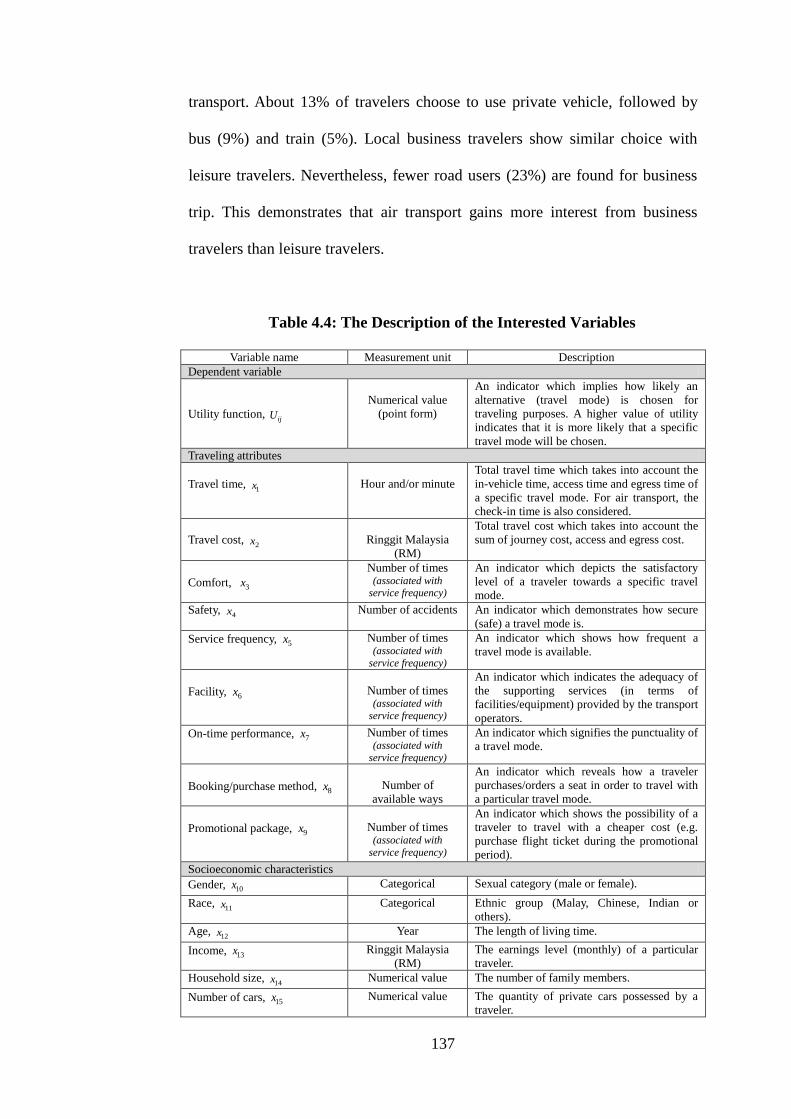
137

transport. About 13% of travelers choose to use private vehicle, followed by

bus (9%) and train (5%). Local business travelers show similar choice with

leisure travelers. Nevertheless, fewer road users (23%) are found for business

trip. This demonstrates that air transport gains more interest from business

travelers than leisure travelers.

Table 4.4: The Description of the Interested Variables

Variable name Measurement unit Description

Dependent variable

Utility function, ijU

Numerical value

(point form)

An indicator which implies how likely an

alternative (travel mode) is chosen for

traveling purposes. A higher value of utility

indicates that it is more likely that a specific

travel mode will be chosen.

Traveling attributes

Travel time, 1x

Hour and/or minute

Total travel time which takes into account the

in-vehicle time, access time and egress time of

a specific travel mode. For air transport, the

check-in time is also considered.

Travel cost, 2x

Ringgit Malaysia

(RM)

Total travel cost which takes into account the

sum of journey cost, access and egress cost.

Comfort, 3x

Number of times (associated with

service frequency)

An indicator which depicts the satisfactory

level of a traveler towards a specific travel

mode.

Safety, 4x Number of accidents An indicator which demonstrates how secure

(safe) a travel mode is.

Service frequency, 5x Number of times (associated with

service frequency)

An indicator which shows how frequent a

travel mode is available.

Facility, 6x


service frequency)

An indicator which indicates the adequacy of

the supporting services (in terms of

facilities/equipment) provided by the transport

operators.

On-time performance, 7x Number of times (associated with

service frequency)

An indicator which signifies the punctuality of

a travel mode.

Booking/purchase method, 8x

Number of

available ways

An indicator which reveals how a traveler

purchases/orders a seat in order to travel with

a particular travel mode.

Promotional package, 9x


service frequency)

An indicator which shows the possibility of a

traveler to travel with a cheaper cost (e.g.

purchase flight ticket during the promotional

period).

Socioeconomic characteristics

Gender, 10x Categorical Sexual category (male or female).

Race, 11x Categorical Ethnic group (Malay, Chinese, Indian or

others).

Age, 12x Year The length of living time.

Income, 13x Ringgit Malaysia

(RM)

The earnings level (monthly) of a particular

traveler.

Household size, 14x Numerical value The number of family members.

Number of cars, 15x Numerical value The quantity of private cars possessed by a

traveler.

138

Trans-border leisure travelers are found to have the highest tendency

(36%) in using air transport for which LCC (20%) is preferred than FSC

(16%). Among the ground transport, private vehicle is the most likely option

with the choice probability of 32%, followed by single-decker bus (20%),

double-decker bus (5%) and train (4%). Besides, air transport dominates the

market of trans-border business trip for which FSC (53%) is favored compared

to LCC (15%). The private vehicle again dominates the ground transport with

its choice probability of 15%. Bus and train are not preferred by business

travelers.

Table 4.5: The Choice Probability of Local and Trans-border Trips (%)

Local trip (KL-Penang) Trans-border trip (KL-Singapore)

Travel mode Leisure trip Business trip Leisure trip Business trip

FSC (MAS) 49.06 59.57 16.52 53.15

LCC (AirAsia) 24.05 17.06 20.34 15.02

Bus (single-decker) 9.04 8.08 20.66 8.09

Bus (double-decker) - - 5.81 5.04

Private car 13.30 10.70 32.31 15.11

Train 5.02 4.60 4.37 3.60

4.2.6 Analysis of LCC's Impacts on Mode Choice Decision

Tables 4.6 and 4.7 present multinomial logit models developed from the

stated preference survey of local and trans-border trips, respectively. The

models are statistically significant at 95% confidence level from the

perspectives of socioeconomic factors as well as the traveling attributes of

transport operators. All models are examined with the same socioeconomic

backgrounds of travelers and also on nine traveling attributes as described

139

earlier. The results show that the models are statistically significant towards

different traveling factors. Based on these models, the impacts of LCC on

mode choice decision is investigated and presented in the following sub-

sections.

4.2.6.1 Impact of LCC on FSC

The results show that the major factor that encourages trans-border

leisure trip makers to choose LCC over FSC is low travel cost. This is similar

to the findings of O‟Connell and William (2006) and Mohd Suki (2014).

However, for local leisure trip, travelers prefer FSC more than LCC (as the

utility constant of FSC is higher than LCC). This is because FSC could offer a

better comfort level compared to LCC. For trans-border business trip, the travel

cost remains as the major factor that encourages travelers to choose LCC.

However, most of the trans-border business travelers opt for FSC than LCC

most probably owing to the company‟s policies (normally larger firms) in

taking FSC due to the frequent flyer initiatives. This fact could be supported by

the occupation of respondents for which more than 50% of the respondents (as

shown in Table 4.3) are holding the position as government servant, executive

and professional, which are most likely working in large-scaled companies

which prefer FSC than LCC. This finding is in accordance with the results of

Evangelho et al. (2005) and O'Connell and Williams (2005, 2006). Besides, it

was found that comfort is the major factor for local business trip. The estimated

140

parameter shows that LCC is able to increase their mode share if the comfort

level could be improved (more significant than FSC since the value is higher).

For trans-border leisure trip, a sensitivity analysis is performed to

investigate the impact of the changes of travel cost on the mode share. The

results are displayed in Table 4.8. The results show that if the travel cost of

LCC decreases by 10% to 50%, the choice probability of LCC is estimated to

increase 2.71%-18.39%, with an average of 10.12%. In addition, this would

attract an additional of 2.22% of FSC travelers to LCC. For local business trip,

the results of sensitivity analysis as illustrated in Table 4.9 signify that if the

comfort level of LCC improves gradually (from 10% to 50%), the market share

of LCC could increase at an average of 4.24%. Specifically, the improvement

in comfort means that transport operators aim to ensure that their travelers

would use and enjoy more facilities/services. In such a case, transport operators

may provide some on-board facilities so that travelers could feel more relax

and comfortable during their travel. For instance, electric train services (ETS)

train is equipped with LCD TV particularly for the informative and relaxation

purposes. Accordingly, the higher level of improvement of comfort level refers

to more facilities/services that can be enjoyed by travelers during their travel.

Similarly, the reduction of travel cost, the adjustment (i.e. improvement) of the

comfort level at a higher level (i.e. from 10% to 50%) would increase the

market share of the LCC at a greater extent (i.e. from 1.26% to 7.45%).

Besides, it could be seen that the improvement of LCC's comfort level attracts

an average of 3% of FSC travelers.

141

Table 4.6: The Modeling Results of KL-Penang Trip (Local Trip)

Leisure trip Business trip

Parameter Coefficient t-statistic Coefficient t-statistic

ConstantMAS 2.6159 3.613 2.9045 3.961

ConstantAirAsia 1.3013 44.657 1.0904 28.490

ConstantBus -0.0645 -9.533 -0.4927 -16.918

GenderMAS -0.0725 -7.690 -0.0943 -15.773

GenderAirAsia -0.0679 -38.375 - -

GenderBus -0.2689 -119.756 -0.2171 -11.056

GenderCar 0.1007 383.864 0.0946 10.733

GenderTrain 0.3085 21.484 0.2809 136.089

RaceMAS - - -0.1190 -548.728

RaceCar - - -0.0371 -36.963

TimeCar -0.0091 -18.411 -0.0103 -1.640

ComfortMAS 0.1317 5.941 0.1918 12.643

ComfortAirAsia - - 0.2570 13.140

ComfortBus 0.0823 55.978 - -

SafetyBus 0.0292 17.039 - -

Log-likelihood function -2611.500 -2606.650

p-value 0.0319 0.0161

Number of observations 2,216 2,216

Table 4.7: The Modeling Results of KL-Singapore Trip

(Trans-border Trip)

Leisure trip Business trip

Parameter Coefficient t-statistic Coefficient t-statistic

ConstantMAS 2.0219 2.281 3.9085 4.387

- ker ConstantSingle dec bus 2.5810 378.929 3.0808 448.562

IncomeMAS 0.1469 17.355 0.2057 18.668

IncomeAirAsia 0.0343 37.583 - -

- ker IncomeSingle dec bus -0.1480 -157.429 -0.0084 -15.949

- ker IncomeDouble dec bus -0.1969 0.0379 -0.4571 -18.218

IncomeCar 0.0785 118.149 0.1157 172.681

IncomeTrain 0.0852 1.956 0.1442 4.602

CostAirAsia -0.0046 -3.229 -0.0073 -7.190

- ker CostDouble dec bus - - -0.0181 -4.025

CostTrain -0.0206 -16.327 -0.0402 -83.191

SafetyAirAsia - - 0.0124 2.309

- ker SafetySingle dec bus 0.0117 5.078 - -

Log-likelihood function -3380.697 -2944.421

p-value 0.0000 0.0000

Number of observations 2,222 2,224

142

Table 4.8: The Sensitivity Analysis of KL-Singapore Trip

(Trans-border Leisure Trip)

Travel cost of AirAsia -10% -20% -30% -40% -50% Average

Choice probability

(%)

MAS -0.61 -1.32 -2.13 -3.04 -4.01 -2.22

AirAsia +2.71 +5.95 +9.69 +13.88 +18.39 +10.12

Single-decker bus -0.41 -0.87 -1.40 -1.98 -2.61 -1.45

Double-decker bus -0.20 -0.43 -0.71 -1.02 -1.36 -0.74

Car -1.37 -3.02 -4.96 -7.13 -9.47 -5.19

Train -0.14 -0.30 -0.49 -0.70 -0.94 -0.51

Table 4.9: The Sensitivity Analysis of KL-Penang Trip

(Local Business Trip)

Comfort level of AirAsia +10% +20% +30% +40% +50% Average

Choice

probability

(%)

MAS -0.92 -1.92 -3.00 -4.17 -5.42 -3.09

AirAsia +1.26 +2.64 +4.13 +5.73 +7.45 +4.24

Bus -0.12 -0.26 -0.40 -0.56 -0.73 -0.41

Car -0.15 -0.31 -0.48 -0.67 -0.87 -0.50

Train -0.07 -0.15 -0.24 -0.33 -0.43 -0.24

4.2.6.2 Impact of LCC on Ground Transport

For local business trip, the comfort of LCC is found to be significant.

This reveals that local business travelers tend to fly with LCC, which is

anticipated to have a better comfort level (probably due to shorter travel time)

compared to the ground transport (i.e. private car, bus, train). For local trip

(both leisure and business purposes), the fact that LCC is preferred is also

supported by the constant of LCC which has a higher value compared to the

constant of bus. For trans-border trip (both leisure and business purposes),

travel cost emerges as the major cause that encourages travelers to travel with

LCC. In addition to travel cost, safety appears as the significant determinant for

143

trans-border business travelers in choosing LCC. LCC is preferred most

possibly owing to the least accident occurrence compared to ground transport

(as shown in Table 4.2). Furthermore, there might be a negative perception of

travelers towards the safety of group transport, especially car and bus due to

increasingly road accidents from year to year (MIROS, 2012). This supports

the decision-making of business travelers who have a concern for safety.

The findings of sensitivity analysis for trans-border leisure trip and

local business trip (as displayed in Tables 4.8 and 4.9), respectively show that

the adjustment of travel cost and comfort level could increase the mode share

of LCC. If the travel cost of LCC decreases (10%-50%), the choice probability

of LCC is estimated to increase gradually with an average of 10.12%, by

shifting about 8% of the users of ground transport (i.e. 5% of car users, 2% of

bus users and about 1% of train users). Besides, the findings show that if the

comfort level of LCC improves gradually (10%-50%), the market share of

LCC could increase at an average of 4.24% for which the improvement of the

comfort level at a higher level would increase the market share of the LCC

with a greater proportion. However, the impact of the improvement of comfort

level in mode shifting is lesser compared to the reduction of travel cost, i.e. this

strategy (improvement of comfort level) would only attract about 1.15% of the

users of ground transport.

144

4.2.6.3 Effect of Socioeconomic Background

From the mode choice analysis, it was found that one of the significant

factors that could influence travelers‟ mode choice is their socioeconomic

background. Table 4.6 shows that gender is a significant factor that affect

leisure and business travelers of local trips. The results show that male travelers

prefer to travel with air transport and bus while car and train are the likely

options among female travelers. Besides, mode choice decision is also affected

by the race factor. Malay and Chinese travelers show a high tendency in

traveling with FSC and car. From Table 4.6, it could be seen that respondents‟

income level is another significant factor for leisure and business trips. It

shows that those with higher income tend to travel with air transport or private

vehicles. On the other hand, those with lower income show a tendency to travel

with bus, most probably due to cheaper travel cost.

4.2.7 Implications for Managerial Practices

For airlines, mode choice analysis is particularly crucial from three

major managerial perspectives, i.e. demand, supply and sustainability as listed

as follows:

145

From the aspect of demand:

to manage travel demand properly

to predict future travel trend precisely

to develop and implement appropriate marketing strategy considerably

to attract new travelers (to increase mode share) effectively

From the aspect of supply:

for operations and performance enhancement (to improve existing

services and systems)

for services planning (to meet travelers' demand and expectations)

for fleet planning decision-making (to support operating networks)

From the aspect of sustainability:

to retain the loyalty of travelers

to outperform competitors (under multimode transportation system)

to assure profitable operations and market shares

4.2.8 Summary

A proper understanding of travelers‟ mode choice decision in

multimode transport network is important for an efficient planning. It is a

crucial step to predict the usage of transport facilities and to manage travel

demand effectively. While most of the studies focus on the analysis for the

146

developed countries, this research investigates travelers‟ mode choice decision

in the developing countries. Besides studying the choices between LCC and

FSC, this research also aims to deliberate the competition between LCC and

ground transport. A stated preference survey is carried out to investigate

travelers‟ choice for local and trans-border trips. Multinomial logit models are

developed to identify the underlying factors that contribute to mode choice. It

was found that a few influential factors that could affect mode choice decision

are trip purpose, traveling destination, travel cost, comfort, safety, and

travelers‟ background. It was also found that LCC is only preferred by those on

trans-border leisure trip. For those who choose LCC, low travel cost is their

main concern. Other travelers choose FSC due to its excellent comfort level.

Most of the travelers who choose to use ground transport prefer to travel with

their own private vehicles for more flexibility and comfort. However, for those

who choose to use buses, travel safety has become their main concern. A

sensitivity analysis is carried out to study the impact of changes of travel cost

and comfort level on LCC. The results show that the LCC is able to attract a

substantial amount of travelers from FSC and ground transport if the ticket

price is reduced while the comfort level is increased. As such, it could be seen

that mode choice analysis could provide informative highlights to airlines for

services enhancement (including how to provide a strategic fleet planning as

discussed in the following section). Therefore, in order to capture the mode

choice of travelers properly, those aspects as discussed earlier should be

handled wisely.

147

4.3 Analytic Hierarchy Process (AHP) Modeling Framework

4.3.1 The Role of Analytic Hierarchy Process (AHP) In Fleet Planning

Decision-Making

While providing an adequate fleet supply, it is important to capture

mode choice analysis (traveler‟s response) in view of the fact that air

travelers (passengers) are the main users of airline's services which constitutes

the market share and main income to airlines. Furthermore, traveler‟s behavior

was changing with extensive growth of multimode transportation networks. As

such, how airlines make an optimal fleet planning decision, i.e. a multiple

criteria decision-making, throughout the planning horizon is important to meet

travel demand profitably at a desired service level. Therefore, the fleet planning

decision-making of airlines which is, in fact, uncertain (primarily due to

stochastic demand) and greatly governed by various key aspects (multi-criteria)

could be solved strategically with the aid of the AHP.

By allowing the respective judgments to vary over the values of a

fundamental scale of 1-9, AHP possess the capability to capture the fuzziness

(uncertainty) in making a multi-criteria decision (Saaty and Tran, 2007).

Specifically, the judgments made with AHP, in the form of pair-wise

comparison, by using judgment scale 1-9 are fuzzy (uncertain). As such, the

148

fleet planning decision-making of airlines which is, in fact, uncertain could be

solved by making use AHP suitably. Comparatively, AHP is widely used due to

its ease of use as well as its straightforward scalable and understandable

manner than any other multi-criteria decision making methods (Velasquez and

Hester, 2013). More importantly, AHP which is able to capture the fuzziness

and vagueness (uncertainty) explicitly could reflect realistically the fleet

planning problem of airlines in a better manner. To the best of the authors'

knowledge, this research is the first that integrates AHP and mode choice

modeling in solving the fleet planning problem explicitly. The developed

methodology is capable to show how various key aspects affect fleet planning

decision-making, i.e. how fleet planning (a multi-criteria decision) is made to

meet stochastic demand.

4.3.2 Modeling Framework

The proposed modeling framework of AHP basically involves three

major stages as displayed in Figure 4.2. Stage 1 involves the judgment and

comparison among decisional criteria while Stage 2 focuses on the judgment

and comparison among the key aspects for each decisional criteria. Finally,

Stage 3 computes the end result which is the probability of the key aspect that

influence the fleet planning decision-making. For Stage 1, the modeling

framework commences by evaluating the relative comparison of n decisional

criteria with a comparison scale of 1-9 (Saaty, 1980, 1994). Typically, the

149

relative comparison is presented in the form of a matrix, i.e. a square matrix

with a size of x n n . In other words, the matrix is playing the role to reflect the

subjective judgment of decision makers towards the relative comparison of n

decisional criteria. For x n n matrix, the diagonal element which is the

comparison of n decisional criteria against itself is always equal to 1 while

other elements in the matrix signify the relative comparison of n decisional

criteria. For x n n matrix, it is observable that 1

ij

ji

aa

for which ija defines

the element at row i and column j of the matrix. This shows that the element

ija and

jia are the reciprocal of each other. As such, the x n n matrix is also

known as reciprocal matrix.

It is important to note that some degree of inconsistency is expected due

to the fact that the decision-making is made based on the subjective judgment

of decision makers. Therefore, the consistency of the matrix needs to be

examined accordingly. This can be done by conducting a consistency test.

Mathematically, the matrix is said to be consistent if x , , ij jk ika a a i j k .

Generally, there are three components, namely consistency ratio (CR),

consistency index (CI) and random consistency index (RI) that are required to

carry out the consistency test. Basically, CR evaluates the ratio of CI and RI of

the matrix in such a way that CI measures the consistency of the matrix by

making use of the deviation of the eigenvalue and matrix size while RI is the

average CI of a large sample of randomly generated matrices. The matrix is

said to be consistent if CR < 0.1. To examine the consistency, the largest

150

eigenvalue of the matrix, max also acts as a consistency indicator for which the

matrix is said to be more consistent if the value of max

is getting closer to

matrix size (Saaty, 1990).

Figure 4.2: The Modeling Framework to Quantify the Probability of Key

Aspect

At stage 2, a similar procedure (as in stage 1) is carried out to form the

judgment matrix that reflects the relative comparison among the key aspect for

each decisional criteria. As addressed earlier, the key aspect refers to a

particular perspective (concern) that could affect the fleet planning decision-

making. By validating the consistency of matrix, subsequently the output of

AHP approach is computed (at stage 3) to quantify the probability of the

respective key aspect. The aspect with a higher probability is interpreted to be

more essential than other aspect with a lower value. Note that the total of

probability is one, i.e. 100% as the full decision of airlines. The decision-

making in fleet planning shall then be driven by the resultant probability of key

151

aspects.

The modeling framework of AHP (embedded with mode choice

modeling) as outlined in Figure 4.2 can be carried out as follows:

For stage 1:

I. Determine decisional criteria, i

C

To make fleet planning decision, decisional criteria, , 1,...,i

C i n can

be identified appropriately by identifying the relevant element that could affect

the decision-making of airlines. Generally, the elements that are found to affect

airlines are decision policy of airlines, consultancy of experts/consultants, past

performance of airlines and travelers‟ response in view of their influential

impacts in fleet planning (AirAsia Berhad, 2004; KPMG, 2007; Lessard, 2012;

Malaysia Airlines, 2010a; Ryanair, 2012).

II. Establish judgment matrix (for n decisional criteria)

A pair-wise comparison matrix, A involving n decisional criteria (as

determined from step I) can be expressed as follows (Saaty, 1980):

12 1

212

1 2 x

1

1 1

1 1 1

n

n

n n n n

a a

aa

A

a a

(4.10)

Generally, matrix A is governed by 1

>0, 1, ij ii ij

ji

a a aa

for ,i j . To assure

152

consistency, note that x , , ij jk ik

a a a i j k . Specifically, ija implies the

relative comparison of criteria i over j based on judgment scale 1-9 (for which

1:equal importance, 3:weak importance of one over the other; 5:strong

importance; 7:demonstrated importance; 9:absolute importance while 2, 4, 6

and 8 signify the corresponding intermediate values between two adjacent

judgment (Saaty, 1977, 1980, 1990)).

In real practice, decision makers are likely to make an inconsistent

comparison (judgment). To handle this issue, the following actions could be

done (Saaty and Tran, 2007):

(1) Identify the most inconsistent judgment in the matrix and determine the

range of values for which the inconsistency could be improved.

(2) Request the decision maker to consider if he/she can alter his/her judgment

to a possible value in that range. Otherwise, the decision is postponed until

a better understanding is obtained.

(3) Same procedure could be repeated by examining the second most

inconsistent judgment and so on.

III. Calculate the largest eigenvalue

As an indicator for consistency, the largest eigenvalue, max of matrix A

can be determined as follows (Saaty, 1990):

max

1

nj

ij

j i

wa

w

(4.11)

153

for which ij

a is the element of matrix A while i

w and j

w respectively

represent the average of row i and j of matrix A. Note that a matrix is said to be

more consistent if the value of the largest eigenvalue is getting closer to matrix

size.

IV. Perform consistency test (for matrix A)

Consistency test is needed to assure the consistency of matrix A (with

size n). This test can be conducted based on the consistency index, CI and

random consistency index, RI which are outlined as follows (Saaty, 1977):

max

1.98 2,

1

nnCI RI

n n

(4.12)

Saaty (1977) showed that max

n if the matrix does not include any

inconsistency. This implies that the closer the value of max to n, the matrix is

more consistent.

By using the measurement of CI and RI, the consistency ratio, CR can

be evaluated as follows:

CI

CRRI

(4.13)

As shown in Equation (4.13), CR compares the consistency index, CI of the

matrix and a purely random matrix, RI. The judgment matrix is said to be

consistent if CR < 0.1.

154

For stage 2:

V. Establish judgment matrix of key aspect (for each decisional criteria)

For airlines, key aspect k

s signifies the relevant aspect (concern) that

could affect fleet planning decision-making. Specifically, the probability of key

aspect reflects the likelihood or degree of each perspective in making an

optimal fleet planning decision. As such, how to capture these key aspects for

decision-making is vital. It is important to note that the number of key aspect to

be captured may vary among airlines. For instance, some airlines claim that the

aspects of operational and economy are two major determinants in fleet

planning (AirAsia Berhad, 2010a; Malaysia Airlines, 2010a). In addition, the

environmental aspect should be taken inconsideration due to its increasing

concern and impacts on airline‟s operations. In such a case, three key aspects

namely 1 2, s s and 3

s could be defined accordingly to capture the aspect of

operational, economy and environmental, respectively. For airlines, operational

aspect ( 1s ) particularly refers to relevant perspectives such as the ability to

secure traffic rights and operating difficulties of aircraft type while the

economy aspect ( 2s ) covers the financial benefits of shareholders, economic

benefits of new aircraft and so on. For the environmental aspect ( 3s ), the fuel

efficiency of airlines is included in view of the fact that lesser fuel consumption

produces fewer emission (Williams et al., 2002). In fact, these aspects

(operational, economy and environmental) are closely related to one another

owing to the fact that aircraft operations of airlines in supporting the operating

networks would greatly affect not only the financial gains of airlines but also

their green (environmental) performance in terms of fuel efficiency, aircraft

155

emission and noise.

By considering k key aspects, i.e. 1,...,

ks s and decisional criteria

iC ,

the pair-wise comparison matrix of the key aspect (for each decisional

criteria), iC

B can be formed as follows:

12 1

212

1 2

1

1 1

1 1 1

n

n

Ci

n n kxk

s s

ss

B

s s

(4.14)

for which matrix iC

B is a square matrix with size k x k while ij

s reflects the

relative comparison of key aspect i

s over js .

In order to obtain the pair-wise comparison matrix of the key aspect

1,...,

ks s for the decisional criteria of travelers‟ response, travel survey and

mode choice analysis can be done as follows:

Step 1: Conduct travel survey

Travel survey can be undertaken necessarily by airlines to examine the

preference of travelers as well as its impacts in fleet planning. Specifically,

travel survey for different trip purpose (e.g. leisure or business) can be carried

out for different destination (e.g. local or trans-border). Traveler‟s response via

survey could reveal their preferences and travel behavior in a better manner.

156

Step 2: Conduct mode choice analysis

The response of travelers via travel surveys (input) could be utilized to

generate the mode choice modeling models (output). The estimated parameters

of respective trip (e.g. local leisure trip, local business trip, trans-border leisure

trip and trans-border business trip) which constitute the mode share of

respective operating network can be obtained accordingly from the mode

choice modeling analysis.

Step 3: Evaluate the ratio of key aspect to form judgment matrix, iC

B

For the decisional criteria of travelers' response, the pair-wise comparison

matrix of key aspect 1,...,

ks s can be evaluated by taking into account the mode

share analysis (from step 2). Subsequently, the mode share of operating

network which corresponds to the respective key aspect can be evaluated

accordingly to obtain the relative comparison of key aspect. To do this, the

relevant components of each key aspect, w

SkF are taken into account to assess

the relationship of the operating network, d

Net and corresponding key aspect,

ks . This is necessary to examine the impacts between operating network and

key aspect (to work out the ratio of key aspect). The detail framework to

evaluate the ratio of key aspect is shown in Figure 4.3.

By considering W relevant components of key aspect and also P

operating networks, the respective ratio of key aspect (to form judgment matrix

157

CiB ) can be computed as follows:

: , , 1,..., ; 1,..., ; 1,...,

w

d Si

i j w

d S j

Net Fs s i j k w W d P

Net F

(4.15)

where d

Net refers to operating network and w

SkF denotes the relevant

component of key aspect, k

s .

Figure 4.3: The Evaluation of the Ratio of Key Aspect

VI. Perform consistency test (for matrix iC

B )

The consistency of matrix, Ci

B can be confirmed by adopting a similar

procedure as described in stage 1, i.e. the matrix is said to be consistent if

0.1CR .

158

For stage 3:

VII. Compute the probability of key aspect

The probability of key aspect can be evaluated as follows (Saaty, 1980):

* *Probabilityi r

A B (4.16)

where *

iA represents the average of row 1, 2,...,i n (i.e. decisional criteria) of

normalized matrix A while *

rB denotes the average of row 1, 2,...,r k (i.e.

key aspect with regard to each decisional criteria) of normalized matrix iC

B .

4.3.3 Numerical Example

This section illustrates the applicability of the developed framework

(with mode choice modeling) to quantify the probability of the respective key

aspect in making an optimal fleet planning decision.

I. Determine decisional criteria, i

C

Based on publicly accessible published reports (AirAsia Berhad, 2004;

KPMG, 2007; Lessard, 2012; Malaysia Airlines, 2010a; Ryanair 2012), four

decisional criteria, namely the decision policy of airline (DP), consultancy of

experts (CE), past performance of airline (PP) and travelers‟ response (TR) are

identified as the major key aspect that could affect the fleet planning decision

of airlines. The elements of DP, CE, PP and TR are denoted as criteria

159

1 2 3, , C C C and

4C respectively. Specifically, the decision policy of airlines

(DP), 1

C refers to a particular course of action for airlines to make operational

and managerial decision (including fleet planning decision). For instance,

airlines may standardize their fleet choice in terms of aircraft type primarily

due to financial and operational concerns. For airlines, the consultancy of

experts (CE), 2

C refers to advices or judgments of consultants/panels towards

airline's operating performance, financial management as well as decision-

making. In supporting the servicing networks, the past performance of airline

(PP), 3

C includes the perspectives of demand and supply for which demand

perspective takes into account the travel trend while the perspective of supply

considers the fleet performance in servicing available operating networks.

From the perspective of the users of air transport system, the travelers‟

response (TR), 4C focuses on the mode choice modeling of travelers which

reveals the behavior and perception of travelers towards the services of airlines.

II. Establish judgment matrix (for n decisional criteria)

Based on the decisional criteria of 1 2 3, , C C C and 4

C as identified in

Step I, judgment matrix A can be formed as follows:

4 4

1 0.75 0.57 1.00

1.33 1 0.77 1.32

1.74 1.29 1 1.68

1.00 0.76 0.60 1x

A

To obtain matrix A, accessible published information is compiled with the aid

of a simulation approach for which the simulated data (in Table 4.10)

160

represents the relative comparison of 10 managerial experts towards the

decisional criteria i

C over j

C . As shown in Table 4.10, the judgments of

experts are compiled suitably as geometric mean (Aczel and Saaty, 1983).

III. Calculate the largest eigenvalue

The largest eigenvalue, max of matrix A can be determined as follows:

max

1

4.0001n

j

ij

j i

wa

w

The value of the largest eigenvalue is coherent with the fact of Saaty (1977) for

which max

n .

IV. Perform consistency test (for matrix A)

Since 4n (i.e. size of matrix A), the element of CR is computed as

follows:

5

54.1 x 104.2 x 10

0.99

CICR

RI

Thus, the consistency is acceptable because 0.1CR . This signifies that the

matrix A is consistent (reliable) in terms of the judgment (evaluation) of

decision makers.

161

Table 4.10: The Evaluation of Relative Comparison

Expert, k 1 2 3 4 5 6 7 8 9 10 Geometric

mean

12a 0.71 0.6 0.76 0.75 1.02 0.69 0.79 0.81 0.93 0.57 0.75

13a 0.63 0.67 0.56 0.51 0.44 0.62 0.63 0.8 0.51 0.47 0.57

14a 1.03 0.94 0.96 0.92 1.01 0.96 1.07 0.97 1.01 1.15 1.00

23a 0.81 0.86 1.01 0.75 0.69 0.76 0.83 0.54 0.9 0.69 0.77

24a 1.26 1.33 1.23 1.27 1.46 1.25 1.36 1.36 1.37 1.35 1.32

34a 1.7 1.51 1.61 1.63 1.86 1.72 1.81 1.77 1.46 1.75 1.68

V. Establish judgment matrix of key aspect (for each decisional criteria)

To form the matrix of traveler‟s response (TR), the following procedure

can be conducted:

Step 1: Conduct travel survey

Four stated preference travel surveys had been undertaken in 2011 (as

discussed earlier) in order to model the mode choice decision of travelers.

These surveys aim to identify and analyze the preference of travelers towards

the ground transport (bus, car and train) and air transport (FSC and LCC).

These surveys are denoted as 1 2 3, , y y y and 4y for local leisure trip, local

business trip, trans-border leisure trip and trans-border business trip,

respectively. Generally, the operating networks of airlines can be categorized as

short-haul and medium/long-haul networks. In such a case, local leisure trip

( 1y ) and local business trip ( 2y ) as domestic flights are classified as short-haul

network (1

Net ) while trans-border leisure trip ( 3y ) and trans-border business

trip ( 4y ) are included for medium/long-haul network (2

Net ). These networks

are then utilized to evaluate the ratio of key aspect, ks (as described further in

162

Step 3).

Step 2: Conduct mode choice modeling

The response of travelers via travel surveys (input) are then adopted to generate

the mode choice modeling models (output). The results of mode choice

analysis are summarized in Table 4.11.

Table 4.11: The Modeling Results of Travel Survey

Network Short-haul network,

1Net Medium/long-haul network, 2Net

Attribute

Local leisure

trip, 1y

Local business

trip, 2y

Trans-border

leisure trip, 3y

Trans-border

business trip, 4y

Mode choice of trip

36.5550 38.3150 18.4300 34.0850

Average mode choice 37.4350 26.2575

Step 3: Evaluate the ratio of key aspect to form judgment matrix, TR

B

As shown in Table 4.12, the mode share of respective network which

correspond to the aspect of operational ( 1s ), economy ( 2

s ) and environmental

( 3s ) of airlines are evaluated accordingly to compare with the respective key

aspect. To do this, the relevant components of each key aspect, k

w

SF are taken

into account to assess the relationship of the operating networks, d

Net and

corresponding aspect, ks . As mentioned earlier, the relevant components of

operational aspect ( 1s ) of airlines may refer to several perspectives, including

the number of passengers carried and the load factor in servicing operating

networks. On the other hand, the economy aspect of airlines ( 2s ) may cover

163

numerous components, including the operating revenue and available capacity

(seats) while the environmental aspect (3

s ) captures the fuel consumption of

airline in response to fuel efficiency of the operating networks. The data of

these aspects are compiled based on the operating performance of Malaysia

Airlines (Malaysia Airlines, 2010a). The evaluation of the ratio of respective

key aspect is shown in Table 4.12.

Table 4.12: The Evaluation of the Ratio of Key Aspect

(For Traveler's Response)

Key aspect

1s

(operational)

Key aspect 2s

(economy)

Key aspect 3s

(environmental)

Operating

network

Average

mode

choice

Load

factor,

1

1

SF

Passengers

carried,

1

2

SF

Revenue

passenger

kilometers

(RPK), 2

1

SF

Available

seats

kilometers

(ASK), 2

2

SF

Fuel

efficiency,

3

1

SF

Short-haul, 1Net 37.4350 50% 45% 10% 10% 68%

Medium/long-

haul, 2Net

26.2575 50% 55% 90% 90% 32%

k

w

d SNet F 63.1336 54.7505 33.8582

Ratio of key aspect 1 2 1 3 2 3: 1.15, : 1.86, : 1.62s s s s s s

By having the ratio of key aspect, the judgment matrix of travelers‟

response, TRB could be formed as follows:

3x3

1 1.15 1.86

0.87 1 1.62

0.54 0.62 1

TRB

As mentioned earlier, there are three more decisional criteria, i.e. decision

policy of airline (DP), consultancy of experts (CE) and past performance of

airline (PP). The judgment matrices of these decisional criteria are assumed to

be as follows (due to the lack of accessible data):

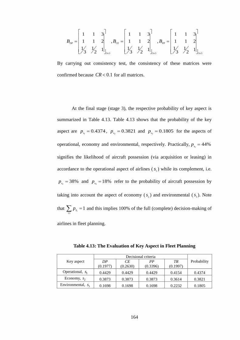
164

3x3 3x3 3x3

1 1 3 1 1 3 1 1 3

1 1 2 , 1 1 2 , 1 1 2

1 1 1 1 1 11 1 13 2 3 2 3 2

DP CE PPB B B

By carrying out consistency test, the consistency of these matrices were

confirmed because 0.1CR for all matrices.

At the final stage (stage 3), the respective probability of key aspect is

summarized in Table 4.13. Table 4.13 shows that the probability of the key

aspect are 1

0 4374s

p . , 2

0.3821s

p and 3

0.1805s

p for the aspects of

operational, economy and environmental, respectively. Practically,1

44%s

p

signifies the likelihood of aircraft possession (via acquisition or leasing) in

accordance to the operational aspect of airlines (1

s ) while its complement, i.e.

238%

sp and

318%

sp refer to the probability of aircraft possession by

taking into account the aspect of economy (2

s ) and environmental ( 3s ). Note

that 1iS

i

p

and this implies 100% of the full (complete) decision-making of

airlines in fleet planning.

Table 4.13: The Evaluation of Key Aspect in Fleet Planning

Key aspect

Decisional criteria

Probability DP

(0.1977)

CE

(0.2630)

PP

(0.3396)

TR

(0.1997)

Operational, 1s 0.4429 0.4429 0.4429 0.4154 0.4374

Economy, 2s 0.3873 0.3873 0.3873 0.3614 0.3821

Environmental, 3s 0.1698 0.1698 0.1698 0.2232 0.1805

165

4.3.4 An Application in Solving Fleet Planning Problem

In such a complicated air transportation system, airlines encounter

many challenging unexpected events which are unpredictable in nature. In

accordance to the occurrence of unexpected events (risks), an efficient fleet

planning is necessary. As such, the probable phenomena, 1,...,

ks s for a total of

k phenomena are defined to describe the possible key aspect of aircraft

possession in meeting stochastic demand under uncertainty. The probability of

probable phenomena, 1,...,

ks sp p quantifies the likelihood (probability) of

respective key aspect (determinant) in making fleet planning decision via

aircraft acquisition/leasing. In other words, they define how the fleet supply

(aircraft composition) is made to meet travel demand. Preferably, the quantity

of aircraft should be available adequately (at a right time) for a strategic fleet

planning decision. If probable phenomena and its probability are not defined, it

means that airlines only deals with one possible aspect to meet stochastic

demand, i.e. they have perfect confidence that a certain level of stochastic

demand will be met by considering a single aspect only. However, this should

not be the case because the actual decision-making process is subject to

multiple criteria (aspects). Furthermore, the decision-making may vary from

time to time under uncertainty. As such, this indicator is necessary in fleet

planning. The number of probable phenomenon varies depending on the

perception and consideration of airlines. In this research, three key aspects

(probable phenomena), namely operational, economy and environmental are

considered.

166

4.3.5 Fleet Planning Decision Model

In general, the airline's profit is contributed by the total revenue and the

total operating cost. For operating period t, the total revenue, ( )P L

t tTR I I can

be expressed as follows:

1

1 1

for 1,..., ; ,...,n m

P L S S

t t t t tiy tiy k

i y

TR I I E fare D sold resale t T S s s

(4.17)

For Equation (4.17), the first term on the right-hand side indicates the expected

income from the sales of flight tickets while the second term denotes the

revenue from the sales of aging aircraft.

On the other hand, the total operating cost, ( )P L

t tTC I I of airlines can

be formed as follows:

1 1 1 1 1

1 1 1 1 1

cos ,

for 1,..., ;

n n n n mP L S S P L S i P P

t t t t ti ti ti ti ti t t tiy tiy

i i i i y

n m n n nL L P L

tiy tiy ti ti ti ti ti

i y i i i

TC I I E t D u purc x lease x hgf D A I dep

I dep dp x dl x C fuel t T S

1,...,

ks s

(4.18)

The terms on the right-hand side of Equation (4.18) signify the expected cost of

flight, aircraft purchase cost, lease cost, maintenance cost, depreciation

expenses, payable deposit of aircraft acquisition/leasing and fuel expenses,

respectively.

167

In summary, fleet planning model of airlines of operating period

1,..., t T can be presented as follows:

1

1

...1max

1t

k

P L P L

s t t t tP L

t t tX P L P L P L

t s t t t t t t t

p TR I I TC I IP I I

r p TR I I TC I I P I I

(4.19)

subject to:

Budget constraint: ( )

1 1

n nP L


i i

purc x lease x MAX

(4.20)

Demand constraint: 1

, 1n

t S i S

i t t t

i

SEAT f D A D

(4.21)

Sales of aircraft constraint: ( 1) ( 1)

P

tiy t i ysold I

(4.22)

Lead time constraint: 1 1 ti LT LT

DLT F (4.23)

Selling time constraint: 1 1ti ST ST

DST F (4.24)

where , , , , , , , 0S P L P L

t t t t t t t tD X X I I SOLD O R Z . For model (4.19), budget

constraint ascertains whether if the solution is financially feasible for airlines

while demand constraint ensures that travelers‟ demand could be met

satisfactorily. The constraint of sales of aircraft ensures that the quantity of

aircraft sold is not more than the aircraft owned by airlines. Lead time

constraint and selling time constraint respectively indicate when airlines are

supposed to order new aircraft and release aging aircraft for sales. The term

1t

tr

is used for discounted value across the planning horizon while ks

p

indicates the probability of k-th probable phenomenon for having P

tI and L

tI as

initial fleet supply (aircraft possession). Specifically, the element of 1 2,

s sp p

and 3s

p respectively signifies the probability of operational, economy and

environmental aspect of airlines in making strategic fleet planning decision.

168

Mathematically, the developed optimization model, in the form of probabilistic

dynamic programming model, can be solved by decomposing it into a series of

simpler sub-problems by using backward workings mechanism.

4.3.6 Data Description

A case study consisting of three types of aircraft, i.e. A320-200, A330-

300 and B737-800 are considered for a set of OD pairs for a planning horizon

of eight years. Most of the data are compiled based on the available reports

(AirAsia Berhad, 2010a; Malaysia Airlines, 2010a; Airbus, 2010a, 2010b,

2010c; Boeing, 2012). For each operating period, the level of stochastic

demand is obtained by applying the 5-step modeling framework of stochastic

demand. Based on the AHP modeling framework, the probability of key

aspects (for the benchmark scenario) are 1

0 4374s

p . , 2

0.3821s

p

and

30.1805

sp

for the aspect of operational, economy and environmental,

respectively. The data input of benchmark scenario are listed as follows:

Three probable phenomena are considered, i.e. 3k

At t = 1, quantity of aircraft is 11 12 13

35P P PI I I and 11 12 13

0L L LI I I

At t = 1, quantity of aircraft to be three years old is 113 123 133

3P P PI I I

Budget, ( )

$6,500 millionbudget t

MAX

Discount rate, 5%t

r

Significance level of demand constraint, 5%

169

Significance level of lead time constraint, 5%

Significance level of selling time constraint, 5%

Deposit of aircraft acquisition, 10%t tn

DP purc

Deposit of aircraft leasing, 10%t tn

DL lease

Setup cost, 0ti

u

11 , 1 , 2, 3,.., i is ss

t t t tD D D α D i k (4.25)


2

2 4 222.57 9.776x10 7.83x10 [R 0.97]n n

t tf A A (4.26)

The function of traveled mileage is

22,066 2,875,383 [R 0.83]g f (4.27)


3 3 25.177x10 7.97x10 [R 0.94]h g (4.28)


5 2 27.46 8.3x10 98,572 [R 0.88]tn

C fuel f f (4.29)

The quantity of aircraft is

5 210 73.6 [R 0.92]NA NP (4.30)


In addition to benchmark scenario, two more scenario (as shown in Table 4.14)

are examined for further analysis to inspect relevant influential input in

generating strategic fleet planning decision.

170

Table 4.14: Further Analysis in Solving Fleet Planning Problem

Scenario Decisional

criteria

Description Judgment

matrix

P

Decision

policy

(DP)

The adjustment on the relative comparison

of key aspect is done in the form as

follows:

environmental operational economy 3x3

1 2 1

1 112 3

1 3 1

DPB

Q

Travelers‟

response

(TR)

The change of travelers‟ response is

investigated towards travel cost reduction

strategy. According to mode choice

analysis, the mode share was found to

increase 18.39% in response to the

strategy of airline (AirAsia) in reducing

50% of travel cost (airfare).

3x3

1 1.02 1.98

0.98 1 1.94

0.51 0.52 1

TRB

Note: For the relative comparison of key aspect, the benchmark scenario is outlined in such a way as follows:

operational economy environmental

Specifically, scenario P focuses on the changes of decision policy (DP)

of airline, i.e. from the aspect of supply. By allocating different weight

(priority) on operational, economy and environmental aspect in such a way that

the environmental aspect gains the highest concern (priority) in terms of the

decision policy of airline, followed by operational and economy aspects,

scenario P inspects not only the possible variation on the probability of the

respective key aspect (operational, economy and environmental) but also the

possible changes of decision-making in fleet planning. It is anticipated that the

resultant outputs are driven by the weight allocation of airline based on the

relevant decision policy (i.e. an influential decisional criteria in fleet planning).

Scenario Q inspects the perspective of demand in terms of the changes of

travelers' response (TR). By capturing the possible changes of mode choice

decision of travelers towards the services of airlines (i.e. travel cost reduction),

scenario Q inspects the impacts of demand level (in terms of choice

probability) in fleet planning, i.e. by quantifying the possible probability of

operational, economy and environmental aspects that could affect fleet

171

planning decision greatly. Specifically, traveler's response could be compiled

by undertaking various travel survey on the respective operating networks

(short-haul and medium/long-haul). It is anticipated that scenarios P and Q

would capture the supply-demand interaction in a greater and better manner.

4.3.7 Results and Discussion

4.3.7.1 Benchmark Problem versus Scenario P

The results of the case study are shown in Table 4.15 and 4.16 (with the

graphical results as displayed in Figure 4.4). The results imply that the

decisional criteria could affect the probability of the key aspects (operational,

economy and environmental), optimal profit of airline as well as fleet planning

decision-making. From the results of the benchmark scenario, it could be seen

that the relative comparison of key aspect for decisional criteria tends to

produce the probability of key aspect in about the same way. This could be

seen in Tables 4.14 and 4.15 for which the judgment matrix of benchmark

scenario which has the relative comparison of the key aspect in the form of

operational economy environmental would produce the probability of key

aspect in similar way, i.e. probability of operational aspect probability of

economy aspect probability of environmental aspect. Some changes to the

probability of key aspect could be seen in scenario P for which the adjustment

172

of the relative comparison of key aspect has been done with regard to the

decision policy of airline (while other decisional criteria remain unchanged).

Scenario P was outlined by putting more weight (relative comparison) on

environmental aspect instead of operational and economy aspect. Subsequently,

the results in Table 4.15 show that the probability of environmental aspect

increases about 30% while the probability of operational and economy aspects

decreases (compared to benchmark scenario). However, the probabilities of

operational and economy aspects are still higher compared to environmental

aspect. This happens because the resultant probability of key aspect is affected

not only by the decision policy of airlines but also other decisional criteria.

This signifies that the decisional criteria of fleet planning have a direct and

influential impact on the resultant probability of the key aspect which would

subsequently constitute an optimal solution of airline. Generally, the results

confirm that there‟s a linkage between the decisional criteria and the

probability of key aspect as well as the optimal solution of the fleet planning

model. Therefore, the key aspect in fleet planning has to be quantified wisely.

Table 4.15: The Results of Fleet Planning Model

Scenario Probability of key aspect Average profit

($ millions) Operational Economy Environmental

Benchmark 0.4374 0.3821 0.1805 309

P 0.4264 (-3%) 0.3391 (-11%) 0.2345 (+30%) 302 (-2.3%)

Q 0.4348 (-1%) 0.3887 (+2%) 0.1765 (-2%) 395 (+27.8%) Note: The value in bracket denotes the improvement level compared to the benchmark scenario.

173

Table 4.16: The Results of Fleet Size

Aircraft Purchase/lease Benchmark scenario Scenario P Scenario Q

A320

-200

Purchase 37 37 38

Lease 6 6 8

A330

-300

Purchase 34 34 34

Lease 7 6 8

B747

-800

Purchase 33 32 35

Lease 5 7 7

Total fleet size

(by year 8)

122 (purchase:104, lease:18)



Figure 4.4: The Graphical Results of the Probability of Key Aspects

In terms of the profit level of airline, Table 4.15 shows that the

benchmark scenario produces a higher profit than scenario P (in average). It

could be seen that the average profit of airline decreases 2.3% (about $7

millions) when the probability of operational and economy aspects decreases

(for scenario P). Thus, it could be deduced that a higher concern (or relative

comparison) on operational and economy aspects tends to produce a higher

profit. This could be explained by the fact that the operational aspect of airline

plays a vital role to generate income and optimal profit in meeting travel

demand. Therefore, this aspect is more revenue-sensitive (from the economy

174

aspect) and hence it would impact the average profit level at a larger scale

(compared to the environmental aspect). Generally, the findings show that

instead of the environmental aspect, the operational and economy aspects

should be the two major considerations in fleet planning. This is in line with

the practice of airlines (AirAsia Berhad, 2010a; Malaysia Airlines, 2010a). In

overall, the findings suggest the airline to allocate more weight (probability) on

operational aspect to assure optimal profit. At the same time, the aspect of

economy and environmental should be weighted appropriately for a better

financial performance. Desirably, the relative comparison of the key aspect

should assign the highest concern on the operational aspect, followed by

economy and environmental aspect.

In terms of the fleet size as displayed in Table 4.16, it could be seen that

the resultant probability of the key aspect would affect the decision-making of

aircraft acquisition and leasing. Although with similar fleet size, Table 4.16

shows that benchmark scenario tends to acquire (purchase) new aircraft to meet

travel demand while scenario P shows a tendency to lease aircraft rather than

purchasing new aircraft. This could be explained by the average profit of

scenario P which tends to be lower. In such a case, airline would opt to lease

aircraft rather than purchasing new aircraft (with a much higher acquisition

cost). This shows that the decisional criteria which associate closely with the

probability of key aspect could make a difference in fleet planning.

175

4.3.7.2 Benchmark Problem versus Scenario Q

For scenario Q, the results in Table 4.15 show that travelers‟ response

towards the strategy of travel cost reduction could affect the probability of key

aspect in making the fleet planning decision. With this strategy, the probability

of economy aspect was found to increase approximately 2% while the

probability of operational and environmental aspects decrease 1% and 2%,

respectively. This signifies that the travel cost reduction strategy is more

sensitive to the economy aspect of airline. This happens primarily due to the

monetary concern in terms of the financial management of airlines. In such a

case, the probability of economy aspect increases. Correspondingly, the

operational and environmental aspect in accordance to the travel cost reduction

strategy would also be impacted. The change of probability on operational

aspect was found to be minimal while the probability of environmental aspect

decreases 2%. This could be justified by the fact that the mode share increment

of airline (due to the travel cost reduction strategy) would require more

necessary operational and economical adjustments (i.e. both are vital elements)

instead of environmental aspect and hence the operational aspect retains about

the same probability (with such a minimal change) compared to the

environmental aspect. Comparatively, the operational aspect still emerges with

the highest probability and hence its significance in scenario Q could be

empirically confirmed. This finding is coherent with the practice of airlines for

which Malaysia Airlines (2013) revealed that to increase mode share (i.e. to

meet more sales target) effectively, there is a need to manage operational costs

176

better by improving airline‟s productivity in both people and processes (which

could be directly or indirectly related to aircraft operations). Some of the

operative efforts that have been implemented by airlines to increase mode share

are effective delay reduction, boarding management, baggage handling and

upgrading of internet booking system (Malaysia Airlines, 2013; AirAsia

Berhad, 2013).

In terms of the profit level of scenario Q, the results as displayed in

Table 4.15 show that the strategy of travel cost reduction would increase the

average profit by 28% compared to the benchmark scenario. Approximately,

this would contribute about $86 millions for each operating year. This shows

that travelers‟ response towards the travel cost reduction which contributed to a

higher mode share would subsequently produce a higher profit for airline.

Besides, the results in Table 4.16 reveal that a higher profit of airline generates

a greater flexibility for them in acquiring and leasing new aircraft. This

explains the fleet size of scenario Q which comprises about 7% more aircraft

compared to the benchmark scenario. All in all, it could be deduced that

travelers‟ response as one of the decisional criteria has influential impacts in

making the fleet planning decision. Therefore, the probability of key aspect

which is greatly affected by the decisional criteria in fleet planning has to be

quantified appropriately.

177

4.3.8 Summary

This research developed a novel methodology to integrate the Analytic

Hierarchy Process and mode choice modeling to quantify the likelihood of key

aspect in making the optimal fleet planning decision. The developed

methodology is very useful in solving fleet planning problem by assuring an

adequate supply to meet stochastic demand. The results of an illustrative case

study, focusing on the key aspect of operational, economy and environmental,

demonstrated that the developed methodology (embedded with mode choice

analysis) is practically viable in providing an optimal profit in fleet planning.

Besides, the findings reveal that the optimal profit and fleet planning decision

are influenced greatly by influential decisional criteria which associates closely

with the probability of key aspects (i.e. operational, economy and

environmental). By properly incorporating the mode choice analysis in fleet

planning model, the developed approach enables airlines to capture the supply-

demand interaction in a better manner as well as in greater detail.

178

CHAPTER 5

OPTIMAL FLEET PLANNING WITH SLOT PURCHASE

5.1 Slot Purchase and Fleet Planning Decision-Making

In order to attain a desired service frequency particularly to meet

increasing demand, airlines need to purchase new slots under certain

circumstances. This happens mainly due to the strictly regulated aircraft

operations at some airports. In view of a closed relation between the service

frequency and fleet supply of airlines, the slot purchase decision-making needs

to be incorporated necessarily in solving the fleet planning problem of airlines.

To do this, two-stage fleet planning decision model (as shown in Figure 5.1) is

formulated for which the first stage (stage 1), i.e. slot purchase decision model

(SPDM) plays the role to select the operating route (flight) that qualifies for

slot purchases while the subsequent stage (stage 2), i.e. fleet planning decision

model (FPDM) solves the fleet planning problem of airlines optimally in the

form of probabilistic dynamic programming model. Specifically, SPDM in

stage 1 selects the qualified operating route optimally based on the maximum

revenue which is contributed directly by the airfare of specific passenger's class

(business and economy). The resultant service frequency and revenue from

SPDM in stage 1 is captured subsequently in making optimal fleet planning

decision in the next stage (stage 2). To solve FPDM in stage 2, aircraft

179

acquisition and leasing decision is made based on optimal profit produced by

the current operating networks (under stochastic demand). The decision

variables of FPDM (in stage 2) are optimal quantity of respective aircraft type

that is to be purchased/leased given that slot purchase of a particular operating

route is selected optimally (in stage 1). In stage 2, although the state variables

and the corresponding optimal solutions (including service frequency of each

operating route) of a particular operating period could be obtained, the optimal

decision for the next operating period is unknown due to uncertainty, i.e. many

factors may not be known with certainty in practice (Taha, 2003; Winston,

2004).

Figure 5.1: Two-stage Fleet Planning Decision Model

180

5.2 Stage 1: Slot Purchase Decision Model (SPDM)

5.2.1 Constraints

Three practical constraints that are required to be considered

necessarily in making an optimal slot purchase decision are listed as follows:

Slot purchase budget constraint In order to ensure that slot

purchase is financially feasible for airlines, the slot price of a particular

operating route (flight) should not be more than the willingness to pay of

airlines. Slot price as well as airline's willingness to pay are greatly affected by

numerous factors, including aircraft operation time (for arrival/departure),

airline regulation, demand level, etc. (Gillen, 2006). Depending on airline's

allocated budget, this constraint can be formed as follows:

for i iF F i exC W F F (5.1)

Slot determination constraint In view that slot purchase is

needed primarily to support increasing demand which is stochastic in nature,

the respective operating route that qualifies as slot purchase (to be decided for

slot purchase decision) should be taken into consideration not only based on

the level of increasing demand but also on airline's current fleet supply in order

181

to meet stochastic demand desirably. Thus, slot determination constraint could


1 1

, 1, , , , , 1 1

1

1, ,, for

0,otherwise

i i i i i i

nt t S i

t F t F t F n F n F n F t t

ii i ex

D D D LF SEAT f D AF F F

(5.2)

for which 1iF implies that operating route, iF

qualifies for slot purchase in

view of the demand level of the current operating period, t

is higher than the

demand level of the previous operating period, 1t , i.e. demand increases in

the current operating period. Comparatively, the current demand level must

also exceed the airline's fleet supply (from previous operating period) to be

qualified for slot purchase.

Aircraft execution constraint To ensure that the qualified operating

route for slot purchase would be operated during airport working hours, the

aircraft execution constraint could be formed as follows:

, , , , , , , , for , , ,i i i i i

t t t t t

n F k n F n F m n F n F k i exopen TUN BLK TUN BLK TUN close n k m F F

(5.3)

This constraint is important mainly due to prior approval (permission) of

aircraft operations at some airports, especially when the aircraft arrival or

departure needs to be made before or after standard operation hours at the

airport.

182


To make an optimal slot purchase decision, the airfare of each

passenger‟s class (i.e. business class, economy class with full fare and

discounted fare) is considered specifically with the aim to maximize the

operational revenue of a particular operating route under stochastic demand.

For airlines, slot purchase is required particularly to meet demand increment.

Therefore, the objective of slot purchase decision model (SPDM) in

maximizing airline's operational revenue could be formed as follows:

* * *

, , , , , , ,

1

1i i i i i i i

i ex

t F biz F biz F fec F fec F dec F dec FtF F

t

R Max c p c p c pr

(5.4)

for which it is estimated that * * * *

, % , , % ,, i i i ibiz F t F fec F t Fp Biz D p Fec D and

* *

, % ,i idec F t Fp Dec D to be the respective demand level of each passenger's

class (business class, economy class with full fare and discounted fare) that to

be met by making optimal slot purchase decision (with discount rate tr ). For

different passenger's class, demand increment that to be supported by new slot

(via optimal slot purchase decision) is estimated to be *

, , 1,i i it F t F t FD D D by

considering the demand level of two consecutive operating periods.

Specifically, the demand level of a particular operating period t could be

obtained accordingly based on the 5-step stochastic demand modeling

framework.

183

In overall, the developed slot purchase decision model (SPDM) could


* * *

, , , , , , ,

1

1i i i i i i i

i ex


t

R Max c p c p c pr

(5.5)

Subject to:

for i iF F i exC W F F (5.6)

1 1

, 1, , , , , 1 1

1

1, ,, for

0,otherwise

i i i i i i

nt t S i

t F t F t F n F n F n F t t

ii i ex

D D D LF SEAT f D AF F F

(5.7)

, , , , , , , , for , , ,i i i i i

t t t t t

n F k n F n F m n F n F k i exopen TUN BLK TUN BLK TUN close n k m F F

(5.8)

By solving model (5.5), the airline would be able to select the optimal

operating route that requires slot purchase to meet demand increment.

Correspondingly, the optimal revenue and additional service frequency

produced by the optimal operating route (via slot purchase decision) could be

obtained.

Specifcally, the kind of slot purchase decision model that should be

used for fleet planning is the one that should assure that the increment of

stochastic demand could be met by the airline by having an adequate fleet

composition (with the corresponding service frequency). In view of the fact

that supply and demand emerge to be the central elements in fleet planning,

this kind of slot purchase decision model should relate demand-supply

perspective closely by fully utilizing the fleet composition of the airline (to

meet demand increment). Besides, this kind of slot purchase decision model

184

should assure the operational and economic sustainability of the airline (via the

formulation of the objective function and practical constraints). This could

assist the airline to make optimal fleet planning profitably and hence lead it to a

greater flexibility in providing more service frequency to meet demand

increment. Furthermore, the developed slot purchase decision model is of the

kind that should relate aircraft-airport interaction to a great extent for which all

servicing airports (including hub airports) which operate directly with the

airline (with the respective aircraft type) are considered completely. In other

words, the developed model should be applied flexibly to obtain more slots at

desired airports (not limited to hub airports) so that the demand increment of

the respective operating route could be met desirably. By having this in place,

the developed slot purchase decision model would ensure that the fleet

planning of the airline is to be made feasibly to serve the optimal operating

route.

Therefore, the slot purchase decision model (5.1)-(5.8) developed is

suitable for fleet planning because it could:

assure that the increment of stochastic demand could be met by the airline

by having an adequate fleet composition (with optimal fleet planning

decision)

relate demand-supply perspective closely by fully utilizing the fleet

composition of the airline (to meet demand increment)

assure the operational and economic sustainability of the airline (via the

formulation of the objective function and practical constraints)

185

relate aircraft-airport interaction to a great extent for which all servicing

airports (including hub airports) which operate directly with the airline (with

the respective aircraft type) are considered completely, i.e. the developed

model could be applied flexibly to obtain more slots at desired airports (not

limited to hub airports) so that the demand increment of the respective

operating route could be met desirably.

By having these characteristics in place, it can be deduced that the developed

slot purchase decision model is suitable to support the fleet planning analysis

(in comparison to the existing studies) in view of the crucial elements to make

an optimal fleet planning, i.e. demand, supply and sustainability, have been

capture explicitly.

5.3 Stage 2: Fleet Planning Decision Model (FPDM)

5.3.1 Constraints

Ten practical constraints are considered necessarily to solve the fleet

planning problem. These constraints are listed as follows:

Aircraft operations constraint In compliance to regulated traffic

rights/approvals particularly at some airports, the aircraft operations of airlines

186

are strictly under control, i.e. the service frequency of airlines cannot exceed a

certain limit. Under this circumstance, the actual aircraft utilization of airlines

(subject to maximum utilization) of each operating route can be expressed as

follows:

,

, ,

, , ,

x + for , , ,i

i i

i i

t

n F t t

t n F n F i ext t

n F n F k

AVTEFF MXU Af t n k F F

BLK TUN

(5.9)

Note that the sum of block time, , i

t

n FBLK and turn round time,

, ,i

t

n F kTUN is also

known as elapsed time. For Equation (5.9), the left-hand side denotes the

actual aircraft utilization within a particular duration (e.g. one year) which is

greatly affected by aircraft availability, , i

t

n FAVT (i.e. total number of operating

days in a given period) and also network efficiency factor, t

EFF which

comprises numerous operating factors, including traffic rights, arrival/departure

slot restriction, etc. Generally, the actual aircraft utilization would be higher if

the elapsed time could be reduced or network efficiency factor and aircraft

availability increases. The right-hand side shows that additional service

frequency resulted from slot purchase decision, , i

t

n FAf provides a greater

control for airlines to provide more service frequency to meet stochastic

demand. In case if slot purchase is not made, the total aircraft operations of

airlines to service each operating route is not more than the permitted

maximum service frequency, , i

t

n FMXU for which

,0

i

t

n FAf in Equation (5.9).

Budget constraint Budget constraint ascertains whether if the

solution is financially feasible for airlines for which the sum of purchase and

187

lease cost of aircraft should not be more than the allocated budget for aircraft

acquisition and leasing. This constraint could be expressed as follows:

( )

1 1

for n n

P L


i i

purc x lease x MAX t

(5.10)

Demand constraint In order to ensure that travel demand could be

met satisfactorily at a desired level of service, the demand constraint could be


, , ,

1

, 1 for , ,i i i

nt t S i S

i F i F i F t t t k i ex

i

LF SEAT f D A D t s S F F

(5.11)

where 1 is airline's confidence level to meet stochastic demand, S

tD (to be

modeled by using 5-step demand modeling framework). Practically, Equation

(5.11) assures that the service frequency of individual operating route,

, ,i

S i

n F t tf D A that offers respective aircraft capacity (number of seats),

, i

t

n FSEAT at load factor, , i

t

n FLF is adequate sufficiently to support the current

demand level.


parked at the hangar or apron of airport and hence the choice of aircraft would

sometimes be constrained by the geometry layout of hangar/apron at the

airport. In such a case, parking constraint is ought to be considered feasibly.

This constraint is outlined as follows:

188

1 0

for n m

P L P L

tiy tiy ti ti i t

i y

I I x x size PARK t

(5.12)



when airlines make decision to purchase new aircraft. However, the quantity

of aircraft sold should not be more than the aircraft owned by airlines. This

constraint can be expressed as follows:

( 1) ( 1) for , ,P

tiy t i ysold I t y i n (5.13)

Order delivery constraint The delivery of new aircraft relatively

depends on the production and supply of aircraft manufacturers. Sometimes,

there might be an issue on the availability and delivery of the new aircraft. As

such, the aircraft to be purchased should not be more than the quantity of

aircraft available in the market. This constraint can be expressed as follows:

for ,P

ti tx ORDER t i n (5.14)

Aircraft range constraint For airlines, aircraft range refers to the

maximum distance flown by the respective aircraft type. Aircraft range is

crucial for consideration in view that the mileage (distance) of each operating

route might vary differently. To assure operational feasibility is in practice, the

aircraft range constraint could be formed as follows:

189

for ,ii F i ex

RG DIS i n F F (5.15)

Equation (5.15) signifies that the type of aircraft chosen by airlines must be

practically feasible for which the choice of aircraft for operations must possess

aircraft range which is greater than the distance of a particular operating route.

Aircraft homogeneity constraint In order to support the current

operating networks, airlines tend to acquire/lease aircraft type based on aircraft

homogeneity (standardization) in fleet composition, mainly due to various

issues including aircraft maintenance, pilot employment, etc. There is a variety

of aircraft type (with particular specification) which may practically be suitable

to support airline‟s operating networks. By considering aircraft homogeneity in

the fleet composition, the constraint to operate possible aircraft type can be

formed as follows:

, for ,P L

ti ti tiX X FV t i n (5.16)

where ti

FV is the existing variety of airline's fleet composition (with n types

aircraft type) of operating period t.


time (the period between placing and receiving order) from aircraft

manufacturer when they place an order for a new aircraft. This constraint

should be considered as it indicates when airlines are supposed to order new

aircraft. For n types of aircraft, this constraint can be expressed as follows:

for ,ti tiP RLT DLT t i n (5.17)

190

It is important to note that there are chances that the targeted lead time may

vary and hence the lead time should be a random value that could be

represented by a certain distribution. By assuming lead time is normally

distributed with mean LT

and standard deviation LT

, the lead time constraint

could be stated as follows:

1 1 for ,ti LT LTDLT F t i n (5.18)


Selling time constraint An aging aircraft which is considered as less

economical might be sold by airlines in a particular operating period. In such a

case, airlines need to know the most suitable time to release aging aircraft for

sales particularly to look for prospective buyers in advance. However, real

selling time might be longer than desired selling time. Therefore, the selling

time constraint is formed with the aim to reduce the possibility of this incident

as least as possible. This constraint can be outlined as follows:

for ,ti tiP RST DST t i n (5.19)

By assuming that selling time has a normal distribution with mean ST

and

standard deviation ST

, selling time constraint could be formed by:

1 1 for ,ti ST STDST F t i n (5.20)


191


The objective of the fleet planning decision model (FDPM) is to

maximize airline's operational profit by determining the optimal quantity and

type of aircraft that should be purchased/leased to meet stochastic demand. The

operational profit of airline could be derived by considering the difference in

the total operating cost and total revenue. For an airline, the total revenue is

generated from operational income (i.e. the sales of flight tickets) and the sales

of aging aircraft while the total operating cost is formed by operational cost,

aircraft purchase/lease cost, maintenance cost, depreciation expenses, payable

deposit of aircraft acquisition/leasing, fuel expenses and total slot price.

For operating period t, the total revenue, P L

t tTR I I of airlines can be


*

, , , ,

,

1 1

,

for , , ,

i i i i

i

P L S i

t t F F n F t F t

F

n m

tiy tiy i ex k

i y

TR I I c p f D A

sold resale t i n F F s S

(5.21)

The first term on the right-hand side of Equation (5.21) indicates the expected

income from the sales of flight tickets by considering the service frequency of

the respective route and the corresponding passenger's classification (business,

economy with full fare and discounted fare). The second term signifies the

revenue from the sales of aging aircraft. Note that if there is any slot purchase

decision (at stage 1), the expected income of airline from the sales of flight

192

tickets would increase due to additional service frequency permitted (via slot

purchase).

The total operating cost, P L

t tTC I I for operating period t , can be

formed as follows:

*

, , , ,

, 1 1

1 1 1 1 1 1

,

, +

i i i i

i

n nP L S n P L

t t F F n F t F t ti ti ti ti ti

F i i

n n m n m nS i P P L L P

t t tiy tiy tiy tiy ti ti

i i y i y i

TC I I v p f D A u purc x lease x

hgf D A I dep I dep dp x

1 1

+ for , , ,i

i ex

n nL

ti ti ti F i ex k

i i F F

dl x C fuel C t i n F F s S

(5.22)

The terms on the right-hand side of Equation (5.22) denote the expected

operational cost, aircraft purchase cost, lease cost, maintenance cost,

depreciation expenses, payable deposit of aircraft acquisition/leasing, fuel

expenses and total slot price, respectively.


Mathematically, the developed fleet planning decision model (FPDM)

which is in the form of probabilistic dynamic programming model can be

presented as follows:

193

1

1

1

1

*

, , , ,

, 1 1

*

, , , ,

, 1

1 1 1 1

,

,

,

max 1

i i i i

i

i i i i

i

t

n ms n

F F n F t F t tiy tiy

F i y

ns n P

F F n F t F t ti ti ti

F i

n n n msL i P P

s ti ti t t tiy tiy

i i i y

tP L

t t tX

c p f D A sold resale

v p f D A u purc x

p lease x hgf D A I dep

P I I r

1

1 1 1 1

1

*

, , , ,

, 1 1

*

, ,

,

...

,

i

i ex

i i i i

i

i i

i

k

n m n nL L P L

tiy tiy ti ti ti ti

i y i i

n

ti F

i F F

n ms n

F F n F t F t tiy tiy

F i y

F F

F

s

I dep dp x dl x

C fuel C

c p f D A sold resale

v p

p

, ,

1

1 1 1 1

1 1 1 1

1

,

,

k

i i

k

i

i ex

ns n P

n F t F t ti ti ti

i

n n n msL i P P

ti ti t t tiy tiy

i i i y

n m n nL L P L

tiy tiy ti ti ti ti

i y i i

n

ti F

i F F

f D A u purc x

lease x hgf D A I dep

I dep dp x dl x

C fuel C

1

P L

t t tP I I

(5.23)

The developed model is optimized subject to the practical constraints (5.9)-

(5.16), (5.18) and (5.20) where S

tD , P

tX , L

tX , P

tI , L

tI ,

tSOLD ,

tO ,

0 ZRt

. The term t

tr

1 is used for the discounted value across the

planning horizon while ksp indicates the probability of k-th probable

phenomenon for having , P L

t t tI I I as fleet supply (aircraft possession) in

operation at the beginning of each operating period, i.e. this component is

playing a vital role to ensure the adequacy of aircraft to service the current

operating networks. The optimal decision (output) of the model are optimal

quantity of the respective aircraft type to be acquired (via aircraft

acquisition/leasing) to service each operating route. By solving this model

194

optimally, the service frequency of each operating route (under stochastic

demand) could also be determined strategically.

5.4 Solution Method

5.4.1 Stage 1: Slot Purchase Decision Model (SPDM)

With the aim to increase service frequency to meet stochastic demand,

slot purchase decision model (SPDM), i.e. model (5.5) can be solved optimally

based on the maximum revenue generated by individual operating route. In

other words, among the potential operating routes that require slot purchase,

the one which produces utmost revenue is selected optimally in making slot

purchase decision (subject to practical constraints). It is important to note that

the revenue of respective operating route (for slot purchase consideration) is

greatly influenced by the airfare of business and economy (either full fare or

discounted fare) class. In making optimal slot purchase decision, the level of

travel demand, which behaves fluctuating, also has a significant impact in

generating total revenue of each operating route.

With the aim to increase service frequency by making optimal slot

purchase decision, let ,iF i exR F F be the set of revenues generated by

195

operating route, i exF F in the current operating networks. Mathematically, the

optimal solution of SPDM could be written as *

iFR , i.e. the optimum

(maximum) revenue of selected operating route, *

i exF F . This implies that

operating route *

iF generates the greatest revenue compared to other operating

routes, i.e. * for i iF F i exR R F F . The optimal revenue, *

iFR is subsequently

included in stage 2 (i.e. fleet planning decision model) as parts of airline's

expected income. This signifies that optimal slot purchase decision would

contribute and increase the operational income of airlines (in stage 2).

Correspondingly, additional service frequency, , i

t

n FAf that is available from slot

purchase decision-making is incorporated necessarily in aircraft operations

constraint (Equation (5.9) in stage 2) to optimize fleet planning decision.

5.4.2 Stage 2: Fleet Planning Decision Model (FPDM)

The developed fleet planning decision model (FPDM) can be solved by

decomposing it into a series of simpler sub-problems. By using backward

working mechanism, the sub-problem of the last operating period, T is solved

first. The optimal solution obtained for the states at the current operating period

subsequently leads to the problem solving at the period of 1 ..., ,2 ,1 TT .

This procedure continues until all sub-problems have been solved optimally so

that the decision policy to purchase and/or lease aircraft can be determined

strategically. For the developed model, the type of solution method, i.e. linear

196

programming model or non-linear programming model can be identified

clearly based on the objective function and practical constraints. If they are in

the form of linear function in terms of decision variables, then the developed

model can be solved as a linear programming model. Otherwise, it is solved as

a non-linear programming model. The linearity of these components is

primarily driven by the operational data of a particular airline. It shall then be

validated by using regression test with the aid of mathematical software. For

the illustrative case study in the next section, non-linear relationship was

adopted in view that the regression relationship obtained from the published

reports (Malaysia Airlines, 2010a; AirAsia Berhad, 2010a) show non-linearity.

Powell (2007) specified that non-linear programming approach is a possible

solution for dynamic programming model.

To solve FPDM, the decision variable in model (5.23) is found to be

influenced by demand constraint (Equation (5.11)) as well as order delivery

constraint (Equation (5.14)) which refers to aircraft availability that could be

purchased/leased in the market. To summarize, the lower bound, LB , of fleet

planning model can be outlined as follows:

, , ,

1

0, 0 if 0

, 1 if 0

i i i

P L S

t t t

nt t S i S P S

i F i F i F t t t ti t t

i

X X D

LBLF SEAT f D A D x ORDER D

(5.24)

where S

tD indicates the change of demand from year to year, i.e.

S

t

S

t

S

tDDD

1 . Equation (5.24) clearly shows that the lower bound, LB , is

relatively affected by the service frequency of respective operating route,

197

which might include additional service frequency generated from SPDM (from

stage 1). Basically, a strategic FPDM would make optimal decision-making to

ensure that airline's fleet supply (with corresponding service frequency) is

adequate to meet a desired demand level.

5.5 An Illustrative Case Study


Five types of aircraft, i.e. B737-400, B737-800, B777-200, A330-300

and A380 are considered for a set of OD pairs for a planning horizon of eight

years. These aircraft are chosen based on the fleet composition of Malaysia

Airlines (Malaysia Airlines, 2013) in servicing 38 international routes.

According to Malaysia Airlines (2010a) and AirAsia Berhad (2010a), in

average, the acquisition of new aircraft requires a period of five years to be

delivered completely. Besides, the desired lead time is assumed to have a

normal distribution with an average of three years and standard deviation of

1.5, i.e. )5.1 ,3(~ NDLT . As such, five types of aircraft which are considered

for a planning horizon of eight years are reasonably practical to reflect the

actual practice of airlines.

198

Tables 5.1-5.8 show the input data of the developed model. The

specifications of aircraft as well as the initial fleet size of airline are shown in

Table 5.1. In Table 5.2, the demand level of airline is obtained from the 5-step

demand modeling framework. Besides, it is assumed that an airline which is

based in Kuala Lumpur International Airport (KLIA) is operating a total of 38

routes (as shown in Table 5.3). The expected value of flight fare and flight cost

per passenger are displayed in Table 5.4 while the purchase cost, lease cost,

depreciation cost, resale price and residual value of the respective aircraft could

be seen in Tables 5.5 and 5.6, respectively. Table 5.7 shows the standard

operation hours of aircraft at the respective airports for which the slot purchase

decision was taken into consideration. Only four airports (i.e. Amsterdam,

Frankurt, London and Paris) were considered for slot purchase due to the fact

that slot control is commonly applied in Europe and the United States

(Mehndiratta et al., 2003).

Table 5.1: Aircraft Specifications (AirAsia Berhad, 2013; Malaysia

Airlines, 2013; Airbus, 2013; Boeing, 2013)

Aircraft B737-400 B737-800 B777-200 A330-300 A380

Category Small Large Jumbo

Flight type Short-haul Medium-haul Long-haul

Size (2m ) 1,221 1,600 4,352 4,288 6,424

Maximum take-off weight (kg) 68,050 79,010 247,200 230,000 560,000

Range (km) 4,204 5,665 12,200 11,300 15,700

Seating configuration (in terms of number of seats)

Business/first class 16 16 39 42 79

Economy class 130 144 275 258 446

Capacity (number of seats) 146 160 314 300 525

Initial fleet size (for year 1) 13 17 8 8 2

Table 5.2: The Travel Demand of Airline

Year Travel demand Year Travel demand

1 10,080,858 5 7,845,529

2 10,988,135 6 8,473,171

3 7,471,932 7 9,151,025

4 7,845,529 8 9,700,086

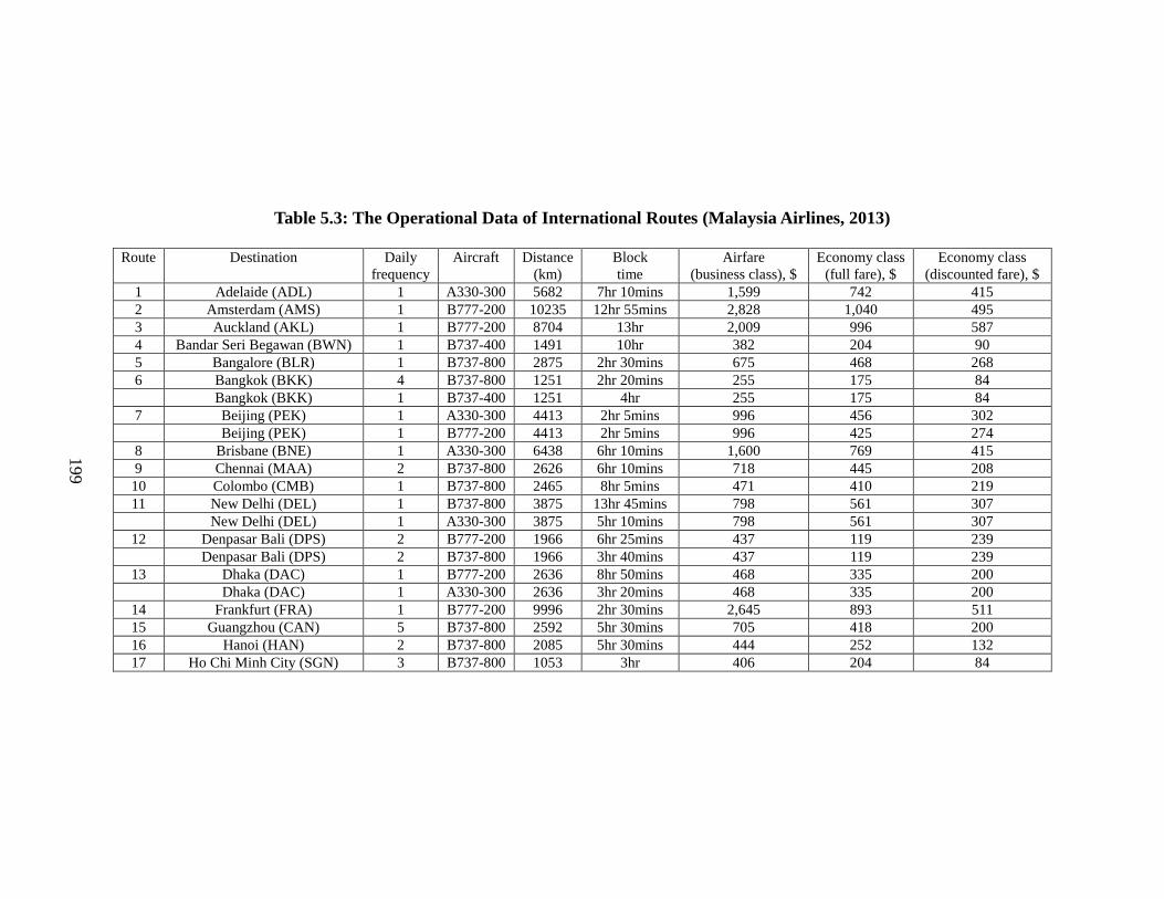
199

Table 5.3: The Operational Data of International Routes (Malaysia Airlines, 2013)

Route Destination Daily

frequency

Aircraft Distance

(km)

Block

time

Airfare

(business class), $

Economy class

(full fare), $

Economy class

(discounted fare), $

1 Adelaide (ADL) 1 A330-300 5682 7hr 10mins 1,599 742 415

2 Amsterdam (AMS) 1 B777-200 10235 12hr 55mins 2,828 1,040 495

3 Auckland (AKL) 1 B777-200 8704 13hr 2,009 996 587

4 Bandar Seri Begawan (BWN) 1 B737-400 1491 10hr 382 204 90

5 Bangalore (BLR) 1 B737-800 2875 2hr 30mins 675 468 268

6 Bangkok (BKK) 4 B737-800 1251 2hr 20mins 255 175 84

Bangkok (BKK) 1 B737-400 1251 4hr 255 175 84

7 Beijing (PEK) 1 A330-300 4413 2hr 5mins 996 456 302

Beijing (PEK) 1 B777-200 4413 2hr 5mins 996 425 274

8 Brisbane (BNE) 1 A330-300 6438 6hr 10mins 1,600 769 415

9 Chennai (MAA) 2 B737-800 2626 6hr 10mins 718 445 208

10 Colombo (CMB) 1 B737-800 2465 8hr 5mins 471 410 219

11 New Delhi (DEL) 1 B737-800 3875 13hr 45mins 798 561 307

New Delhi (DEL) 1 A330-300 3875 5hr 10mins 798 561 307

12 Denpasar Bali (DPS) 2 B777-200 1966 6hr 25mins 437 119 239

Denpasar Bali (DPS) 2 B737-800 1966 3hr 40mins 437 119 239

13 Dhaka (DAC) 1 B777-200 2636 8hr 50mins 468 335 200

Dhaka (DAC) 1 A330-300 2636 3hr 20mins 468 335 200

14 Frankfurt (FRA) 1 B777-200 9996 2hr 30mins 2,645 893 511

15 Guangzhou (CAN) 5 B737-800 2592 5hr 30mins 705 418 200

16 Hanoi (HAN) 2 B737-800 2085 5hr 30mins 444 252 132

17 Ho Chi Minh City (SGN) 3 B737-800 1053 3hr 406 204 84

199

200

Table 5.3 continued: The Operational Data of International Routes (Malaysia Airlines, 2013)

Route Destination Daily

frequency

Aircraft Distance

(km)

Block

time

Airfare

(business class), $

Economy class

(full fare), $

Economy class

(discounted fare), $

18 Hong Kong (HKG) 1 A380 2562 3hr 692 316 170

Hong Kong (HKG) 2 B737-800 2562 3hr 50mins 692 316 170

19 Hyderabad (HYD) 1 B737-800 3009 3hr 50mins 745 508 308

20 Jakarta (CGK) 6 B737-800 1141 12hr 41mins 697 455 64

21 Jeddah (JED) 1 B777-200 7055 9hr 10mins 971 762 489

22 Tribhuvan (KTM) 1 B737-800 3275 14hr 45mins 486 349 288

23 Kunming (KMG) 1 B737-800 2476 14hr 30mins 683 369 151

24 London (LHR) 2 A380 10603 4hr 5mins 2,911 1,248 549

25 Male (MLE) 1 B737-800 3133 5hr 15mins 959 463 318

26 Manila (MNL) 4 B737-800 2496 3hr 25mins 455 335 172

27 Melbourne (MEL) 1 A330-300 6329 15hr 30mins 1,462 583 283

28 Mumbai (BOM) 1 B737-800 3623 15hr 30mins 798 561 307

29 Osaka Kansai (KIX) 1 A330-300 4983 1hr 55mins 1,288 592 265

30 Paris (CDG) 1 A380 10439 3hr 50mins 2,518 924 460

31 Perth (PER) 1 A330-300 4139 3hr 50mins 1,267 636 254

32 Phnom Penh (PNH) 2 B737-800 1040 4hr 10mins 419 192 70

33 Seoul Incheon (ICN) 1 A330-300 4606 2hr 1,127 267 558

34 Shanghai Pu Dong (PVG) 2 A330-300 3798 9hr 15mins 774 439 267

35 Taipei (TPE) 4 B737-800 3268 4hr 50mins 518 389 226

36 Tokyo Narita (NRT) 2 B777-200 5406 3hr 40mins 1,328 642 387

37 Xiamen (XME) 1 B737-800 2991 2hr 45mins 603 439 248

38 Yangon (RGN) 2 B737-800 1682 2hr 45mins 437 235 61

200

201

Table 5.4: The Expected Value of Flight Fare and Cost per Flight

Fare & Cost, $ Year 1 Year 2 Year 3 Year 4 Year 5 Year 6 Year 7 Year 8

1S

tE fare 124,122 136,534 150,188 165,207 181,727 199,900 219,890 241,879

2S

tE fare 117,916 129,708 142,678 156,946 172,641 189,905 208,895 229,785

3s

tE fare 111,710 122,881 135,169 148,686 163,554 179,910 197,901 217,691

1cosS

tE t 74,473 81,921 90,113 99,124 109,036 119,940 131,934 145,127

2cosS

tE t 70,750 77,825 85,607 94,168 103,585 113,943 125,337 137,871

3cosS

tE t 67,026 73,729 81,101 89,212 98,133 107,946 118,741 130,615

Table 5.5: The Purchase Cost, Lease Cost and Depreciation Cost of Aircraft

($ million)

Aircraft B737-400 B737-800 B777-200 A330-300 A380

Purchase cost 4.5 90.5 278.8 239.4 403.9

Lease cost 4.1 81.45 250.9 215.5 363.5

Depreciation cost

- purchased aircraft

- leased aircraft

0.8

0.7

16.3

14.7

50.2

45.2

43.1

38.8

72.7

65.4

Table 5.6: The Resale Price and Residual Value of Aircraft ($ million)

Year, y B737-400 B737-800 B777-200 A330-300 A380

1 3.7 74.2 228.6 196.3 331.2

2 2.9 57.9 178.4 153.2 258.5

3 2.1 41.6 128.2 110.1 185.8

4 1.3 25.3 78.1 67.0 113.1

5 0.5 9.1 27.9 23.9 40.4

Table 5.7: The Standard Operations Hour of Aircraft at Airport

(Boeing, 2013)

Airport Start of working hours End of working hours

Amsterdam (AMS) 6.00am 10.00pm

Frankurt (FRA) 6.00am 10.00pm

London (LHR) 6.00am 11.30pm

Paris (CDG) 6.00am 11.30pm

Kuala Lumpur (KLIA) 6.00am 11.30pm

In addition to the aforementioned data, other data input of the case

study are listed as follows:

202

By definition:

Three probable phenomenon, i.e. 3k are considered

Discount rate, %5t

r

Load factor, ,

70%i

t

n FLF




Annual aircraft availability, , i

t

n FAVT = 340 days

Portion of passenger in business class, % 12% Biz

Portion of passenger in economy class (full fare), % 20%Fec

Portion of passenger in economy class (discounted fare), % 80%Dec

11 and 1 for 1,..., ; 1k ks ss

t t t tD D D D t T k (5.25)

By assumption:

The probability to possess aircraft is 1 2

0 50, 0 36s sp . p . and

3 0.14sp

At 1t , initial quantity of aircraft to be four years old is

1 4 2 for 1,2,3,4P

iI i

Setup cost, 0ti

u

Maximum utilization of aircraft, ,1.05 actual aircraft utilization

t FiMXU

Airline's willingness to pay,

$6 millioniFW


Slot price, $5 millioniFC

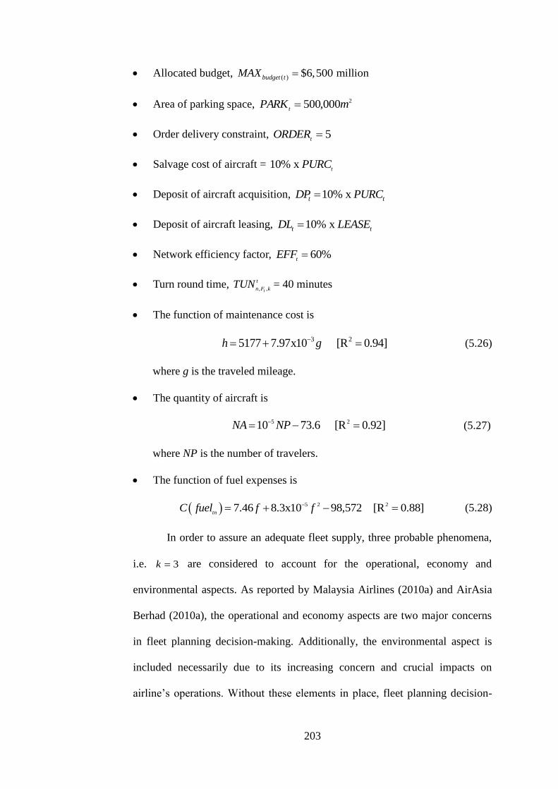
203

Allocated budget, ( ) $6,500 millionbudget tMAX

Area of parking space, 2000,500 mPARKt


ORDER

Salvage cost of aircraft = 10% x t

PURC

Deposit of aircraft acquisition, 10% x t tDP PURC

Deposit of aircraft leasing, 10% x t tDL LEASE

Network efficiency factor, %60t

EFF

Turn round time, , ,i

t

n F kTUN = 40 minutes


3 25177 7.97x10 [R 0.94]h g (5.26)

where g is the traveled mileage.


5 210 73.6 [R 0.92]NA NP (5.27)



5 2 27.46 8.3x10 98,572 [R 0.88]tn

C fuel f f (5.28)

In order to assure an adequate fleet supply, three probable phenomena,

i.e. 3k are considered to account for the operational, economy and

environmental aspects. As reported by Malaysia Airlines (2010a) and AirAsia

Berhad (2010a), the operational and economy aspects are two major concerns

in fleet planning decision-making. Additionally, the environmental aspect is

included necessarily due to its increasing concern and crucial impacts on

airline‟s operations. Without these elements in place, fleet planning decision-

204

making may not be suitable to support the operating networks under

uncertainty. Based on the reports of Malaysia Airlines (2010a) and AirAsia

Berhad (2010a), Equations (5.26)-(5.28) are obtained by conducting

polynomial regression analysis (Meyer and Krueger, 2005). Equation (5.26)

signifies that a unit cost of 0.00797 is charged as maintenance cost for each

additional unit of mileage traveled. For this equation, $5177 indicates an

overall estimated maintenance cost without considering additional traveled

mileage. Besides, the regression analysis exhibits that Equation (5.27) is best

fitted as a linear function in terms of the number of travelers. Equation (5.27)

displays that every addition of 100,000 travelers requires one additional aircraft

for which the constant in Equation (5.27) has no practical interpretation.

Similarly, the analysis reveals that fuel expenses (Equation (5.28)) is best fitted

as a quadratic function in terms of the number of flights.

In order to investigate the impact of changes of the inputs to the

computational results, an additional scenario (without slot purchase), i.e.

scenario A is tested. By doing this, some differences compared to benchmark

scenario (with slot purchase) in making the optimal fleet planning decision

could be observed. The benefits of considering slot purchase could also be

identified. Besides, the connections of slot purchase, service frequency and

fleet planning of airlines could be captured. In addition, scenario B is examined

to inspect the impacts of optimal slot purchase decision in providing the

desired service frequency for new operating network (instead of adding service

frequency for existing operating networks). Specifically, scenario B is outlined

205

for airline's consideration to operate a new operating network for short-haul

route (labeled as #1), medium-haul rote (denoted as #2) and long-haul route

(indicated as #3). For new network expansion, the estimated demand level and

expected airfare of each operating route are shown in Table 5.8.

Table 5.8: The Estimated Demand Level and Average Fare for New

Network Expansion

Route Flight

type

Estimated

demand level

(per annum)

Airfare ($)

Business

class

Economy class

(full fare)

Economy class

(discounted fare)

#1 Short-haul 84,539 737 369 208

#2 Medium-haul 77,228 1680 840 474

#3 Long-haul 131,636 2,426 1,213 685 Note: The data input for new network expansion was compiled accordingly based on the average value of

existing operating networks (38 operating routes).

5.6 Results and Discussions

As mentioned earlier, slot purchase decision-making is determined

based on the optimal revenue of the individual operating period. It was found

that the long-haul flight from KL to London (KL-London) emerges as the most

gainful operating route (with maximum revenue). By making slot purchase

decision for this route (KL-London), the results of the developed two-stage

fleet planning decision model are displayed in Table 5.9. Table 5.9 also shows

the results of scenario A which excludes the slot purchase in fleet planning and

scenario B for new network expansion. The relevant graphical results are

displayed in Figure 5.2.

206

Table 5.9: The Computational Results of Respective Scenario

Benchmark scenario Scenario A Scenario B

Slot purchase consideration Yes No Yes

Slot purchase decision for existing networks (Yes implies slot purchase is made;

No indicates no slot purchase)

Yes: Year 1,2,4,6,7,8 No: Year 3,5

Nil Yes: Year 2,4,6,7,8 No: Year 3,5

Slot purchase decision for new network Nil Nil Yes: Year 1 No: Year 2-8

Revenue and profit

Annual revenue (contributed by slot purchase), $

- existing network - new network

33,912,947 Nil

Nil Nil

33,912,947 129,917,782

Annual profit of airline, $ 579,890,573 555,565,392 784,890,573

Demand

Annual demand (met by slot purchase)

- existing network - new network

29,045 Nil

Nil Nil

29,045 131,636

Average demand level of airline 8,944,533 8,934,261 9,076,169

Service frequency

Annual service frequency (provided by slot purchase) - existing network

- new network

42

Nil

Nil

Nil

42

251

Average service frequency of airline (per annum) 27,864 27,832 28,115

Fleet Planning Decision

Fleet size (at the end of the planning horizon) 55 54 57

B737-400 18 18 18

B737-800 16 16 16

B777-200 6 6 6

A330-300 12 12 12

A380 3 2 5

Quantity of purchased aircraft: leased aircraft 48:7 50:4 48:9

Ratio of purchased aircraft: leased aircraft 87%:13% 93%:7% 84%:16%

Figure 5.2: The Graphical Results of Two-Stage Fleet Planning Decision

Model

207

As shown in Table 5.9, the benchmark scenario (with slot purchase

decision) provides a higher service frequency, i.e. 27,864 which is 42 times

more than scenario A (without slot purchase). Correspondingly, the demand

level met by the benchmark scenario appears to be higher in average, i.e. it is

approximately to be 10,272 more than scenario A (per annum). This signifies

that the airline could meet a higher level of stochastic demand by providing

more service frequency via optimal slot purchase decision. This finding is in

line with the facts as revealed by Brueckner (2009), Fukui (2010) and Babic

and Kalic (2011, 2012). Consequently, more profit could be obtained by airline

due to the contribution of a higher level of revenue which is mainly generated

by additional flights (resulted from slot purchase decision of KL-London). This

shows that by making an optimal slot purchase decision, a higher demand level

could be met by airlines at a more profitable level. On average, it is

approximated that an additional 1% of demand increment that is met via slot

purchase decision would constitute about 0.97% of service frequency (flight).

This is coherent with the findings of Pitfield et al. (2009) who revealed that the

demand increment would increase service frequency. Such increment would

then result in additional revenue at $2.88 million (average value per annum),

which consequently contributes about $6.15 million of profit (per annum).

Similar fact also shows that slot purchase is useful for airlines to assure that

more profit could be seen in Babic and Kalic (2011, 2012).

Specifically, Table 5.9 shows that airline did not make any slot purchase

decision for operating year 3 and 5 (for benchmark scenario). This could be

208

explained by the level of stochastic demand that is estimated to drop about

32% in year 3 (see Table 5.2). For year 5, there is no demand increment

(compared to previous year, i.e. year 4) and hence slot purchase decision did

not apply for these operating periods. Under these circumstances, the airline

may consider to sell or lease the slot to other airlines for additional income

(Fukui, 2010). This shows that the developed model is able to provide

insightful information to airlines at the right time to make relevant slot

purchase decision throughout long-term planning horizon.

In order to provide a higher service frequency (via slot purchase

decision) to meet demand increment, the results (in Table 5.9) show that airline

would tend to acquire/lease more aircraft to support the current operating

network. As shown in Table 5.9, benchmark scenario, which includes slot

purchase decision, possesses one more aircraft, i.e. A380, compared to scenario

A which does not account for slot purchase decision. In accordance to slot

purchase decision to service the KL-London route, A380 is leased mainly due

to their availability in supporting long-haul flight (KL-London) at a more

economical aircraft acquisition/lease cost per seat. This signifies that there is a

positive relation between the slot purchase decision and fleet planning decision

of airlines for which the slot purchase decision-making that basically aims to

provide a higher service frequency to meet more demand would practically

require more aircraft (via acquisition/leasing) for services. Yet, the optimal

quantity of respective aircraft type that is needed for additional operations is

very much dependent on the operating route and corresponding demand level

209

that is to be serviced via slot purchase, e.g. the KL-London route would require

jumbo aircraft (A380). Conversely, it could be inferred that there is a tendency

for airlines to acquire/lease fewer aircraft if the slot purchase decision is not

taken into consideration (as shown by the fleet size of scenario A). Besides, the

results show that airline tends to lease aircraft rather than purchase new aircraft

when slot purchase is incorporated in fleet planning. This could be justified by

the cost of aircraft leasing which is much lower than aircraft purchase cost and

hence aircraft leasing is preferred in fleet planning in order to assure a higher

profit of airline. This explains that the portion of leased aircraft of benchmark

scenario (with slot purchase) which appears to be much higher than scenario A

(in Table 5.9).

Apparently, it could be empirically deduced that demand increment

influences the slot purchase decision positively and it is observable that slot

purchase has a positive impact on service frequency, fleet supply as well as

profit level. This shows that slot purchase has a direct and closed linkage not

only with the demand aspect but also the supply aspect, which are relatively

vital for the supply-demand management. More importantly, the results show

that the incorporation of slot purchase in fleet planning is beneficial to airlines

in achieving social and economic sustainability. This is practically viable for

airlines by providing a better service quality via a higher service frequency to

meet more demand (social aspect) as well as obtaining a higher revenue and

profit (economic aspect) by making optimal slot purchase and fleet planning

decision.

210

5.6.1 Further Application: New Network Expansion

In view of the benefits of optimal slot purchase decision in meeting

more demand via a higher service frequency (as discussed earlier), the

developed model could also be adopted suitably to expand new network (see

Appendix C for more details about the model modification). It is anticipated

that the new network expansion which would provide additional (new) service

frequency would generate additional revenue and profit to airlines. By

considering three new networks (for scenario B), i.e. #1 (short-haul), #2

(medium-haul) and #3 (long-haul), the developed SPDM (stage 1) shows that

long-haul route (#3) generates the highest revenue compared to other routes.

This suggests to the airline to operate new operating network, i.e. #3 (at the

beginning of operating period 1) and this would contribute a total of 39

operating routes, in overall, throughout the planning horizon. Besides, the

results of scenario B show that new network expansion (via optimal slot

purchase and fleet planning decision) would be able to meet a higher level of

demand which is approximately 131,636 more than the benchmark scenario

(per annum). Correspondingly, scenario B would provide an additional of 251

flights (service frequency) per annum to meet increasing demand (for new

network #3). This would then contribute more revenue to airline, i.e. $130

millions (from new network) and consequently generate more annual profit, i.e.

approximately to be $785 million per annum.

211

In terms of the fleet size (compared to benchmark scenario), the

findings in Table 5.9 show that airline would possess more aircraft (via aircraft

leasing) for new network expansion. For aircraft leasing, two A380 is chosen

optimally not only due to its technical specification in supporting the long-haul

network (#3), but also to assure optimal profit of airline. In overall, the findings

produced by the developed model show that new network expansion (with

optimal slot purchase and fleet planning decision) yields beneficial returns to

airlines in meeting more demand (with a larger fleet composition for desired

service frequency) as well as producing higher profit margin.

5.6.2 Results Verification

The consistency and stability of computational results could be

empirically confirmed by comparing the findings with actual operational

statistics of airline (Malaysia Airlines, 2013). Table 5.10 summarizes the fleet

size of airline (i.e. MAS) as compiled from accessible annual reports and

optimal fleet planning decision of each operating period as obtained from the

developed model. It could be observed that the fleet size of MAS during

operating years of 2006 to 2012 falls within the range of two standard

deviations from its average. The optimal solutions obtained from the

benchmark problem, scenarios A and B show similar pattern, i.e. the fleet size

of operating periods 1 to 8 falls within the range of two standard deviations

from its average. Similar pattern could be observed from Table 5.11 for service

212

frequency determination of airline. Therefore, it is apparent that the solutions

obtained from the developed model are coherent with the operating

performance of airline. As such, the findings are consistent with the actual

practice and hence the stability of the results (as well as the developed model)

could be empirically confirmed.

Table 5.10: The Summary of Fleet Planning Decision

Empirical report Scenario

Year MAS* t Benchmark A B

Operating period (Note for *: The fleet size of MAS

are computed only for

international network, which is approximated to be 35% of total

operating networks (Malaysia

Airlines, 2013))

2005 39 1 48 48 50

2006 34 2 44 43 45

2007 36 3 44 43 45

2008 38 4 46 44 47

2009 39 5 46 44 47

2010 41 6 49 46 50

2011 45 7 52 48 53

2012 50 8 55 49 57

Average (AG) 40.3 48.0 45.6 49.3

Standard Deviation (SD) 5.1 3.9 2.4 4.2

AG + 2SD 50.5 55.8 50.5 57.6

AG – 2SD 30.0 40.2 40.7 40.9

Table 5.11: The Summary of Service Frequency of Airline

Empirical report Scenario

Year MAS* Benchmark A B

Operating period (Note for *: The service frequency

of MAS are computed only for international network, which is

approximated to be 35% of total

operating networks (Malaysia Airlines, 2013))

2005 51,634 1 30,175 30,123 30,426

2006 53,719 2 31,635 31,583 31,886

2007 43,021 3 24,556 24,556 24,807

2008 39,640 4 26,191 26,166 26,442

2009 37,486 5 26,091 26,091 26,342

2010 42,795 6 26,971 26,929 27,222

2011 38,071 7 27,814 27,768 28,065

2012 36,777 8 29,482 29,445 29,733

Average (AG) 42,893 27,864 27,833 28,115

Standard Deviation (SD) 6,482 2,386 2,369 2,386

AG + 2SD 55,857 32,637 32,570 32,888

AG – 2SD 29,929 23,092 23,095 23,343

213

5.7 Summary

This research developed a novel methodology to solve the long-term

fleet planning problem under stochastic demand. A two-stage fleet planning

decision model is formulated for which the aim of the first stage is to select

individual operating route (at optimal revenue) that necessitates the slot

purchase to meet demand increment while the second stage aims to maximize

the operational profit of airlines, by determining the optimal quantity of

respective aircraft type (with corresponding service frequency) that is to be

purchased and/or leased. The results of a realistic case study with 38

international routes demonstrated that the developed methodology is sensitive

to the modeling parameters and it is feasible in providing optimal solutions for

fleet planning problem. Concisely, the findings revealed that slot purchase is

beneficial to airlines in assuring a higher profit level. This could be achieved

when a higher level of travel demand is met by providing more service

frequency (with optimal slot purchase decision). By incorporating slot purchase

in fleet planning, it was also found that airline would tend to lease aircraft

rather than purchase new aircraft, yet the quantity and aircraft type is

dependent on specific operating route that requires slot purchase. The

developed methodology, in fact, reflects realistically the actual situation of

airline industry, ranging from the challenges of providing the desired service

frequency (by incorporating slot purchase) to meet stochastic demand under

uncertainty to the practical issues in acquiring/leasing adequate fleet supply

under numerous practical constraints.

214

CHAPTER 6

ENVIRONMENTAL PERFORMANCE ASSESSMENT FOR FLEET

PLANNING

6.1 The Role of Environmental Performance Assessment

In response to environmental concern which is receiving greater

attention nowadays by the airlines industry, airlines play a vital role in

conserving the environment. Ideally, airlines should reduce the amount of

pollutants emitted from their operating networks. Specifically, three major

environmental factors of airlines, namely aircraft emission, noise and fuel

consumption, could be decreased at a larger scale by having a well-defined

monitoring system. As such, a modeling framework of green index is

formulated to assess the environmental (green) performance of airlines. The

developed framework is able to quantify airline's green level of aircraft

emission, noise and fuel efficiency specifically based on the aircraft operations

of airlines in supporting the current operating networks. Subsequently, the

overall green performance of airlines in terms of Green Fleet Index (GFI) could

then be compiled systematically. The resultant GFI, as a green indicator, is

capable to reveal not only the green performance of airlines at present, but also

provide some constructive improvement strategies to yield a greener

performance. The effectiveness of the respective improvement strategy could

also be identified accordingly for airline's further action. The formulations of

215

the respective green level (for aircraft emission, noise and fuel efficiency) as

well as the GFI of airlines are outlined in following sections. The applicability

of the developed modeling framework is tested with an illustrative case study.

The results show that the developed methodology is practically feasible to

assist airlines to achieve a greener performance.

6.2 Quantify Green Index: Gini Coefficient

Basically, Green Index (GI) measures the degree of environmental

performance, i.e. it is an environmental indicator which signifies the scale of

green performance based on the aircraft operations of airlines. The GI is

derived borrowing the concept of Gini coefficient (Gini, 1912), which is

originally created to reflect the income distribution of a nation‟s residents. It is

a measure of statistical dispersion which indicates the inequality among the

values of a frequency distribution. The coefficient that ranges from zero

(minimum) to one (maximum) indicates the equality degree from perfect

equality to imperfect equality. Geometrically, the Gini coefficient is expressed

as a ratio of two regions defined by a 45 degrees line (i.e. the line of perfect

equality) and a Lorenz curve. The area of region under the Lorenz curve can be

evaluated based on the properties of trapezoid whereas the area under the line

of perfect equality is exactly half in a unit box. Gini coefficient can also be

computed using the mean difference formula, covariance approach and matrix

form. Despite different formulations with its own appeal in a specific context,

216

the formulations are mathematically equivalent (Xu, 2004).

In view of the fact that Gini coefficient measures the equality degree

(with the scale from zero to one), this signifies that a data set that is closer to

each other (by having a narrower gap) would tend to have a lower Gini

coefficient, and vice versa. In other words, a data set with a higher equality

would tend to have a smaller variance or standard deviation (due to a narrower

gap among the data). This reveals that a smaller variance or standard variance,

in fact, could reflect a greener performance. As such, if airlines could reduce

their aircraft emission, noise and fuel consumption effectively (especially for

specific operating route with critical pollutants or fuel consumption), the

resultant operating networks would produce a lesser amount of pollutants and

hence a smaller variance or standard deviation could be obtained (by having a

smaller average too). Equivalently, a greener performance by airlines would

have a lower Gini coefficient, average, variance as well as standard deviation.

As such, Gini coefficient is adopted to quantify the green level of airlines.

Practically, a greener performance could be achieved if airlines could

implement some improvement strategies effectively.

In this research, the GI is computed by using the geometrical approach

as shown in Equations (6.1) and (6.2):

2GI A (6.1)

where the component of A indicates the area in between the Lorenz curve

217

and the line of perfect equality. It is evaluated as follows:

1 1

1 1

2 2c c c c

c

A W W Cat Cat

(6.2)

for which cW indicates the cumulative percentage of environmental factor W

(for the vertical axis) while cCat

denotes the cumulative percentage of

operating routes (for the horizontal axis) in category c. Category, c, refers to

the group of environmental factor (with the corresponding operating routes)

ranked in ascending order. Fellman (2012) pointed out that the simplest way is

to define five quintiles or 10 deciles for Lorenz curve, i.e. 5 ,4 ,3 ,2 ,1c for

five quintiles and 10 ,...,2 ,1c for 10 deciles. For the right hand side of

Equation (6.2), the constant of half refers to the area under the line of perfect

equality while second component denotes the total area under the Lorenz curve

(based on the properties of trapezoid). Alternatively, the GI can be simplified as

follows:

1 11 c c c c

c

GI W W Cat Cat

(6.3)

Mathematically, 0GI indicates that the environmental performance of

airlines, in overall, is greener while 1GI implies that the green performance

of airlines is getting poorer and exhibits a greater tendency to be not green for

the current operating networks. Specifically, greener performance implies that

there is a lesser amount of emission, noise and/or fuel consumption produced

from aircraft operations of a particular operating year (in comparison to

previous year). In order to quantify the overall environmental performance of

airlines of a particular operating period, three indices are derived specifically

for aircraft emission, noise, and fuel consumption (as explained below).

218

6.2.1 Green Emission Index

The relevant contributing factors to aircraft emission are load factor,

aircraft status (new or aging), emission rate and service frequency. Aircraft

emission is computed during landing and take-off (LTO) cycle as well as

cruising stage. In fact, emission produced from LTO and cruising stages are

reported to be different. According to Givoni and Rietveld (2010), the resultant

emission from LTO stage is found to be harmful as local air pollution while

aircraft emission from the cruising stage would result in climate change issues.

The aircraft emission rate, which is contributed by hydrocarbon (HC), carbon

monoxide (CO), particular matter (PM), nitrogen oxides ( xNO ) and sulphur

oxides ( 2SO ), i.e. major elements produced from LTO and cruising stages,

measured for each aircraft in kilogram. Miyoshi and Mason (2009) and Chao

(2014) revealed that both LTO and cruising stages have to be considered to

capture aircraft emission completely. As such, the total aircraft emission of

airlines of a particular operating year t , tEX , can be expressed in general form

as follows:

2

, ,

1

, , 1

,

, , 1,..., ; 1,..., ; ,...,

i i

i

i i

i

t i S i

t i F t i F t t

F

t i S i

i F t i F t t k

F

EX LF ER f D A OLD

LF ER f D A NEW t T i n S s s

(6.4)

where , i

t

n FLF refers to load factor, n

tER is the emission rate of individual flight

(depending on aircraft type), , ,i

m S n

n F t tf D A

is the service frequency of

operating route (depending on the level of travel demand, tD and total quantity

219

of aircraft, tA of airline which may vary for different status of aircraft, m for

which 1m refers to new aircraft while 2m

implies aging aircraft,

is the

parameter of environmental sustainability while OLD and NEW

respectively

indicates the proportion of aging (more than 1 year old) and new (up to 1 year

old) aircraft that servicing route OD. Particularly, total quantity of aircraft

refers to total number of fleet (aircraft) in operation for which airline's fleet

supply is obtained by making optimal aircraft acquisition/leasing decision.

According to Grampella et al. (2013), the respective aircraft type with

different engines was found to emit pollutants differently and hence they used

engine-weighted pollutants to compute aircraft emission level. In order to

compute the total emission level of airlines of a particular operating period, in

fact the developed Equation (6.4) could be applied similarly to capture engine-

weighted pollutants for which a particular amount of pollutants (engine-

weighted) can be compiled in terms of the emission rate of a specific aircraft

type. Specifically, Equation (6.4) is formulated to compute the total aircraft

emission of the landing and take-off (LTO) and cruising stages, i.e. the entire

aircraft operation (with weighted-amount of pollutants) is taken into

consideration completely. Particularly for the LTO stage, the engine-weighted

emission rate of hydrocarbon (HC), carbon monoxide (CO), particular matter

(PM), nitrogen oxides (NOx) and sulphur oxides (SO2) can be compiled

accordingly to determine the total amount of emission level of each pollutant

(for the respective aircraft type).

220

The EGI is then computed by using the following equation:

, , 1 11 , 1,...,E t c t c c c

c

GI EX EX Cat Cat t T

(6.5)

for which ,t cEX

and

cCat

respectively denotes cumulative percentage of

emission level (for vertical axis) and operating routes (for horizontal axis) in

category c. Mathematically, 0EGI signifies that the environmental

performance of airlines in terms of aircraft emission appears to be better and

greener for which, in overall, the servicing routes in current operating network

produce a lesser amount of emission. On the other hand, 1EGI implies that

the green performance of airlines is getting poorer and exhibits a greater

tendency to be not green for current operating networks. This could happen

when the operating routes emit exceptional high amount of aircraft emission.

Such a substantial aircraft emission from the operating networks would

negatively affect the overall green performance of airlines.

6.2.2 Green Noise Index

Generally, the level of aircraft noise of a particular flight can be

computed based on three reference points, namely stage of lateral ( Lf ),

approach ( Af ) and flyover ( F

f ) (ICAO, 2011). According to ICAO (2011),

aircraft noise level during these stages is greatly affected by aircraft weight

(closely related to load factor) and number of engines of aircraft. Accordingly,

the cumulative noise level, tEXN , of a particular operating year, t of airlines

221

can be generalized as follows:

2

, ,

1

, , 1

, ,

, , , 1,..., ; 1,..., ; ,...,

i i

i

i i

i

t S i

t i F L A F i F t t

F

t S i

i F L A F i F t t k

F

EXN LF f M f M f M E f D A OLD

LF f M f M f M E f D A NEW t T i n S s s

(6.6)

where ( )Lf M , ( )Af M and ( , )Ff M E respectively represents aircraft noise

level at lateral, approach and flyover stages which greatly depends on aircraft

weight, M and number of engines, E. Note that annual cumulative noise level

of airlines is contributed by all servicing flights and hence the service

frequency of respective route, , ,i

m S n

n F t tf D A is included in Equation (6.6).

Besides, it is important to note that aging and new aircraft might emit different

noise level (mainly due to their technical specifications) and hence the status of

aircraft, m (i.e. 1m

for new aircraft and 2m

for aging aircraft) is

considered to compute cumulative noise level.

Specifically, Equation (6.6) is formulated to compute the cumulative

noise level of a particular operating year. The formulation of this equation is

guided by the three noise certification values (at the stages of lateral, approach

and flyover) of aircraft (ICAO, 2011). In practice, some airports are relatively

concern on the sum of the noise certification levels of aircraft (which

consequently determine the noise charges) and hence the sum of these stages

(at lateral, approach and flyover) is formulated accordingly in Equation (6.6).

Some of the examples of airport that impose noise charges by referring to the

sum of the noise certification levels of aircraft are Tokyo-Haneda airport,

222

Amsterdam-Schiphol airport and Sydney airport (Hsu and Lin, 2005). The

relevant study which make uses the sum of the three noise certification values

could be seen in Givoni and Rietveld (2010) for which they obtained the sum

value (of lateral, approach and flyover stages) and subsequently determine the

corresponding average in order to assess aircraft noise exposure level. This

shows that the three noise certification values can be summed up for further

computation. However, they considered only one aircraft type in their

formulation. In view of the fact that noise charges are airport-specific, it is

important to note that there are various formulas to determine the aircraft noise

level (with corresponding charges). The formula of energetic mean, which

could be seen in Adler et al. (2013), Martini et al. (2013) and Grampella et al.

(2013), was also found to be a useful approach and it is mainly used to

determine airport noise charges (for different noise level).

The NGI is then computed by using the following equation:

, , 1 11 , 1,...,N t c t c c c

c

GI EXN EXN Cat Cat t T

(6.7)

for which ,t cEXN

and

cCat respectively indicates cumulative percentage of

noise level (for vertical axis) and operating routes (for horizontal axis) in

category c. Basically, 0NGI implies that in terms of the environmental

performance of airlines, the green level of aircraft noise is getting better (with a

tendency to be quieter or greener) by producing lesser aircraft noise throughout

the planning horizon. Conversely, 1NGI signifies that the green level of

aircraft noise is getting worst (poorer or not green). This reveals that aircraft

223

noise is emitted substantially by servicing routes in the current operating

networks. Under this circumstance, an extensive level of aircraft noise would

affect and worsen the overall green performance of airlines.

6.2.3 Green Fuel Efficiency Index

An aircraft that is more fuel-efficient utilizes less fuel in servicing the

operating networks of airlines. Less fuel consumption by a particular fleet (e.g.

new aircraft) is relatively beneficial to airlines to travel further as well as to

meet a higher level of demand. Therefore, the total traveled mileage, travel

demand and fuel consumption are considered simultaneously to quantify the

green level of fuel efficiency. For a particular operating period t, the fuel

efficiency level, tFEL of airlines can be expressed as follows:

2

,

, 2 2

, ,

1

,

, 11 1

, ,

,

, ,

,

, 1,..., ; 1,..., ; ,...,, ,

i

i

i

i i

i i

i

i

i

i i

i i

S i

i F t t

Ft

t i F t S i S i

i F t t i F t t

F F

S i

i F t t

Ft

i F kS i S i

i F t t i F t t

F F

FC D A OLD

FEL LFgf D A NP D A

FC D A NEW

LF t T i n S s sgf D A NP D A

(6.8)

where , ,i

m S i

n F t tFC D A , , ,i

m S i

n F t tgf D A and , ,i

m S i

n F t tNP D A

respectively

denotes the fuel consumption, traveled mileage and total of passenger of

operating route iF . Note that 1 2

, ,, ,i i

i i

S i S i

i F t t i F t t

F F

FC D A FC D A

.

224

The FEGI is then computed by using the following equation:

, ,1 , 1,...,FE t c t c c c

c

GI FEL FEL Cat Cat t T

(6.9)

for which ,t cFEL

and

cCat respectively refers to cumulative percentage of fuel

efficiency level (for vertical axis) and operating routes (for horizontal axis) in

category c. Similar to the concept of the green level of aircraft emission and

noise, 0FEGI signifies that the environmental performance of airlines from

the aspect of fuel efficiency is getting better (and greener) with less fuel

consumption in overall to service the current operating networks. Conversely,

1FEGI denotes that the green level of airlines in terms of fuel efficiency

tends to be poorer and not green due to extensive fuel consumption in the

current operating networks. Such an operating system (with substantial fuel

consumption) would subsequently affect the green performance of airlines.

Compared to Equation (6.4) which calculates the total aircraft emission

of airlines, Equation (6.8) computes the total amount of fuel consumed by

airlines to support the entire operating networks. Note that in the case when

more fuels are consumed by airlines, there are more aircraft emissions emitted

to the environment. In other words, there is a direct linkage between fuel

consumption and aircraft emission as fuel consumption determines the amount

of emission proportionally. Contrary to aircraft emission, aircraft fuel does not

have direct impacts to the environment but aircraft emission emitted through

fuel burning would produce some harmful pollutants (e.g. carbon dioxide).

225

6.3 Quantify Green Fleet Index: Analytic Hierarchy Process

As displayed in Figure 6.1, by taking into consideration the Green

Index (GI) of W environmental factors (e.g., aircraft emission, noise and fuel

efficiency), the overall environmental performance of airlines in terms of

Green Fleet Index (GFI) can be quantified systematically by making use

Analytic Hierarchy Process (AHP) (Zadeh, 1965; Saaty, 1980). Owing to the

fact that the environmental performance of airlines is relatively influenced by

the occurrence of unexpected event which may affect the green performance of

airline, AHP which is capable to capture fuzziness or uncertainty (Zhü, 2014) is

adopted to quantify the GFI. For instance, heavy air traffic congestion (due to

demand increment) may affect the aircraft landing process at a particular

airport and this may result in more fuel consumption (and emission) due to the

unavailability of airport for landing. In such a case, fuel consumption (and

emission) of airlines may appear to be more significant relative to aircraft

noise. This highlights that by capturing the occurrence of unexpected event, the

resultant output of GFI would reflect the actual operations closely and the

green performance of airlines could be monitored in a better manner.

Recognizing the need to capture fuzziness in practice, AHP which is originated

from the fuzzy set theory was first introduced by Zadeh (1965) with the

attempt to select and prioritize a number of actions by evaluating a group of

predetermined criteria. The AHP is widely applied in other sectors, including

resource management and corporate strategy (Velasquez and Hester, 2013).

However, none of the literatures apply AHP to solve the environmental issue in

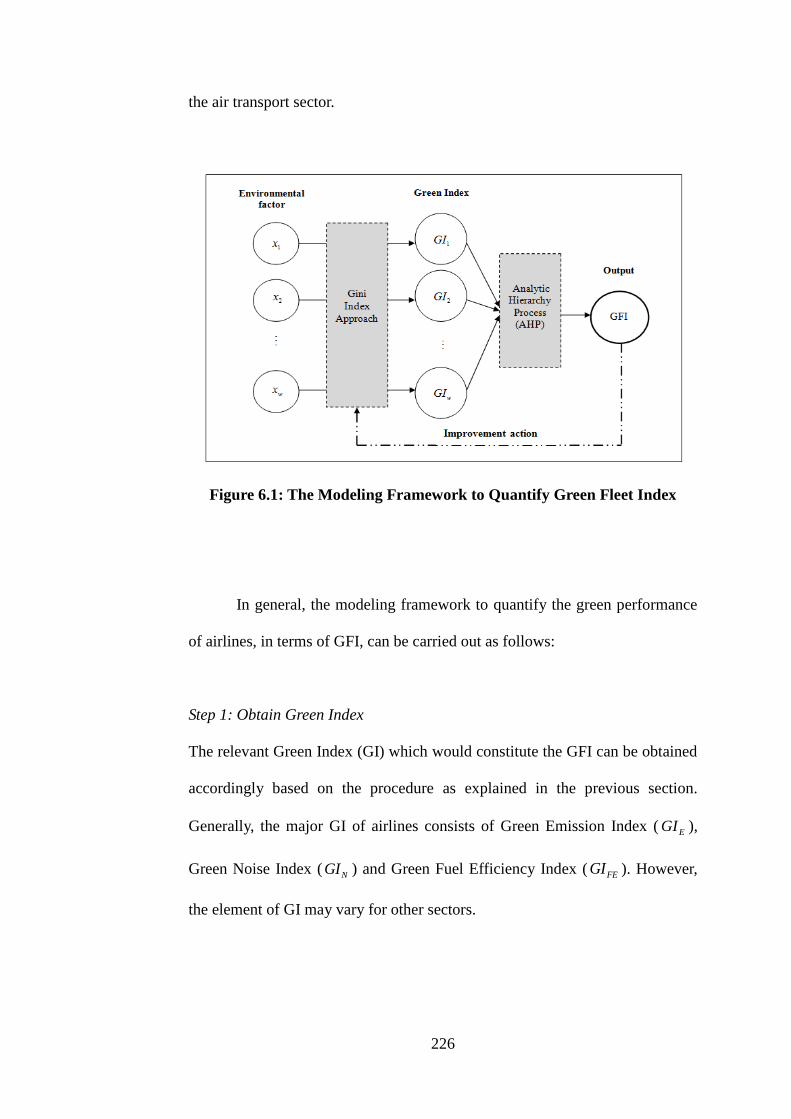
226

the air transport sector.

Figure 6.1: The Modeling Framework to Quantify Green Fleet Index

In general, the modeling framework to quantify the green performance

of airlines, in terms of GFI, can be carried out as follows:

Step 1: Obtain Green Index

The relevant Green Index (GI) which would constitute the GFI can be obtained

accordingly based on the procedure as explained in the previous section.

Generally, the major GI of airlines consists of Green Emission Index ( EGI ),

Green Noise Index ( NGI ) and Green Fuel Efficiency Index ( FEGI ). However,

the element of GI may vary for other sectors.

227

Step 2: Establish judgment matrix (for the relative comparison of GI)

A pair-wise comparison matrix, A involving the relative comparison of GI (as

obtained in step 1) can be expressed as follows (Saaty, 1980):

12 1

212

1 2 x

1

1 1

1 1 1

n

n

n n n n

a a

aa

A

a a

(6.10)

for which ij

a indicates relative comparison of green index i

GI over j

GI .

Generally, matrix A is governed by x , , ij jk ika a a i j k to assure

consistency. Specifically, ija implies the subjective judgment (relative

comparison) of criteria i over j based on judgment scale 1-9 (Saaty, 1977, 1980,

1990).

Step 3: Calculate the largest eigenvalue

As an indicator for consistency, the largest eigenvalue, max

of a matrix can be

determined as follows (Saaty, 1990):

max

, 1

nj

ij

i j i

wa

w

(6.11)

for which ija is the element of matrix A while

iw and

jw respectively

represent the average of row i and j of matrix A. Note that a matrix is said to be

more consistent if the value of the largest eigenvalue is getting closer to matrix

size.

228

Step 4: Perform consistency test

A consistency test is needed to assure the consistency of matrix A (with size n).

This test can be conducted based on the consistency index, CI and random

consistency index, RI which are outlined as follows (Saaty, 1977).

max1.98 2

, 1

nnCI RI

n n

(6.12)

Saaty (1977) showed that max n if the matrix does not include any

inconsistency. This implies that the closer the value of max to n, the matrix is

more consistent. By using the measurement of CI and RI, the consistency ratio,

CR can be evaluated as follows:

CI

CRRI

(6.13)

The judgment matrix is said to be consistent if CR < 0.1.

Step 5: Establish judgment matrix of green status (for each GI)

To capture the possible green status of GI that might be green or not green, a

pair-wise comparison matrix of each GI, WGI

B can be formed as follows:

2 2

1

1W

ij

GI

ji x

sB

s

(6.14)

for which matrix WGI

B is a square matrix with a size 2 x 2 while ijs reflects the

relative comparison of green status i

s over j

s . Green status basically

comprises two possible conditions (categories or status), i.e. green or not green.

In fact, there is no restriction for the number of status, Equation (6.14) could be

applied appropriately for more categories as desired by airlines.

229

Step 6: Perform consistency test

The consistency of matrix, WGI

B can be confirmed directly by checking

x , ,ij jk ika a a i j k . In fact, matrix of size 2 x 2 is indeed consistent in view

of the fact that 12 21 11 x =1 a a a .

Step 7: Compute the Green Fleet Index (GFI)

The resultant GFI can be evaluated as follows:

* *

i rGFI A B (6.15)

where *

iA represents the average of row 1, 2,...,i n of normalized matrix A

while *

rB denotes the average of row 1, 2,...,r a of normalized matrix WGI

B .

Note that a lower GFI value implies a greener performance.


A realistic example is set up to evaluate the applicability of the

developed methodology. In order to get closer to reality, most of the data used

for evaluation were obtained from accessible published reports. The data

resources include the websites of AirAsia Berhad (2013), Malaysia Airlines

(2013), Airbus (2013) and Boeing (2013).

230


It is assumed that an airline that is based at the Kuala Lumpur

International Airport (KLIA) is operating a total of 38 routes (as shown in

Table 6.1) with five types of aircraft, namely B737-400, B737-800, B777-200,

A330-300 and A380. These aircraft are chosen based on the fleet composition

operated by Malaysia Airlines (Malaysia Airlines, 2013) in servicing

international routes at 70% load factor (in average). In order to examine the

green performance of airline for a planning horizon of one year, the operations

of these aircraft are considered accordingly. The specification of aircraft

(including the fleet size of airline) and the environmental performance of

aircraft are shown in Tables 6.2 and 6.3, respectively while the annual travel

demand of airline, which is estimated to be 10,080,858 is obtained from the 5-

step demand modeling framework. Besides, the service frequency of airline,

i.e. 35,672 flights is compiled from the annual reports of airline (AirAsia

Berhad, 2013).

A do-nothing scenario is assessed by using the aforementioned data

input (without implementing any improvement action). In addition, four

improvement strategies, namely increase load factor (strategy A), operate new

aircraft (strategy B), reduce service frequency (strategy C), and reduce fuel

consumption (strategy D), as shown in Table 6.4, were evaluated to examine

their impact on the green performance of airlines. Although these improvement

231

strategies might be related to one another to a certain extent, it is important to

note that each strategy would be planned and implemented by airlines at a

different stage. Increasing load factor (strategy A) could be categorized as pre-

operational strategy for which airlines would need to carry out effective actions

to keep the load factor high. This could be done in numerous ways, including

implementing attractive marketing strategies to boost up flight ticket sales and

perform joint-efforts or alliances (if necessary) among airlines. Besides,

operating new aircraft (strategy B) could be considered as operational strategy

towards aircraft activities in servicing the current operating networks. For

strategy C, service frequency reduction refers to the strategy of airlines to

retain the same capacity of passengers by reducing the number of flights. This

is particularly required especially when airlines are controlled strictly under

capacity/runway constraints. One of the ways for airlines to retain the same

number of passengers is to operate a larger size of aircraft. For strategy D, fuel

consumption reduction could be done in several ways, especially during

aircraft operations. It is anticipated that airlines would have a greener

performance by consuming less fuel which produce fewer pollutants.

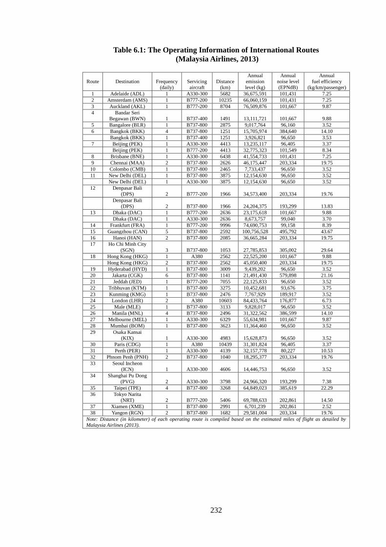
232

Table 6.1: The Operating Information of International Routes

(Malaysia Airlines, 2013)

Route

Destination

Frequency (daily)

Servicing aircraft

Distance (km)

Annual

emission level (kg)

Annual

noise level (EPNdB)

Annual

fuel efficiency (kg/km/passenger)

1 Adelaide (ADL) 1 A330-300 5682 36,675,591 101,431 7.25

2 Amsterdam (AMS) 1 B777-200 10235 66,060,159 101,431 7.25

3 Auckland (AKL) 1 B777-200 8704 76,509,876 101,667 9.87

4

Bandar Seri Begawan (BWN) 1 B737-400 1491 13,111,721 101,667 9.88

5 Bangalore (BLR) 1 B737-800 2875 9,017,764 96,160 3.52

6 Bangkok (BKK) 4 B737-800 1251 15,705,974 384,640 14.10

Bangkok (BKK) 1 B737-400 1251 3,926,821 96,650 3.53

7 Beijing (PEK) 1 A330-300 4413 13,235,117 96,405 3.37

Beijing (PEK) 1 B777-200 4413 32,775,323 101,549 8.34

8 Brisbane (BNE) 1 A330-300 6438 41,554,733 101,431 7.25

9 Chennai (MAA) 2 B737-800 2626 46,175,447 203,334 19.75

10 Colombo (CMB) 1 B737-800 2465 7,733,437 96,650 3.52

11 New Delhi (DEL) 1 B737-800 3875 12,154,630 96,650 3.52

New Delhi (DEL) 1 A330-300 3875 12,154,630 96,650 3.52

12

Denpasar Bali

(DPS) 2 B777-200 1966 34,573,400 203,334 19.76

Denpasar Bali

(DPS) 2 B737-800 1966 24,204,375 193,299 13.83

13 Dhaka (DAC) 1 B777-200 2636 23,175,618 101,667 9.88

Dhaka (DAC) 1 A330-300 2636 8,673,757 99,040 3.70

14 Frankfurt (FRA) 1 B777-200 9996 74,690,753 99,158 8.39

15 Guangzhou (CAN) 5 B737-800 2592 100,756,528 495,792 43.67

16 Hanoi (HAN) 2 B737-800 2085 36,665,284 203,334 19.75

17

Ho Chi Minh City

(SGN) 3 B737-800 1053 27,785,853 305,002 29.64

18 Hong Kong (HKG) 1 A380 2562 22,525,200 101,667 9.88

Hong Kong (HKG) 2 B737-800 2562 45,050,400 203,334 19.75

19 Hyderabad (HYD) 1 B737-800 3009 9,439,202 96,650 3.52

20 Jakarta (CGK) 6 B737-800 1141 21,491,430 579,898 21.16

21 Jeddah (JED) 1 B777-200 7055 22,125,833 96,650 3.52

22 Tribhuvan (KTM) 1 B737-800 3275 10,452,681 93,676 3.75

23 Kunming (KMG) 1 B737-800 2476 7,767,929 189,917 3.52

24 London (LHR) 2 A380 10603 84,433,764 176,877 6.73

25 Male (MLE) 1 B737-800 3133 9,828,017 96,650 3.52

26 Manila (MNL) 4 B737-800 2496 31,322,562 386,599 14.10

27 Melbourne (MEL) 1 A330-300 6329 55,634,981 101,667 9.87

28 Mumbai (BOM) 1 B737-800 3623 11,364,460 96,650 3.52

29

Osaka Kansai

(KIX) 1 A330-300 4983 15,628,873 96,650 3.52

30 Paris (CDG) 1 A380 10439 31,301,824 96,405 3.37

31 Perth (PER) 1 A330-300 4139 32,157,778 80,227 10.53

32 Phnom Penh (PNH) 2 B737-800 1040 18,295,377 203,334 19.76

33

Seoul Incheon (ICN) 1 A330-300 4606 14,446,753 96,650 3.52

34

Shanghai Pu Dong

(PVG) 2 A330-300 3798 24,966,320 193,299 7.38

35 Taipei (TPE) 4 B737-800 3268 64,849,023 385,619 22.29

36

Tokyo Narita (NRT) 2 B777-200 5406 69,788,633 202,861 14.50

37 Xiamen (XME) 1 B737-800 2991 6,701,239 202,861 2.52

38 Yangon (RGN) 2 B737-800 1682 29,581,004 203,334 19.76

Note: Distance (in kilometer) of each operating route is compiled based on the estimated miles of flight as detailed by Malaysia Airlines (2013).

233

Table 6.2: The Specification of Aircraft (AirAsia Berhad, 2013; Malaysia

Airlines, 2013; Airbus, 2013; Boeing, 2013)

Aircraft B737-400 B737-800 B777-200 A330-300 A380

Capacity (seats) 146 160 314 300 525

Size (2m ) 1,221 1,600 4,352 4,288 6,424

Number of engines 2 2 2 2 4

Maximum take-off weight (kg) 68,050 79,010 247,200 230,000 560,000

Range (km) 4,204 5,665 12,200 11,300 15,700

Category Small Large Jumbo

Flight type Short-haul Medium-haul Long-haul

Initial fleet size 13 17 8 8 2

Note: The parameter of environmental sustainability is 96.5%.

Table 6.3: The Emission Rate, Noise Level and Fuel Consumption of

Aircraft (AirAsia Berhad, 2013; Malaysia Airlines, 2013; Airbus, 2013;

Boeing, 2013; ICAO, 2011; Scheelhaase, 2010; Givoni and Rietveld, 2010)

Aircraft Emission rate

of LTO stage

(kg/seat)

Emission rate

of cruising stage

(kg/kg of fuel)

Cumulative

noise level

(EPNdB/aircraft)

Fuel consumption

of LTO cycle

(kg/seat)

Fuel consumption/km

during cruising stage

(kg/seat)

B737-400 0.1482 3.16 376.36 5.65 0.02668

B737-800 0.1352 3.16 378.28 5.16 0.02435

B777-200 0.4477 3.16 397.91 8.16 0.03478

A330-300 0.2156 3.16 396.99 5.62 0.02673

A380 0.1789 3.16 314.00 4.66 0.02219

Table 6.4: The Strategy for Improvement Actions

Strategy Description

A

(increase load factor)

Increase load factor up to 80% for entire operating network.

B

(operate new aircraft)

Operate new aircraft for operating route which exceeds 10

kg/km/passenger in terms of fuel efficiency (annually).

C

(reduce service frequency)

Reduce 50% service frequency of operating route which exceeds

10 kg/km/passenger in terms of fuel efficiency (annually).

D

(reduce fuel consumption)

Reduce 20% fuel consumption for entire operating network.


The graphical results of the respective Lorenz curve are illustrated in

Figure 6.2 and the numerical results of green level are presented in Table 6.5.

In terms of the overall green performance of airline, the results in Table 6.5

234

show that fuel efficiency is the worst performing factor, followed by aircraft

emission and noise. This could be confirmed from Figure 6.2 where the Lorenz

curve of fuel efficiency is the furthest from the line of perfect equality

(comparing to the Lorenz curve of emission and noise). From the overall

results in terms of the GFI in Table 6.5, it could be inferred that airline (under

do-nothing scenario) is still relatively far from the desired green performance if

there is no improvement strategy in action. Therefore, some improvement

actions should be taken in accordance to current environmental performance of

airline. This could be done by focusing on fuel efficiency enhancement, not

only because of fuel efficiency was found to be the worst performing factor,

but also to reduce pollutants as well as the operational cost of airlines via fuel

savings. Four improvement strategies as listed in Table 6.4 are carried out

accordingly to yield a greener performance.

Figure 6.2: The Graphical Results of Green Index

235

Table 6.5: The Results of Strategy A-D

Do-nothing Strategy A Strategy B Strategy C Strategy D

Green Emission

Index

0.5130 0.4489

(+12.5%)

0.5077

(+1.0%)

0.3441

(+32.9%)

0.5102

(+0.5%)

Green Noise

Index

0.3932 0.3440

(+12.5%)

0.3847

(+2.2%)

0.2860

(+27.3%)

0.3932

(+0%)

Green Fuel

Efficiency Index

0.5562 0.4867

(+12.5%)

0.5477

(+1.5%)

0.3446

(+38.0%)

0.5500

(+1.1%)

Green Fleet Index

(GFI)

0.4972 0.4351

(+12.5%)

0.4901

(+1.4%)

0.3938

(+20.8%)

0.4936

(+0.7%)

6.4.2.1 Strategy A: Increase Load Factor

The results show that an increasing load factor (strategy A) is an

effective strategy to improve the environmental performance of airline. This

strategy improves all green indices significantly, approximately to be 12.5% for

all green indices (as shown in Table 6.5). These findings are in line with the

results reported by Miyoshi and Mason (2009) and Morrell (2009). In addition,

the results revealed that in average, 1% increment of load factor would

improve the green performance of airline (in terms of the GFI) up to 1.3%.

Generally, a higher load factor would generate a lower proportion of pollutants

(emission, noise and fuel consumption) per unit load factor. In other words,

increasing the load factor is more environmentally beneficial compared to a

lower load factor. Empirically, the relation in the change of emission level and

load factor could be deduced as t tEX LF where tEX and tLF

respectively indicate the change of aircraft emission and load factor. This

relation signifies that the change in the emission level is relatively lower than

the increment in the load factor. Empirically, the results show that aircraft noise

and fuel consumption exhibit similar pattern of changes. This explains for the

236

greener performance of airline in overall (by increasing load factor).

6.4.2.2 Strategy B: Operate New Aircraft

As shown in Table 6.5, operating new aircraft (strategy B) with the

latest technology would improve the green performance of airline effectively.

The results indicate that if more routes are operated with new aircraft, the

aircraft noise level could be improved, i.e. 2.2% for scenario B (by operating

20 routes with new aircraft). This is then followed by the improvement of fuel

efficiency and aircraft emission. In average, operating new aircraft on every 10

routes would contribute 0.7% improvement of green performance.

The improvement of fuel efficiency system of aircraft could be the

major reason to yield a better performance of fuel efficiency and aircraft

emission level. Under this strategy, it was found that about 48% of the

operating networks is operated with new B737-800 and 7% is supported by

new A380. These aircraft are claimed to be fuel-efficient (Morrell, 2009;

Airbus, 2013) and their operations in supporting the operating networks of

airline explains the promising improvement of fuel efficiency as well as aircraft

emission. Specifically, B737-800 produces the least emission rate and A380

was claimed to consume 17% lesser fuel (per passenger). As such, the

contribution of new aircraft of B737-800 and A380 may justify a comparable

237

performance of fuel efficiency and aircraft emission.

Besides, the results show that aircraft noise level has the largest green

improvement, i.e. about 2.2% which appears to be slightly higher (better) than

fuel efficiency and aircraft emission. This could be explained by the noise level

which is emitted only from the landing and take-off (LTO) stage. Aircraft noise

during cruising stage is not considered because the noise level generated from

LTO stage was found to have more critical social impacts (noise annoyances)

on neighboring communities. Therefore, the performance of aircraft emission

and fuel efficiency which involve both LTO and cruising stages appears to emit

more pollutants compared to aircraft noise level.

6.4.2.3 Strategy C: Reduce Service Frequency

The results, as shown in Table 6.5, empirically confirmed that a

reduction of service frequency (strategy C) is one of the constructive strategies

to improve green performance. Excluding operating route with single service

frequency, scenario C reduces a total of 22 flights on 13 routes (i.e. Bali,

Tokyo, Manila, Bangkok, Chennai, Hong Kong, Hanoi, Yangon, Taipei, Phnom

Penh, Jakarta, Ho Chi Minh and Guangzhou). As shown in Table 6.5, the

greatest improvement (about 38%) is fuel efficiency, followed by aircraft

emission and noise. These findings are coherent with the findings from

238

McGovern (1998) and Monbiot (2006). In average, green level improves

approximately 9.5% for every reduction of 10 flights.

The strategy to reduce service frequency implies that a particular

aircraft would fly less. This strategy was found to be the simplest way to

reduce environmental impact (Lijesen, 2010). By flying less, the current

operating networks of airline is constrained under a limited capacity (number

of flights). Under this circumstance, the level of aircraft emission, noise and

fuel consumption generated by constrained capacity would be controlled under

a certain level. Comparatively, a lower quantity of flights (by reducing service

frequency) would produce lesser amount of pollutants and hence the

environmental impacts would be reduced proportionally. Nevertheless, it is

important to note that a reduction of service frequency might not be a desirable

strategy in view of profit consideration. This strategy would affect not only

airline‟s revenue, but also its competitiveness on the global market. Note that

service frequency reduction may retain the existing capacity of passengers

(before reduction) by operating larger aircraft. This highlights the fact that

green performance of airlines (by reducing service frequency) is also closely

related to the fleet planning of airlines.

239

6.4.2.4 Strategy D: Reduce Fuel Consumption

Airlines could reduce fuel consumption (strategy D) in many ways. For

example, to operate a new aircraft for a better fuel efficiency (Janic, 1999;

Morrell, 2009), to implement strategic fuel management strategy (Abdelghany

et al., 2005; Tsai et al., 2014) and to practice optimal aircraft operations

(Williams et al., 2002; Nikoleris et al., 2011). In this research, fuel

consumption is reduced by assuming that any of these strategies could be

applied. The results in Table 6.5 indicate that the green improvement with this

strategy is relatively minimal for which there is no impact on green noise

index.

In terms of fuel efficiency which is greatly affected by the amount of

fuel consumption by the airlines, ICAO (2010) pointed out that an

improvement of 2% over a medium planning horizon is promising and this has

been set as a global target (for the year 2010-2020) to preserve the

environment. With this target, it is approximated that a gradual improvement

would equivalently be 0.2% per annum. Besides, ICAO (2010) revealed that a

better improvement of 0.8% (per annum) is achievable with more enthusiastic

actions. From Table 6.5, it could be seen that the findings on the green

performance of airline (under the strategy to reduce fuel consumption) is

practically viable as the results are very much closer to the global target, i.e.

0.2%-0.8% per annum. Therefore, it could be empirically confirmed that this

240

strategy is indeed environmental beneficial for airlines and the results, in fact,

reflect a valid outcome (although the numerical findings appears to be

relatively minimal).

6.5 Advantages of the Proposed Framework

As discussed earlier, it could be observed clearly that among the

proposed strategies, the service frequency reduction (strategy C) yields the

largest improvement in green level for which the improvement is up to 21%.

This is followed by the strategy to increase load factor (with an average

improvement of 13%), operating new aircraft (1.4%), and fuel consumption

reduction (0.7%). Airlines could carry out strategic planning based on this

insightful information by capturing environmental sustainability or green

concern in fleet planning. In addition, this framework also revealed the

effectiveness of each strategy. For example, it is not necessary that acquiring

new aircraft (strategy B) would be the best option to mitigate environmental

problems. The developed framework also allows the users to analyse in detail

towards the improvement contributed by each strategy. For instance, by

implementing strategy A (increase load factor), the green level on emission,

noise and fuel efficiency exhibits a similar improvement level while the fuel

efficiency of airlines could be greatly improved if service frequency is reduced.

In addition, airlines should not consider fuel consumption reduction as one of

the strategies to reduce noise level (see Table 6.5). Such conclusion could be

241

made as the developed framework allows the contribution of each component

to be evaluated specifically. Besides, it could be seen that the developed

framework offers great flexibility to airlines to incorporate any other relevant

factor that may affect the green performance of airlines. It is not only restricted

to three environmental factors as discussed in this research. Instead of a single

improvement strategy, the framework also highlights that the evaluation of

multiple strategies at one time may yield a greener performance.

6.6 Summary

In compliance to stricter environmental rules and regulations on aircraft

operations, nowadays airlines have to capture their green performance

particularly to avoid paying tremendous fines. This could be done if airlines

knows their current green status and identify some effective strategies for

improvement. The developed framework in quantifying the Green Fleet Index

(GFI) could assist airlines not only to quantify explicitly the respective green

index (on aircraft emission, noise and fuel efficiency) but also evaluate the

effectiveness of specific mitigation strategies. In this research, three major

environmental factors (emission, noise and fuel efficiency) are considered but

the developed methodology is not restricted to these factors. Other relevant

factors could be incorporated appropriately in the developed framework. From

the proposed strategies, it can be observed that each improvement strategy has

different impacts on individual environmental factor. In order to yield a greener

242

performance, airlines may integrate numerous strategies necessarily or

incorporate green issue at the planning stage, e.g. include green concern in the

fleet planning model. Besides, it is anticipated that green improvement would

also contribute a higher profit level to airlines (as discussed in next chapter).

243

CHAPTER 7

GREEN FLEET PLANNING DECISION MODEL

7.1 Bi-objective Green Fleet Planning

This chapter presents the formulation of the green fleet planning

decision model to optimize airline's profit and green performance. Ideally, the

developed model aims to maximize the operational profit of airline while

minimizing the green fleet index (GFI) for each operating period throughout

the planning horizon in order to yield a better environmental performance (i.e.

a lower value of GFI implies a greener performance). As such, the developed

model is formulated as a bi-objective green fleet planning model. By analyzing

a realistic case study, the resultant findings show that the developed

methodology is beneficial to airlines not only in assuring a higher profit level

but also reducing pollutants at a greater scale. Besides, the results empirically

reveal the importance of incorporating green concern in fleet planning.

Concisely, the developed model is feasible for airlines to sustain profitably and

environmentally.

244

7.2 Problem Formulation

To operate a set of origin-destination (OD) pairs in the current

operating networks, assume that there is a selection of n types of aircraft that

could be purchased or leased. The decision variables of the developed green

fleet planning decision model are the quantity and type of aircraft to be

purchased or leased in order to optimize the environmental performance and

operational profit of airlines. For a particular operating period, although the

optimal solutions could be obtained, the optimal decision for the next operating

period is unknown due to uncertainty (Taha, 2003; Winston, 2004).

7.2.1 Constraints

The practical constraints in optimizing the green fleet planning decision

model are listed below:

Budget constraint Budget constraint ascertains whether or not the

solution is financially feasible for airlines. For this constraint, the sum of

aircraft purchase and lease cost should not be more than the airline's allocated

budget. This constraint could be expressed as follows:

( )

1 1

for 1,...,n n

P L


i i

purc x lease x MAX t T

(7.1)

245

Demand constraint To meet travel demand satisfactorily at a desired

service level, demand constraint could be formed as follows:

, , 1

1

, 1 for 1,..., ; ,...,i i

nt S i S

i F i F t t t k

i

SEAT f D A D t T S s s

(7.2)

where 1 is the confidence level (service level) of airlines to meet stochastic

demand for which the level of demand could be modeled by using the 5-step

modeling framework. Specifically, Equation (7.2) assures that the service

frequency of each operating route, ,,

i

S i

n F t tf D A that is offered with the aircraft

capacity (number of seat), , i

t

n FSEAT would meet stochastic demand desirably.


parked at the hangar or apron at the airport. In such a case, the choice of

aircraft would be constrained by the geometry layout of the hangar/apron at

airport. As such, parking constraint is ought to be considered feasibly. This

constraint could be formed as follows:

1 0

for 1,...,n m

P L P L

tiy tiy ti ti i t

i y

I I x x size PARK t T

(7.3)



when airlines make the decision to purchase new aircraft. However, the

quantity of aircraft sold should not be more than the aircraft owned by airlines.

This constraint could be outlined as follows:

246

( 1) ( 1) for 1,..., ,; 1,..., ; 1,...,P


Order delivery constraint The delivery of new aircraft depends on the

production and the supply of aircraft manufacturers. Sometimes, there might be

an availability issue in delivering new aircraft. As such, the aircraft to be

purchased by airlines should not be more than the quantity of aircraft available

in the market. This constraint can be expressed as follows:

for 1,..., ; 1,...,P


Aircraft range constraint For airlines, aircraft range refers to the

maximum distance flown by the respective aircraft type. The aircraft range is

crucial for consideration in view that the mileage (distance) of each operating

route might vary differently. To assure operational feasibility in practice, the

constraint to operate possible aircraft type in terms of range (maximum

distance flown) could be formed as follows:

for 1,..., ii F

RG DIS i n (7.6)

Equation (7.6) signifies that the type of aircraft chosen by airlines must be

practically feasible for which the choice of aircraft for operations must possess

an aircraft range which is greater than the distance of a particular operating

route.

247

Aircraft homogeneity constraint In order to support the current

operating networks, airlines tend to acquire/lease aircraft type based on aircraft

homogeneity (standardization) in fleet composition, mainly due to various

issues including aircraft maintenance, pilot employment, etc. There is a variety

of aircraft type (with particular specification) which may practically be suitable

to support airline‟s operating networks. By considering aircraft homogeneity in

the fleet composition, the constraint to operate possible aircraft type can be

formed as follows:

, for 1,..., ; 1,..., P L

ti ti tiX X FV t T i n (7.7)

where tiFV is the existing variety of airline's fleet composition (with n types

aircraft type) of operating period t.


time (the period between placing and receiving an order) from the aircraft

manufacturer when they place an order for new aircraft. This constraint should

be considered as it indicates when airlines are supposed to order new aircraft.

For n types of aircraft, this constraint can be expressed as follows:

for 1 ; 1 ti ti

P RLT DLT t ,..., T i , ..., n (7.8)

Since in real life, there are chances that the targeted lead time may vary (say,

due to the technical issues of the manufacturer), the lead time should be a

random value that could be represented by a certain distribution. In this

research, the lead time is assumed to be normally distributed with mean LT

and standard deviation LT

. The lead time constraint could be stated by,

248

1 1 for 1 ; 1ti LT LT

DLT F t ,...,T i , ..., n (7.9)


Selling time constraint An aging aircraft which is considered as less

economical might be sold by airlines at a particular operating period. In such a

case, airlines need to know the most suitable time to release their aging aircraft

for sales particularly to look for prospective buyers in advance. In real practice,

the real selling time might be longer than the desired selling time. Therefore,

this constraint is formed with the aim to reduce the possibility of this incident

as least as possible. The selling time constraint could be defined as follows:

for 1 ; 1ti ti

P RST DST t ,...,T i , ..., n (7.10)

It is assumed that selling time has a normal distribution with mean ST

and

standard deviation ST

, selling time constraint could be formed as follows:

1 1 for 1 ; 1ti ST ST

DST F t ,...,T i , ..., n (7.11)



The objective of green fleet planning decision model is to maximize the

environmental performance and operational profit of airlines by determining

the optimal quantity and type of aircraft that should be purchased and/or leased

249

to meet stochastic demand. The operational profit of airline could be derived by

considering the subtraction of the total operating cost from the total revenue.

For an airline, the total revenue is basically generated from the operational

income (i.e. the sales of the flight tickets) and the sales of aging aircraft while

the total operating cost is formed by operational cost, aircraft purchase and

lease cost, maintenance cost, depreciation expenses and payable deposit of

aircraft acquisition and leasing.

For the operating year t, the total revenue, ( )P L

t tTR I I is expressed as

follows:

,

1

1 1

,

for 1,..., ; 1,..., ; ,...,

i

P L S S m S i

t t tn tn i F t t

n m

tiy tiy k

i y

TR I I E fare E seat f D A

sold resale t T i n S s s

(7.12)

For Equation (7.12), the first term on the right-hand side indicates the expected

income from the sales of flight tickets by considering the service frequency of

airlines. The second term signifies the revenue from the sales of aging aircraft.

The total operating cost for the operating year t , ( )P L

t tTC I I is

formed as follows:

,

1 1

1 1 1 1 1 1

cos ,

, +

i

n nP L S S m S i P L

t t tn tn i F t t ti ti ti ti ti

i i

n n m n m nS i P P L L P

t t tiy tiy tiy tiy ti ti

i i y i y i

TC I I E t E seat f D A u purc x lease x

hgf D A I dep I dep dp x

1

1

for 1,..., ; 1,..., ; ,...,n

L

ti ti k

i

dl x t T i n S s s

250

(7.13)

The terms on the right-hand side of Equation (7.13) respectively denote the

expected operational cost, aircraft purchase cost (with setup cost if there is

any), lease cost, maintenance cost, depreciation expenses and payable deposit

of aircraft acquisition and leasing.

While attaining the operational profit (by considering the difference of

operating cost and revenue), the green performance of airlines should be

monitored closely to preserve the environment. As discussed earlier, a greener

performance could be achieved by minimizing the GFI. The function of GFI of

airlines could be defined as follows:

, ,P L

t t E N FEGFI I I f GI GI GI (7.14)

for which the GFI is constituted by the respective green index (GI) as discussed

in the previous chapter.

7.2.3 Green Fleet Planning Decision Model

In summary, the bi-objective green fleet planning decision model of

airlines can be presented as follows:

1 2Opt , OBJ OBJ (7.15)

where 1 2, OBJ OBJ respectively indicates the first objective and second

objective to be optimized (i.e. Opt represents maximization or minimization)

251

for which the objective functions are outlined as below:

Objective 1: Maximize operational profit, P L

t tP I I

1

1

...max 1

k

P L P L

S t t t ttP L

t t tP L P L P L

S t t t t t t t

p TR I I TC I IP I I r

p TR I I TC I I P I I

(7.16)

Objective 2: Minimize the Green Fleet Index, GFI

min , ,P L

t t E N FEGFI I I f GI GI GI

(7.17)

The proposed model is optimized subject to the practical constraints (7.1)-

(7.7), (7.9) and (7.11) where S

tD , P

tX , L

tX , P

tI , L

tI ,

tSOLD ,

tO , 0 ZR

t

and 0 1GFI . The term t

tr

1 is used for the discounted value across the

planning horizon while ksp indicates the probability of k-th probable

phenomenon for having , P L

t t tI I I as the initial aircraft in operation at the

beginning of each operating period, i.e. this component is playing a vital role to

ensure the adequacy of aircraft to support the current operating networks. The

optimal decision (output) of the developed model is the optimal quantity and

type of aircraft to be purchased or leased.


The developed bi-objective fleet planning decision model, as displayed

in Figure 7.1, can be solved with the aid of lexicographic optimization

approach (Collette and Siarry, 2004). This approach has the advantage of

explicitly prioritizing the optimization objectives, which could reflect the

252

realistic concerns of airlines. Basically, lexicographic optimality approach

deals with a hierarchical order among all objectives for which the objective

function is optimized one by one starting from the highest prioritized objective.

The optimal solution of the optimization model is obtained after optimizing all

objective functions. In other words, it permits the decision makers to rank the

priority (or concern) on different optimization objective according to its

relative importance and solves the optimization problem systematically without

the need to specify exact weight value. Generally, the procedure of the solution

method could be conducted in two stages as outlined below:

Stage 1: Lexicographic optimization

Step 1: Rank J objectives from the highest to the lowest priority level. By

having objective ranking, the optimization problem could be presented

(as follows) where i

OBJ has the highest priority while J

OBJ has the

lowest priority, i.e. i

OBJ has a higher priority than j

OBJ for i j .

1 2 1Opt , , ,..., ,i i i J JOBJ OBJ OBJ OBJ OBJ

Step 2: Starting from the objective with the highest priority level (objective

iOBJ ), optimize green fleet planning decision model subject to all

constraints. Determine the optimal value of this objective that can be

attained, i.e. ii

OBJOBJ Opt* .

Step 3: For remaining objectives, i.e. from 1i

OBJ to JOBJ , optimize green

fleet planning decision model accordingly and obtain the optimal

objective as follows:

* *Opt | , 1,..., ; ,..., 1k k L LOBJ OBJ OBJ OBJ k i J L i k

253

Step 4: Stop when all objectives are optimized. The solutions obtained are

those satisfy all objective optimally.

Stage 2: Improve and finalize green fleet planning decision-making

Step 5: If the solution from Step 4 is unsatisfactorily, implement improvement

strategy to obtain a desired optimal solution. Otherwise, proceed to Step

7. (Note: It is decisively depending on airlines to justify whether if the

solution is satisfied or not, i.e. the satisfactory condition is airline-

specific. For instance, the solutions obtained based on 70% load factor

may not be satisfactory for a particular airline and hence a desired

solution for a better operating performance (e.g. with a higher load

factor at 80%) could be generated by airlines if increasing load factor is

to be implemented as an achievable improvement strategy. Conversely,

if airline satisfies with the current solution (from Step 4), there is no

improvement action needed.)

Step 6: Repeat step 1-4 for optimization.

Step 7: Finalize green fleet planning decision-making.

The lexicographic optimization approach is adopted as it allows the

decision makers to rank the priority (concern) on different optimization

objective according to its relative importance and solves the optimization

problem systematically. This, in fact, reflects the actual situation of airlines for

which the decision makers have to consider multiple aspects and various

concerns (e.g. operational, economy and environmental factors) in making

254

profitable fleet planning decision (AirAsia Berhad, 2010a; Malaysia Airlines,

2010a). Unlike other solution approaches (for instance, the weighted-sum

approach and hybrid method), lexicographic optimization approach does not

require the decision maker to quantify the exact weight value (among the

optimization objectives) as it is often not trivial to obtain the objective weight

precisely, especially for large-scale problems (Prats et al., 2011).

In overall, the unsuitability of other possible solution approaches (due

to their characteristics and requirements) is summarized in Table 7.1.

Comparatively, the decision makers are merely required to perform objective

ranking (without quantifying the exact weight) which is relatively

straightforward for the lexicographic optimization approach. This approach is

becoming a widely used technique due to its beneficial simplicity and

straightforwardly manner with marginal implementation effort.

Table 7.1: The Summary of the Possible Solution Methods

(Collette and Siarry, 2004)

Approach Remarks

Weighted-sum method,

Keeney-Raiffa method,

distance-to-a-reference approach

Require to transform multi-objective problem into

mono-objective. However, some objective functions

may not be able to combine due to varying unit

measurements.

Jahn method, Geoffrion method Need to transform multi-objective problem into mono-

objective and each objective function is limited under a

specific value (as an additional constraint).

Goal attainment/goal programming,

Fandel method, STEP method

Limit all objective function under an ideal value (goal)

for which the setting of an ideal value may not be

realistic and troublesome for some problems.

Proper-equality-constraints (strict-

equality-constraints) method

Need to assign a constraint bound (equality form) to

each objective function.

Proper-inequality-constraints method,

Lin-Tabak algorithm, Lin-Giesy algorithm

Need to assign a constraint bound (inequality form) to

each objective function.

Compromise (epsilon constraint) method,

hybrid method

Require an additional constraint with epsilon.

255

Specifically, some of the possible solution methods as summarized in

Table 7.1 (e.g. weighted-sum method, Keeney-Raiffa method, distance-to-a-

reference approach, Jahn method and Geoffrion method) are less appropriate

because the weight value of airline's profit and green level is not known in the

literature and hence the transformation of the bi-objective problem into mono-

objective appears to be not possible. In addition, both objectives have different

unit measurements, i.e. the profit is measured in terms of dollars while the

green level is measured in terms of points (0 to 1). As such, a monetary

conversion factor of these points to dollars is needed. However, such

conversion factor is unknown in the literature. By adopting lexicographic

optimization approach as the solution method, this problem can be avoided

because the decision makers only need to specify the objective ranking

(without quantifying the exact weight) which is much more straightforward.

Besides, some other possible solution methods as listed in Table 7.1

(e.g. goal attainment/goal programming approach, Fandel method, STEP

method, proper equality/inequality constraints method, Lin-Tabak algorithm,

Lin-Giesy algorithm, compromise method, hybrid method) are not appropriate.

These methods require airlines to set a particular target (ideal value or goal) to

be achieved for each operating period throughout the planning horizon. The

targeted values are required not only for profit level but also green level of

airline. However, these approaches do not provide any proper mechanism in

determining a desired value of airline‟s profit and green performance. As such,

the setting of a specific goal for the objective functions (i.e. profit and green

256

level) in solving fleet planning model seems not straightforward. Furthermore,

an improper determination of targeted goal may not be realistic and the

resultant outputs might be questionable at certain extent. Comparatively,

lexicographic optimization approach does not require the decision makers to

set particular goal to any objective function and this certainly offers a greater

flexibility to airlines to optimize fleet planning decision (without specific

goal/limit).

However, Collette and Siarry (2004) commented that the lexicographic

optimization approach has a drawback with its requirement to rank the

importance (or priority) of the objective functions to be optimized. They

highlighted that the importance ranking among the objective functions is

arbitrary for which two distinct orders of objective functions generate different

solutions. Prats et al. (2010) added that there is a difficulty of choosing the

priority among the objectives for some applications.

As mentioned beforehand, lexicographic optimization approach

establishes a hierarchical order among all optimization objectives. Kerrigan

and Maciejowski (2002) revealed than if such a priority exists, a unique

solution exists on the Pareto hyper-surface. For the developed model, the

optimal solutions (subject to numerous practical constraints) are generally

governed by following definitions (Winston, 2004):

257

Definition 1 (Pareto optimality): A solution (let it be * ) of a multi-objective

problem is Pareto optimal if no other feasible solution is at least as good as

* with respect to every objective and strictly better than * with respect to

at least one objective.

Figure 7.1: The Flow Chart of the Optimization Approach

LEXICOGRAPHIC

OPTIMIZATION

APPROACH

(solve bi-objective green

fleet planning model)

START

Satisfied results?

Yes

END

No

FLEET PLANNING

DECISION

(Optimal quantity and

type of aircraft)

FINALIZE GREEN

FLEET PLANNING

DECISION-MAKING

(Determine optimal quantity and type of aircraft)

Quantify

Green Fleet

Index (GFI)

Formulate

objective functions &

practical constraints

Yes

Is ?t T

No

258

In solving bi-objective fleet planning problem of airlines (under

numerous practical constraints), let the feasible objective function be

,P GFI and Pareto-optimal solution could then be expressed as

* * *,P GFI for which *P and *GFI are the Pareto-optimal solution of

airline's profit (maximal) and the GFI (minimal) in terms of optimal quantity of

the respective aircraft type. Note that PP * and GFIGFI * for which

PP * and GFIGFI * .

Definition 2 (Pareto dominance): A feasible solution A dominates a feasible

solution B of a multi-objective problem if it is at least as good as

B with

respect to every objective and is strictly better than B with respect to at least

one objective.

With regard to the total quantity of aircraft composition, tI , let the

feasible decision variable of fleet planning decision model be tI of a

particular operating period t. The feasible solution *

tI is said to be non-

dominated if and only if there is no solution in which dominates *

tI . In other

words, the feasible solution *

tI is a Pareto dominance solution if and only if *

tI

is non-dominated with regard to the entire solution space of .

Mathematically, * *

t tP I P I and * *

t tGFI I GFI I applies reasonably

for the developed bi-objective green fleet planning decision model.

259

It is anticipated that the green performance of airline is inversely

proportional to the operational profit for which a greener performance that

requires more new aircraft would bring down the optimal profit of airline. This

reveals that the operational profit and green performance of airline, in fact,

have a conflicting (contradictory) relation. Thus, this implies that there would

be a compromise solution (Pareto-optimal solution) generated by lexicographic

optimization approach for which it is impossible to make any one of the

objective functions better off without making the other one worse off, i.e. a

greener performance produces a lower profit margin or vice versa. However,

the developed model is able to make a substantial environmental cost savings

(as discussed more later) by achieving a greener performance.


Five types of aircraft, i.e. B737-400, B737-800, B777-200, A330-300

and A380 are considered for a set of 38 OD pairs for a planning horizon of

eight years. These aircraft are chosen based on the fleet composition of

Malaysia Airlines (Malaysia Airlines, 2013) in servicing international

operating routes. According to Malaysia Airlines (2010a) and AirAsia Berhad

(2010a), the acquisition of new aircraft requires, in average, a period of five

years to be completely delivered. Besides, the desired lead time is assumed to

have a normal distribution with an average of three years and standard

deviation of 1.5, i.e. )5.1 ,3(~ NDLT . As such, five types of aircraft which

260

are considered for a planning horizon of eight years are reasonably practical to

reflect airline's actual practice. The purchase cost, lease cost, depreciation cost,

resale price and residual value of the respective aircraft could be seen in Tables

5.5 and 5.6, respectively (as displayed in chapter 5). The 38 operating routes

and their relevant environmental data are presented in Table 6.1. The

specification and initial fleet size of each aircraft type is shown in Table 6.2

while the environmental performance of aircraft is shown in Table 6.3 (note:

Tables 6.1-6.3 are displayed in chapter 6). Annual travel demand of airline, as

shown in Table 7.2, is obtained from 5-step modeling framework of stochastic

demand while the service frequency of each operating period is compiled from

the annual reports of airline (AirAsia Berhad, 2013). Table 7.3 shows the

expected value of flight fare and flight cost per passenger.

Table 7.2: The Travel Demand and Service Frequency of Airline

Period, t Travel demand (number of passenger) Service frequency (number of flight)

1 10,080,858 39,055

2 10,988,135 42,570

3 7,471,932 28,948

4 7,845,529 30,395

5 7,845,529 30,395

6 8,473,171 32,827

7 9,151,025 35,453

8 9,700,086 37,580

Table 7.3: The Expected Value of Flight Fare and Cost per Passenger


1s

tE fare , $ 525 612 673 740 814 896 985 1084

2s

tE fare , $ 528 581 639 703 774 851 936 1030

3s

tE fare , $ 501 551 606 666 733 806 887 975

1coss

tE t , $ 309 340 374 411 452 498 547 602

2coss

tE t , $ 294 323 355 391 430 473 520 572

3coss

tE t , $ 278 306 337 370 407 448 493 542

261

In addition to the aforementioned data, other data input are listed as

follows:

By definition:

Three probable phenomena are considered, where 3k

Discount rate, %5t

r for Tt ,...,2 ,1




11 and 1 for 1,..., ; 1k ks ss

t t t tD D D D t T k (7.18)

By assumption:

The probability of aircraft possession (probable phenomena) is

1 20 50, 0 36s sp . p .

and

3 0.14sp

At 1t , initial quantity of aircraft to be four years old is 1 4 2P

iI for

1,2,3,4i

Setup cost, 0ti

u for 1,..., ; 1,..., t T i n


The parameter of environmental sustainability is 96.5%

Allocated budget, ( ) $6,500 millionbudget tMAX

Area of parking space (hangar and/or apron), 2000,500 mPARK

t


ORDER

Load factor, , 70%

i

t

n FLF

262

Salvage cost of aircraft =10% x tPURC for 1,...,t T

Deposit of aircraft acquisition, 10% x t tDP PURC for 1,...,t T

Deposit of aircraft leasing, 10% x t tDL LEASE for 1,...,t T

Unit cost of emission, , $27 / ton

i

t

n FUEC

Noise charge, ,

$90i

t

n FUNC per unit of noise

Fuel cost, $100/ barreltUFS


3 25177 7.97x10 [R 0.94]h g (7.19)

where g is the traveled mileage.


5 210 73.6 [R 0.92]NA NP (7.20)


Based on the reports of Malaysia Airlines (2010a) and AirAsia Berhad (2010a),

Equations (7.19) and (7.20) are obtained by conducting polynomial regression

analysis (Meyer and Krueger, 2005). Equation (7.19) signifies that a unit cost

of 0.00797 is charged as maintenance cost for each additional unit of mileage

traveled. For this equation, $5177 indicates an overall estimated maintenance

cost without considering an additional traveled mileage. Besides, the regression

analysis exhibits that Equation (7.20) is best fitted as a linear function in terms

of number of travelers. Equation (7.20) displays that every addition of 100,000

travelers requires one additional aircraft for which the constant in Equation

(7.20) has no practical interpretation.

263

A benchmark scenario, which is formed by the aforementioned data

input, is examined by using the developed model. Profit maximization is

chosen as the main (first) objective while GFI minimization is selected as the

second objective. This order of objective ranking is chosen merely due to the

utmost concern of airlines from the aspect of financial sustainability in

attaining optimal profit. In addition, Scenario A is created with the reverse

order of objective ranking compared to the benchmark scenario. This aims to

investigate the impact of objective ranking on the developed methodology.

Scenario B is developed by considering a single objective, i.e. profit

maximization, particularly to reveal the advantage of the developed

methodology in tackling environmental problem. Scenario C and D inspect the

benefits of having improvement in operational strategies, i.e. increasing load

factor and reducing service frequency. Scenario D has reduced eight flights

(daily) for six routes (Hong Kong, Chennai, Taipei, Tokyo, Guangzhou and

London) throughout the planning horizon. A total reduction of 2738 flights per

annum is simulated in Scenario D compared to the benchmark scenario. Note

that service frequency reduction excludes all routes with single service

frequency. Table 7.4 shows the summary of all outlined scenarios.

Table 7.4: Additional Scenario for Further Analysis

Scenario Objective ranking Load factor Service frequency

Benchmark 1st: maximize profit, 2nd: minimize GFI

70%

Default

service frequency

(as shown in Table 6.1)

A 1st: minimize GFI, 2nd: maximize profit

B Single objective (profit maximization)

C 1st: maximize profit, 2nd: minimize GFI 80%

D 1st: maximize profit, 2nd: minimize GFI 70% 50% reduction

264

7.4 Results and Discussions

The results of case study are displayed in Tables 7.5-7.8. Specifically,

Tables 7.5 and 7.6 present the results of the benchmark scenario while Tables

7.7 and 7.8 respectively displays the green performance and fleet planning

decision for all scenarios.

Table 7.5: The Green Performance of Airline (Benchmark Scenario)

Operating

period

Green

Emission

Index

Green

Noise

Index

Green Fuel

Efficiency

Index

Green

Fleet Index

(GFI)

Fleet size

(purchased fleet:

leased fleet)

Stochastic

demand

(millions)

1 0.5403 0.3923 0.5383 0.5001 48 (0:0) 10.08

2 0.5820 0.4278 0.5752 0.5379 44 (0:4) 10.99

3 0.5761 0.4279 0.5872 0.5403 44 (0:0) 7.47

4 0.5518 0.4094 0.5607 0.5168 46 (0:2) 7.85

5 0.5536 0.4094 0.5617 0.5179 46 (0:0) 7.85

6 0.5067 0.3763 0.5136 0.4741 50 (0:4) 8.47

7 0.4787 0.3554 0.4863 0.4483 53 (1:2) 9.15

8 0.4550 0.3363 0.4604 0.4251 56 (1:2) 9.70

Average 0.5305 0.3918 0.5354 0.4951 48.4 8.9

7.4.1 The Results of Benchmark Scenario

The results of the GFI as shown in Table 7.5 indicate that the green

performance of airline is improving at 2% per annum for the planning horizon

of eight years. The trend of gradual improvement is mainly contributed by the

incorporation of new aircraft (via acquisition and leasing) as detailed in Table

7.6. Generally, new aircraft is found to be greener than the aging aircraft by

incorporating advanced technology and fuel-efficient system that produce less

pollutant (Janic, 1999; Miyoshi and Mason, 2009). As there are more new

265

aircraft that is incorporated in airline's fleet composition, i.e. approximately

4.2% in average throughout the planning horizon, the value of the GFI depicts

a decline trend, i.e. GFI is improving and getting greener from year to year.

Table 7.6: The Fleet Planning Decision of Airline (Benchmark Scenario)

Operating period 1 2 3 4 5 6 7 8 Average

Initial

quantity of aircraft

owned

B737-400 13 11 11 11 11 11 11 12 11.4

B737-800 17 15 15 15 15 15 15 15 15.3

B777-200 8 6 6 6 6 6 6 6 6.3

A330-300 8 6 6 6 6 6 6 6 6.3

A380 2 2 2 2 2 2 2 2 2.0

Initial

quantity of leased

aircraft

B737-400 0 0 0 0 1 1 2 2 0.8

B737-800 0 0 1 1 1 1 2 2 1.0

B777-200 0 0 0 0 0 0 1 1 0.3

A330-300 0 0 2 2 3 3 4 6 2.5

A380 0 0 1 1 1 1 1 1 0.8

Quantity

of aircraft to be ordered

B737-400 0 0 0 1 1 0 0 0 0.3

B737-800 0 0 0 0 0 0 0 0 0.0

B777-200 0 0 0 0 0 0 0 0 0.0

A330-300 0 0 0 0 0 0 0 0 0.0

A380 0 0 0 0 0 0 0 0 0.0

Quantity

of aircraft

to be received

B737-400 0 0 0 0 0 0 1 1 0.3

B737-800 0 0 0 0 0 0 0 0 0.0

B777-200 0 0 0 0 0 0 0 0 0.0

A330-300 0 0 0 0 0 0 0 0 0.0

A380 0 0 0 0 0 0 0 0 0.0

Quantity

of aircraft

to be leased

B737-400 0 0 0 1 0 1 0 0 0.3

B737-800 0 1 0 0 0 1 0 0 0.3

B777-200 0 0 0 0 0 1 0 0 0.1

A330-300 0 2 0 1 0 1 2 2 1.0

A380 0 1 0 0 0 0 0 0 0.1

Quantity

of aircraft

to be released for sales

B737-400 0 0 0 0 0 0 0 0 0.0

B737-800 0 0 0 0 0 0 0 0 0.0

B777-200 0 0 0 0 0 0 0 0 0.0

A330-300 0 0 0 0 0 0 0 0 0.0

A380 0 0 0 0 0 0 0 0 0.0

Quantity

of aircraft

to be sold

B737-400 0 2 0 0 0 0 0 0 0.3

B737-800 0 2 0 0 0 0 0 0 0.3

B777-200 0 2 0 0 0 0 0 0 0.3

A330-300 0 2 0 0 0 0 0 0 0.3

A380 0 0 0 0 0 0 0 0 0.0

Total operated aircraft 48 44 44 46 46 50 53 56 48.4

Stochastic demand (millions) 10.08 10.99 7.47 7.85 7.85 8.47 9.15 9.70 8.9

Operational profit ($ millions) 664 1,087 611 525 747 495 725 863

715

266

Throughout the planning horizon of eight years, a total of 16 new

aircraft (as shown in Table 7.6) which comprises eight A330-300, four B737-

400, two B737-800, one A380 and one B777-200 are acquired. In average, two

new aircraft are acquired or leased every year. New A330-300 is preferred in

serving medium-haul flights compared to B777-200 as A330-300 is more

environmental friendly and cost saving. A330-300 supports about 89% of

medium-haul flights while B777-200 only supports about 11% of these flights.

For short-haul flights, B737-400 is more favorable compared to B737-800. It

was found that B737-400 is used in 67% of short-haul flights while B737-800

only takes about 33%. This is because both types of aircraft have approximated

relatively equivalent green performance, but B737-800 is much more

expensive. Therefore, B737-400 which is more economical is preferred by the

airline. Besides, the results revealed that A380 supports long-haul flights with

6% of total operating networks. The jumbo aircraft A380 was chosen primarily

due to the greenest performance in terms of fuel efficiency, noise and emission

during cruising stage. This deduced that there is a strong linkage between the

green performance of airline and the incorporation of new aircraft into the fleet

composition, i.e. new aircraft has a positive impact on green performance. In

other words, new aircraft is environmentally beneficial (greener), yet

depending on aircraft type.

Furthermore, Table 7.5 shows that fuel consumption is the most critical

factor (followed by emission and noise) that contributes to pollution as it has

the highest GI value. This means that if airline could tackle the fuel

267

consumption issue, it would greatly improve airline's green performance. This

shows another advantage of the developed methodology in which individual

contributing factor could be evaluated separately. This allows airlines to

understand in a better manner and prioritize their mitigation strategies

accordingly.

While improving green performance, it is important for airline to retain

an optimal profit. From Table 7.6, it could be seen that there is a fluctuating

trend of profit level in response to demand fluctuation throughout the planning

horizon. Generally, the profit of airline tends to increase when stochastic

demand is getting higher. Conversely, the profit would drop when demand

level falls. This could be justified by the adjusted service frequency of airline

to meet demand fluctuation, i.e. airline would basically obtain more income

and hence results to a higher profit level (in meeting increasing demand with a

higher service frequency). As deduced earlier, operating more new aircraft

(compared to aging aircraft) would assure a greener performance. While

getting more aircraft into the fleet composition to meet a higher demand level,

it is interesting to see that the profit level of airline may appear to be lower.

This happens mainly due to costly aircraft acquisition/leasing cost. The green

performance of airline is inversely proportional to the operational profit for

which a greener performance that requires more new aircraft would bring down

the optimal profit of airline. This reveals that the operational profit and green

performance of airline, in fact, have a conflicting (contradictory) relation.

Thus, it implies that there would be a compromise solution for which the

268

airline could make green fleet planning decision desirably based on their

utmost preference, either towards the maximization of green performance (via

the minimization of the GFI) or profit optimization.

Besides, the results in Table 7.5 show that the resultant GFI tend to be

higher (i.e. not green) for a higher level of demand. In others words, the green

performance of airline is inversely proportional to travel demand for which a

lower demand level would results in a greener performance. This could be

explained by the aircraft operations for which a higher demand level that

requires more flights would consequently produce more emission, noise and

fuel consumption. As such, the GFI of airline is found to be higher owing to

more pollutants from increasing flight operations (or more aircraft activities to

meet demand increment). Therefore, it could also be inferred that the green

performance of airline is inversely proportional not only to the demand level

but also to the profit level of airline (note: demand level is positively

proportional to profit level). However, in terms of the operational profit, the

highest demand level may not assure the highest profit level owing to aircraft

acquisition/leasing decision which involve costly expenses including the

payable deposit for the respective fleet planning decision in a particular

operating period throughout the planning horizon. This shows that the

developed methodology is not only sensitive to the green performance of

airline but also well responsive to demand uncertainty to attain optimal profit.

Certainly, it is relatively useful for airlines to manage their fleet planning

decision environmentally and profitably.

269

7.4.2 Impact of Objective Ranking

Lexicographic optimization approach requires the specification of

priority ranking for the objectives that need to be optimized. Scenario A has the

minimization of GFI as the first objective and profit maximization as the

second objective. Such priority orientation is in reverse to the objective ranking

of the benchmark scenario. Table 7.7 shows that the average GFI of Scenario A

is 0.4863 which is approximated to be 1.8% lower compared to the GFI of the

benchmark scenario. This shows that if environmental concern is given first

priority in optimization, a slightly greener fleet could be obtained comparing to

the profit maximization as priority. By inspecting the profit level as shown in

Table 7.8, Scenario A has the average profit of $644 million which is about

10% lesser than the benchmark scenario ($715 million). This is because

Scenario A suggested a larger fleet size (additional of three aircraft) compared

to the benchmark scenario in which greener aircraft, i.e. A380 and B737-800 is

acquired. When more new aircraft is acquired, the green level of airline

improves (Janic, 1999; Miyoshi and Mason, 2009; Morrell, 2009).

Nevertheless, more money has to be spent for aircraft acquisition which brings

to a lower profit level. A trade-off of $71 million of profit for a marginal

improvement in green performance (1.8%) would cause the airline to favor the

benchmark scenario compared to Scenario A. In such a case, the results

suggested that airlines could retain profit maximization as the main priority,

and consider green performance as the subsidiary (second) objective. This

yields a win-win situation between the airline and the environment.

270

7.4.3 Impact of Green Consideration

It could be seen that the GFI for the benchmark scenario is lower than

those in Scenario B. The difference in GFI for both scenarios for each

operating year throughout the planning horizon is 0%, 4.4%, 4.8%, 4.5%,

4.6%, 8.9%, 10.4% and 11.9% respectively (refer to Table 7.7). This shows that

the green performance of airlines improves year-by-year if it is given due

consideration. In average, the proposed fleet composition in the benchmark

scenario is 6% greener compared to those in Scenario B. By inspecting the fleet

planning decision in Table 7.7, it is observed that Scenario B has a smaller fleet

size compared to the benchmark scenario. Its fleet consists of more not green

aircraft, i.e. B777-200, and lesser green aircraft, i.e. A380 and B737-800. This

shows that if only a single objective is considered, the fleet composition of

airline is not green in overall.

In terms of the profit level of airline, Table 7.8 displays that the

benchmark scenario shows an average of 17% lesser profit compared to those

in Scenario B. Equivalently, airline would forego about $20.7 million for each

additional 1% of green improvement in terms of the GFI, i.e. the profit level of

benchmark scenario is about 2.8% lower than scenario B to achieve each

increment (1%) of greener performance. Nevertheless, airline could make a

possible saving in the environmental cost by achieving a greener performance.

Besides, the forfeit could be further reduced by airlines if additional strategies,

271

such as increasing load factor or service frequency reduction, are incorporated.

In overall, the resultant findings show that fleet planning decision and

operational profit are greatly influenced by the green concern of airlines.

Table 7.7: The Green Fleet Index (GFI) for All Scenarios

Operating period 1 2 3 4 5 6 7 8 Average

Benchmark scenario

Green Emission Index 0.5403 0.5820 0.5761 0.5518 0.5536 0.5067 0.4787 0.4550 0.5305

Green Noise Index 0.3923 0.4278 0.4279 0.4094 0.4094 0.3763 0.3554 0.3363 0.3918

Green Fuel Efficiency Index 0.5383 0.5752 0.5872 0.5607 0.5617 0.5136 0.4863 0.4604 0.5354

Green Fleet Index (GFI) 0.5001 0.5379 0.5403 0.5168 0.5179 0.4741 0.4483 0.4251 0.4951

Scenario A




Green Fleet Index (GFI) 0.5001

0.5379

0.5403

0.5058

0.5068

0.4648

0.4307

0.4041

0.4863

(+1.8%)

Scenario B





0.5614

0.5661

0.5401

0.5414

0.5161

0.4948

0.4759

0.5245

(-5.9%)

Scenario C





0.4598

0.4623

0.4423

0.4435

0.4167

0.3781

0.3597

0.4250

(+14.2%)

Scenario D





0.4804

0.5005

0.4868

0.4881

0.4645

0.4308

0.4130

0.4632

(+6.4%)

Note: The value in bracket (at last column) indicates the improvement level of the GFI compared to benchmark scenario.

7.4.4 Impact of Increasing Load Factor

The results as shown in Table 7.7 indicate that the green level of airline

(for Scenario C) improves by increasing aircraft load factor. Approximately, it

is about 14% greener compared to the benchmark scenario. This finding is

consistent with the finding of Miyoshi and Mason (2009) who revealed that

aircraft emission could be reduced effectively by increasing load factor while

272

the positive effect of load factor on fuel efficiency could be seen in Morrell

(2009). Greener performance of airline in accordance to increasing load factor

could be explained by the fleet size of airline which is relatively contributed by

the quantity of purchased/leased aircraft. As shown in Table 7.8, an additional

of two aircraft is acquired in Scenario C (compared to the benchmark scenario)

in order to meet a higher demand level. In addition, the results show that there

is a higher tendency for airline to operate large or jumbo aircraft in response to

increasing load factor. This is possible because Scenario C tends to obtain

higher revenue (with a higher load factor) and this provides a greater

opportunity to airline to acquire more aircraft to support the current operating

network. More importantly, the acquisition of more jumbo aircraft (A380)

would improve the overall environmental performance because A380 exhibits

the best green performance compared to other types of aircraft. Therefore, the

overall environmental performance of airline is greener by increasing load

factor.

While Scenario C showed an improved green level, it has achieved a

greater profit level compared to the benchmark scenario. The profit obtained in

Scenario C is 84% greater than the benchmark scenario. In fact, the profit level

is higher than those obtained with a single objective (profit maximization) at

80% load factor. The profit level for the scenario with a single objective (profit

maximization) at 80% load factor is about $880 million which is about 50%

lesser than those earned in Scenario C. As such, the findings revealed that

increasing load factor is a cost effective strategy to airline not only in assuring

273

a greener performance but also in maintaining a high profit level.

Table 7.8: The Fleet Planning Decision (In Average) for Various Scenarios

Scenario Benchmark A B C D

Quantity

of purchased

aircraft

B737-400 11.4 11.4 12.1 11.6 12.1

B737-800 15.3 15.3 15.3 15.3 15.3

B777-200 6.3 6.3 6.6 6.3 6.3

A330-300 6.3 6.3 6.8 6.3 7.1

A380 2.0 2.0 2.0 2.1 2.0

Quantity

of leased

aircraft

B737-400 0.8 0.8 0.0 1.4 0.0

B737-800 1.0 1.5 0.8 0.8 0.8

B777-200 0.3 0.4 0.0 1.5 0.0

A330-300 2.5 2.5 0.8 1.0 0.8

A380 0.8 0.8 0.0 1.0 0.8

Total quantity

of operated aircraft

B737-400 12.6 12.6 12.6 13.8 12.6

B737-800 16.5 17.1 16.1 16.1 16.1

B777-200 6.6 6.9 7.0 8.0 6.3

A330-300 9.8 9.8 7.8 7.9 8.5

A380 2.9 3.0 2.0 3.6 2.9

Quantity

of aircraft

to be received

B737-400 0.3 0.3 0.5 0.4 0.5

B737-800 0.0 0.0 0.0 0.0 0.0

B777-200 0.0 0.0 0.4 0.0 0.0

A330-300 0.0 0.1 0.1 0.0 0.5

A380 0.0 0.0 0.0 0.1 0.0

Quantity

of aircraft

to be leased

B737-400 0.3 0.3 0.0 0.4 0.0

B737-800 0.3 0.4 0.1 0.1 0.1

B777-200 0.1 0.3 0.0 0.3 0.0

A330-300 1.0 0.9 0.1 0.6 0.1

A380 0.1 0.3 0.0 0.4 0.1

Quantity

of aircraft

to be sold

B737-400 0.3 0.3 0.3 0.3 0.3

B737-800 0.3 0.3 0.3 0.3 0.3

B777-200 0.3 0.3 0.3 0.3 0.3

A330-300 0.3 0.3 0.3 0.3 0.3

A380 0.0 0.0 0.0 0.0 0.0

Fleet size (by year 8) 56 59 50 58 51

Average profit ($ millions) 715 644 839 1,317 640

Profit improvement - -10% +17% +84% -10%

274

7.4.5 Impact of Reducing Service Frequency

The results as shown in Table 7.7 indicate that the overall performance

in Scenario D is greener by about 7%, in average, compared to the benchmark

scenario. This is in line with the findings of Lijesen (2010) who pointed out

that the reduction of service frequency is beneficial to reduce environmental

impacts. Generally, a lower service frequency would produce lesser pollutants

due to fewer flight operations. From Table 7.7, it was found that aircraft

emission has the greatest improvement, followed by aircraft noise and fuel

consumption when service frequency is reduced. For fleet planning decision,

the results show that lesser A330-300 and B777-200 is acquired as these

aircraft are found to emit substantial emission if compared to other aircraft

type. With this fleet composition, aircraft noise could also be reduced

effectively. However, the improvement scale of fuel efficiency is not as much

as emission and noise.

By reducing service frequency, it could be seen that Scenario D

produces a lower profit level, i.e. about 10% lower than the benchmark

scenario (as displayed in Table 7.8). This happens mainly due to lesser aircraft

operations in which about 12% flights (yearly) are canceled. Equivalently, each

reduction of 1% service frequency (or 228 flights per annum) would reduce

0.8% profit level. As such, service frequency reduction would be a less popular

strategy in tackling the environmental issues. This is because reducing service

275

frequency would not only affect airline's profit level but also impairs its

competitiveness.

7.4.6 Potential Cost Savings for Greener Fleet

As mentioned earlier, the GFI is derived as an indicator to quantify the

green performance of airline. Basically, a lower GFI value signifies that airline

has a greener fleet and vice versa. Besides functioning as an indicator, the GFI

could be converted into a cost function to compute the cost savings with

regards to a greener performance by airlines. The environmental cost function

could be determined by performing regression analysis of the GFI with regard

to the expected penalty cost (i.e. emission cost, noise charges and fuel

expenses) based on the relevant input data throughout the planning horizon.

For regression analysis, the total environmental cost is the dependent variable

(at vertical axis) while the GFI is the independent variable (at horizontal axis).

Specifically, the total environmental cost is contributed by total emission cost,

total noise charges and total fuel expenses of each individual operating route.

Note that the unit emission cost and unit noise charges are airport-specific and

unit fuel cost may fluctuate from time to time.

Table 7.9 shows that if an exponential function, which is the best fitted

function, is adopted to reflect the relationship between the GFI and

276

environmental cost, each additional 10% improvement in green performance

(i.e. an additional 10% reduction in GFI value) would contribute to a possible

savings of $43 million in average for each operating period. Throughout the

planning horizon of eight years, this would contribute to a possible savings up

to $344 million (which is equivalently to be 76 new B737-400s!). Certainly,

this potential savings could be achieved by having a well-defined green fleet

planning model, which could be adjusted in a relatively flexible manner, by

implementing some improvement strategies to yield a potential cost savings in

a larger scale.

Table 7.9: The Environmental Cost

Best fitted function Exponential function,

7 3.33577x10t GFI

GFIEC e 2[ 0.79]R

Scenario Green Fleet Index

(GFI)

Environmental cost, $ Annual savings

(for 10% improvement)

Benchmark 0.4951 300,635,395 46,430,351

A 0.4863 293,584,611 44,810,483

B 0.5245 329,006,271 53,246,395

C 0.4250 237,388,800 31,833,775

D 0.4632 267,743,315 38,646,059

Average 0.4788 285,671,679 42,993,412

Undeniably, the green fleet planning possesses 'double effect' (by

making green aircraft acquisition/leasing decision), i.e. it is anticipated to

improve green performance of airline at certain extent, yet it will also lead to

some financial impacts, especially from the perspective of environmental cost

(which is constituted by aircraft emission and noise charges as well as the

relevant fuel expenses in supporting the operating networks of the airline). As

displayed in Table 7.9, the improvement strategies (green strategies) of

Scenario C and D both yield a greener performance (with a lower GFI) and

also generate a lower environmental cost in comparison to the benchmark

277

scenario (without any green strategy). This could be explained by the inclusion

of more new aircraft which is greener (for scenario C) and also due to fewer

aircraft operations with less fuel and pollutants (for scenario D).

Approximately, the airline could lower about 1.5% environmental cost by

improving 1% GFI with Scenario C while Scenario D could lower about 1.8%

environmental cost by improving 1% GFI. Therefore, Scenario D seems to be

more 'efficient' in lowering the environmental cost in comparison to Scenario

C. However, scenario D may not be the most desirable strategy for the airline

in view of the fact that the reduction of service frequency may result in a loss

of market share in such a competitive airline industry. This highlights that there

are many crucial aspects (concerns) to be taken into consideration by the airline

to finalize the 'best' strategy for green fleet planning. Notably, the 'best' strategy

may also vary among airlines with different business structures.

In brief, it can be deduced that the resultant double-effect (green and

financial impact in terms of environmental cost), which depict positive results,

is in fact beneficial to the airline. Yet, it is decisively depending on the airlines

to carry out the 'most desirable' green strategy in supporting their operating

networks, profitably and environmentally.

278

7.5 Summary

Nowadays, with the enforcement of stringent policies to preserve the

environment, commercial airlines are encountering increasing financial burden

in paying pollution fines. Correspondingly, a novel methodology is developed

to optimize airline's green fleet planning decision by taking into account the

environmental concern and operational aspects explicitly. The methodology

comes in two-fold. Firstly, a framework of Green Fleet Index (GFI) is

developed to quantify airline's green performance by capturing three major

environmental components, i.e. aircraft emission, noise and fuel efficiency.

This framework is also able to reveal the potential savings of environmental

cost. Secondly, a bi-objective green fleet planning decision model is formulated

to determine optimal quantity and type of aircraft to be purchased and/or leased

at a desired green performance and optimal profit level. The developed model

also allows the evaluation of various operational improvement strategies to

yield a better operating performance (to be greener or profitable).

In overall, the results of a realistic case study show that the developed

methodology is sensible to provide viable solutions in making green fleet

planning decision under stochastic demand. The findings show that airlines

could maintain the objective to maximize profit during fleet optimization, but

there is a beneficial advantage to capture the green fleet index as a second

objective. It was found that when an environmental issue is considered, the

279

fleet composition of airlines demonstrates a significant difference. Specifically,

more green aircraft are preferred if the methodology takes into account the

green performance of aircraft. Although airline's profit level might be affected,

this could be recovered from potential environmental cost savings.

Between the two operational improvement strategies investigated, it

was found that increasing load factor is a promising strategy. As such, various

attractive marketing strategies to boost up flight ticket sales might be necessary

to increase the load factor. The joint-efforts or alliances among airlines could

also be implemented (if necessary) to yield a greater profit level at a higher

load factor. In addition, it is airlines' corporate and social responsibility to

ensure that their business is operated in a sustainable manner by minimizing

the impact to the environment and society. Thus, the integration of numerous

operational improvement strategies may further improve airline's green

performance as well as profit level.

280

CHAPTER 8

CONCLUSIONS

This chapter concludes the research with a comprehensive summary.

Besides, some future works are suggested and research accomplishment is

presented.

8.1 Summary

The stochastic nature of the world has posed significant challenges to

such a competitive airline industry. As such, how airlines forecast the level of

demand accurately and realistically under uncertainty is crucial to assure that

the fleet planning decision-making of airlines could be made optimally to meet

demand fluctuation. Furthermore, travel demand forecasting could influence

the robustness of the results in overall. To capture demand uncertainty, a novel

5-step modeling framework of stochastic demand is developed to determine the

level of stochastic demand realistically by capturing the occurrence of

unexpected events and airline's projected demand under uncertainty. The

probability of the possible occurrence of stochastic demand (subject to

unexpected events and projected demand) is termed as Stochastic Demand

Index (SDI). Contrary to past studies, the developed 5-step modeling

281

framework of stochastic demand is not limited to any type of probability

distribution (i.e. distribution-free) and hence it could be applied flexibly in

solving the long-term fleet planning problem under uncertainty.

To meet stochastic demand at a desired service level, how airlines make

a profitable fleet planning decision, by making optimal aircraft acquisition and

leasing decision is of utmost importance. In order to optimize long-term fleet

planning decision that generates maximum profit, several fleet planning

decision models, including aircraft acquisition decision model, aircraft

acquisition and leasing decision model, strategic fleet planning modeling

framework, two-stage fleet planning decision model and bi-objective green

fleet planning model, are developed mathematically to determine the optimal

quantity and aircraft type to be purchased/leased for each operating period

throughout the planning horizon. By having the respective fleet planning

decision model in place, the optimal fleet planning decision could be made by

airlines by providing adequate fleet supply (aircraft composition) to meet

stochastic demand desirably. In comparison to past studies, numerous practical

constraints that realistically capture various technical and operational

considerations of airlines are included necessarily in the developed models.

This is vital to assure that the aircraft operations of airlines are practically

viable to support the current operating networks at a desired and profitable

service level.

282

While providing an adequate fleet supply, it is vital for airlines to

capture the mode choice analysis (traveler‟s response) in view of the fact that

air travelers (passengers) are the main users of airline's services which

constitutes the market share and also is the main income for the airlines.

Furthermore, the needs and expectation of passengers nowadays might be

changing from time to time under competitive multimodal transportation

system. To capture the traveler‟s response realistically, stated preference

surveys of different operating networks of airline (including short-haul and

medium/long-haul networks) had been carried out for different trip purpose

(leisure and business) and destination (local and trans-border). Based on the

collected data, mode choice analysis had been performed accordingly to

inspect the influential factors that significantly affect the market share of

airline. The resultant market share is then incorporated necessarily into the

developed strategic fleet planning modeling framework to quantify the

probability of the respective key aspect (probable phenomena) of fleet planning

decision-making so that the supply-demand interaction could be captured in a

better manner. To quantify the probability of probable phenomena (i.e. key

aspect of operational, economy and environmental) that affecting the fleet

planning decision-making, Analytic Hierarchy Process (AHP) which possess

the ability to capture uncertainty is adopted. By incorporating mode choice

analysis and subjective evaluation of airline's management (with the aid of

AHP), the developed approach assures that an adequate fleet supply could be

possessed (via aircraft acquisition/leasing) by airlines to meet demand

fluctuation desirably. However, none of the past studies capture the supply-

283

demand interaction explicitly, in such a way, in solving the fleet planning

problem.

Pertaining to the issue of the regulated limits of aircraft operations (in

terms of flight frequency) at some particular airports, the developed two-stage

fleet planning decision model plays the role to offer greater flexibility to

airlines in order to provide appropriate service frequency (including additional

service frequency if necessary) in supporting the operating networks. The

developed two-stage fleet planning decision model comprises the slot purchase

decision model (stage 1) and fleet planning decision model (stage 2). In

particular, the optimal slot purchase decision would assure that increasing

demand could be met satisfactorily (with a higher service frequency) under

uncertainty while optimal fleet planning decision assures that airline‟s

operating networks could be supported profitably with an adequate fleet supply

(with appropriate aircraft composition and corresponding service frequency).

By incorporating the airfare of specific passenger‟s class in optimizing the

developed model, airlines would obtain utmost revenue and profit, not only to

support the existing operating networks but also to expand new network.

In view of the increasing concerns to preserve the environment, the

environmental (green) performance of airlines should not be compromised while

making profitable fleet planning decision to meet stochastic demand. To do this,

an environmental performance assessment framework is developed to examine

284

the environmental factors (i.e. aircraft emission, noise and fuel efficiency) that

could affect airline‟s green performance to a great extent. The green

(environmental) performance of airline for each operating period throughout the

planning horizon could be assessed specifically towards different environmental

factor, i.e. in the form of Green Emission Index, Green Noise Index and Green

Fuel Efficiency Index. The overall green performance is compiled as Green Fleet

Index (GFI) as the green indicator of airline‟s performance. To solve the fleet

planning problem of airline, a bi-objective green fleet planning decision model is

formulated to minimize the environmental impacts while maximizing the

operational profit of airline. To achieve a greener performance, some

improvement strategies could also be implemented accordingly by airlines.

Besides, airlines would also make a substantial amount of environmental cost

savings by incorporating green concern in fleet planning. In brief, it could be

empirically deduced that the developed approaches are practically viable to

assure airline's sustainability in terms of economy, social and environment.

In overall, the contributions of this research could be listed as follows:

1. Formulation of optimal fleet planning decision model in generating

utmost profit for airlines while assuring adequate fleet supply and

service frequency to meet stochastic demand under numerous

practical constraints.

285

2. Development of a novel modeling framework to model and

determine the level of stochastic demand realistically under

uncertainty.

3. Identification and verification of a closed linkage (interaction)

between supply and demand that is required to be captured explicitly

in solving fleet planning problem.

4. Incorporation of mode choice analysis and subjective judgments of

airline's management that possesses significant impacts in fleet

planning.

5. Suggestion on various improvement strategies to achieve airline‟s

greener performance by reducing the amount of pollutants via

optimal fleet planning decision.

Apparently, it could be concluded that all research objectives, as listed

in chapter 1, are achieved successfully by developing and optimizing the

relevant fleet planning decision models (as discussed above). Briefly, the

characteristics and uniqueness of the respective model to solve the fleet

planning problem under stochastic demand are summarized in Table 8.1.

Table 8.1: Fleet Planning Decision Model

Model Aircraft acquisition

decision model

Aircraft acquisition and

leasing decision model

Two-stage fleet planning

decision model

Green fleet planning

decision model

Objective function

Maximize profit

Maximize profit

Maximize revenue (stage 1)

Maximize profit (stage 2) Maximize profit

Minimize Green Fleet Index

Practical constraints Budget constraint

Demand constraint

Parking constraint

Sales of aircraft constraint

Order delivery constraint

Lead time constraint

Selling time constraint

Budget constraint

Demand constraint

Parking constraint





Slot purchase decision model (stage 1):

Slot purchase budget constraint

Slot determination constraint

Aircraft execution constraint

Fleet planning decision model (stage 2):

Budget constraint

Demand constraint

Parking constraint





Aircraft homogeneity constraint

Aircraft range constraint

Aircraft operations constraint

Budget constraint

Demand constraint

Parking constraint





Aircraft homogeneity constraint

Aircraft range constraint

Type of decision-making Aircraft acquisition Aircraft acquisition

Aircraft leasing

Aircraft acquisition

Aircraft leasing

Aircraft acquisition

Aircraft leasing

Decision variables Aircraft quantity

Aircraft type

Aircraft quantity

Aircraft type

Operating route with slot purchase

Aircraft quantity

Aircraft type

Aircraft quantity

Aircraft type

Probable phenomena Operational

Economy

Operational

Economy

Operational

Economy

Environmental

Operational

Economy

Environmental

Type of airfare Average airfare Average airfare Business class

Economy class (full & discounted)

Average airfare

Stochastic demand Yes Yes Yes Yes

Individual operating route Nil Nil Yes Yes

Mode choice modeling Nil Nil Yes Yes

286

287

8.2 Future Works

In order to capture the perception of airline‟s management in a better

manner to solve the strategic fleet planning modeling framework, the

evaluation of airline‟s management in comparison with the key aspects

(probable phenomena) for specific decisional criteria of fleet planning could be

obtained by approaching the relevant authority or managerial executives of

airlines. Alternatively, more publicly accessible data could be compiled if it is

obtainable.

In order to solve the strategic fleet planning modeling framework

(Chapter 4), the largest eigenvalue is determined according to the adopted

procedure of Analytic Hierarchy Process (AHP). In fact, the procedure can be

applied for any dimension of judgment matrix, i.e. it is not limited to matrix

size. Yet, the computational time will increase when the dimension of the

judgment matrix gets larger. Therefore, the computational procedure to

determine the largest eigenvalue can be modified appropriately to increase the

computational efficiency.

While having green fleet in operations could help address the

environmental issue (as discussed in chapter 7), the integration of several

improvement strategies is anticipated to improve airline's green performance

288

and profit margin with a larger scale. As such, the effects of implementing

multiple approaches simultaneously (e.g. increasing load factor and reducing

fuel consumption) could be examined further to yield a greener performance

while attaining a desired profit level under stochastic demand.

To optimize the green performance of airline, the concept of 'tradable

credit' may be incorporated. This could be done by adding the element of

environmental quota, for instance emission allowance and trading permit, in

the objective function of fleet planning decision model (in order to maximize

airline's green performance) or modifying the computation of environmental

cost savings accordingly.

In view of the air transportation system being a complicated inter-

correlated system, the developed methodologies to optimize the fleet planning

decision of airlines could be incorporated into other operational decision-

making of airlines (e.g. flight scheduling, crews assignment, aircraft

maintenance, etc.) in order to assure a higher operating efficiency of airlines

which would benefit air travelers in return.

289

8.3 Research Accomplishment

Based on the findings of this research, the following papers had been

submitted to some well-known journals and conferences. The publication status

of submitted papers is listed as below:

No. Title of Paper Journal Status

1 Acquisition of New Aircraft

with Probabilistic Dynamic

Programming

Journal of Eastern Asia Society

for Transportation Studies

(EASTS), 9, 2022-2037 (2011)

Published

2 An Aircraft Acquisition

Decision Model Under

Stochastic Demand

Journal of King Saud University

– Science, 23, 323-330 (2011)

Published

(ISI journal)

3 An Optimal Aircraft Fleet

Management Decision Model

under Uncertainty

Journal of Advanced

Transportation, 48, 798-820

(2014)

Published

(ISI journal)

4 A Bi-objective Dynamic

Programming Approach for

Airline Green Fleet Planning

Transportation Research Part D,

33, 166-185 (2014)

Published

(ISI journal)

No. Title of Paper Conference Status

1 Application of Probabilistic

Dynamic Programming In

Formulating An Aircraft

Acquisition Decision Model

The Malaysian Universities

Transportation Research Forum

and Conferences 2010,

December 2010, Malaysia

Presented and

published

2 Acquisition of New Aircraft

with Probabilistic Dynamic

Programming

The 9th

International Conference

of Eastern Asia Society for

Transportation Studies

(EASTS), June 2011, Korea

Presented and

published

3 Impacts of Budget Airlines in

Modelling the Mode Choice of

Leisure Travellers: A Case Study

of Klang Valley, Malaysia

The 2012 World Conference of

Air Transport Research Society,

June 2012, Taiwan

Presented and

published

4 Mode Choice Decision Model

and Its Application for Aircraft

Fleet Management

The First International

Conference on Behavioural and

Social Science Research,

November 2012, Malaysia

Presented and

published

5 Investigating the Impacts of

Budget Airlines towards the

Mode Choice Decision of

Business Travellers: A Case

Study of Klang Valley, Malaysia

The IEEE Student Conference

2012, October 2012, Malaysia

Presented and

published (IEEE Xplore,

pp. 46-51)

6 Integration of Fuzzy Analytic

Hierarchy Process and

Probabilistic Dynamic

Programming in Optimizing

Fleet Management

The International Conference on

Mathematical Sciences and

Statistics, February 2013,

Malaysia

Presented and

published (American Institute

of Physics

proceedings, pp. 539-544)

7 An Environmentally Sustainable

Fleet Management Model under

Uncertainty

The 2013 World Conference of

Air Transport Research Society,

June 2013, Italy

Presented and

published

290

8 Quantifying Environmental

Green Index For Fleet

Management Model

The 10th

International

Conference of Eastern Asian

Society for Transportation

Studies (EASTS), September

2013, Taiwan

Presented and

published

9 Green Fleet Planning

Framework: Assessment and

Improvement Strategies

The 9th International

Conference of Urban

Regeneration and Sustainability,

September 2014, Italy

Presented and

published (WIT Transactions

on Ecology and the Environment

Transactions, 191,

pp. 735-747)

291

REFERENCES

Abda, M.B., Belobaba, P.P and Swelbar, W.S., 2011. Impacts of LCC growth

on domestic traffic and fares at largest US airports. Journal of Air Transport

Management, 18, pp. 21-25.

Abdelghany, K., Abdelghany, A. and Raina, S., 2005. A model for the airlines'

fuel management strategies. Journal of Air Transport Management, 11, pp.

199-206.

Aczel, J. and Saaty, T.L., 1983. Procedures for synthesizing ratio judgements.

Journal of Mathematical Psychology, 27, pp. 93–102.

Adler, N., Martini, G. and Volta, N., 2013. Measuring the environmental

efficiency of the global aviation fleet. Transportation Research Part B, 53, pp.

82-100.

Adler, N., Pels, E. and Nash, C., 2010. High-speed rail and air transport

competition: Game engineering as tool for cost-benefit analysis.

Transportation Research Part B, 44, pp. 812-833.

AirAsia Berhad, 2004, AirAsia prospectus [Online]. Available at:

http://www.airasia.com/imovresources/my/common/pdf/Airasia/IR/AirAsia_Pr

ospectus_Local_English_20101029.pdf [Accessed: 15 May 2010].

AirAsia Berhad, 2010a, Annual report [Online]. Available at:

http://www.airasia.com/my/en/corporate/irannualreport.html [Accessed: 15

May 2010].

AirAsia Berhad, 2010b, Annual report 2009 [Online]. Available at:

http://www.airasia.com/iwov-resources/my/common/pdf/AirAsia/IR/AirAsia-

AR09.pdf [Accessed: 10 December 2010].

AirAsia Berhad, 2010c, [Online]. Available at: http://www.airasia.com.my

[Accessed: 15 September 2010].

AirAsia Berhad, 2013, [Online]. Available at: http://www.airasia.com.my

[Accessed: 6 March 2013].

http://www.airasia.com/imovresources/my/common/pdf/Airasia/IR/AirAsia_Prospectus_Local_English_20101029.pdf

http://www.airasia.com/imovresources/my/common/pdf/Airasia/IR/AirAsia_Prospectus_Local_English_20101029.pdf

http://www.airasia.com/iwov-resources/my/common/pdf/AirAsia/IR/AirAsia-AR

http://www.airasia.com/iwov-resources/my/common/pdf/AirAsia/IR/AirAsia-AR

http://www.airasia.com.my/

http://www.airasia.com.my/

292

Airbus, 2007. Global market forecast 2007-2026. Toulouse/Blagnac.

Airbus, 2010a, Specifications Airbus A320 [Online]. Available at:

http://www.airbus.com/en/aircraftfamilies/a320/a320/specifications [Accessed:

15 May 2010].

Airbus, 2010b, Specifications Airbus A340-300 [Online]. Available at:

http://www.airbus.com/en/aircraftfamilies/a330a340/a340300/specifications

[Accessed: 15 May 2010].

Airbus, 2010c, Airbus aircraft 2010 list prices [Online]. Available at:

http://www.airbus.com/fileadmin/media_gallery/files/reports_results_reviewsm

edia_ object_file_2010-Aircraft-List-price.pdf [Accessed: 15 May 2010].

Airbus, 2013, [Online]. Available at: http://www.airbus.org [Accessed: 6 March

2013].

Air Transport Action Group, 1996. Air transport and the environment. Geneva:

Air Transport Action Group.

Albers, S., Buhne, J. and Peters, H., 2009. Will the EU-ETS instigate airline

network reconfigurations?. Journal of Air Transport Management, 15, pp. 1-6.

Andriantiatsaholiniaina, L.A., Kouikoglou, V.S. and Philis, Y.A., 2004.

Evaluating strategies for sustainable development: Fuzzy logic reasoning and

sensitivity analysis. Ecological Economics, 48, pp. 149-172.

Anger, A., 2010. Including aviation in the European emissions trading scheme:

Impacts on the industry, CO2 emissions and macroeconomic activity in the EU.

Journal of Air Transport Management, 16, pp. 100-105.

Arslan, T. and Khisty, C.J., 2006. A rational approach to handling fuzzy

perceptions in route choice. European Journal of Operational Research, 168:

pp. 571-583.

Ashford, N. and Wright, P.H., 1979. Airport Engineering. New York: Wiley.

http://www.airbus.com/en/aircraftfamilies/a320/a320/specifications

http://www.airbus.com/en/aircraftfamilies/a330a340/a340300/specifications

http://www.airbus.com/fileadmin/media_gallery/files/reports_results_reviewsmedia_

http://www.airbus.com/fileadmin/media_gallery/files/reports_results_reviewsmedia_

http://www.airbus.org/

293

Babic, D. and Kalic, M., 2011. Modeling the estimation of the airline profit in

case of purchasing new slots for increasing flight frequency. Procedia Social

and Behavioral Sciences, 20, pp. 1069-1079.

Babic, D. and Kalic, M., 2012. Airline route network expansion: Modeling the

benefits of slot purchases. Journal of Air Transport Management, 23, pp. 25-

30.

Barnhart, C., Belobaba, P. and Odoni, A.R., 2003. Applications of operations

research in the air transport industry. Transportation Science, 37 (4), pp. 368-

391.

Barnhart, C., Kniker, T.S. and Lohatepanont, M., 2002. Itinerary-based airline

fleet assignment. Transportation Science, 36, pp. 199-217.

Barrett, S.D., 2004. How do the demands for airport services differ between

full-service carriers and low-cost carriers?. Journal of Air Transport


Basso, L.J. and Zhang, A., 2010. Pricing vs. slot policies when airport profits

manner. Transportation Research Part B, 44, pp. 381-391.

Batta, R., Dolan, J.M.M. and Krishnamurthy, N.N., 1989. The maximal

expected covering location problem: revisited. Transportation Science, 23, pp.

277-287.

Berman, O., Larson, R.C. and Chiu, S.S., 1985. Optimal server location on a

network operating as an M/G/1 queue. Operations Research, 33, pp. 746-771.

Black, D.A., Black, J.A., Issarayangyun, T. and Samuels, S.E., 2007. Aircraft

noise exposure and resident's stress and hypertension: A public health

perspective for airport environmental management. Journal of Air Transport


Boclin, A.d.S.C. and Mello, R.d., 2006. A decision support method for

environmental impact assessment using a fuzzy logic approach. Ecological

Economics, 58, pp. 170-181.

Boeing, 2009. Current market outlook 2009-2028. Seattle: Boeing Commercial

airplanes.

294

Boeing, 2012, [Online]. Available at: http://www.boeing.com/boeing/

commercial/737-family/pf/pf_800tech.page [Accessed: 5 December 2012].

Boeing, 2013, [Online]. Available at: http://www.boeing.org [Accessed: 6

March 2013].

Bojovic, N.J., 2002. A general system theory approach to rail freight car fleet

sizing. European Journal of Operational Research, 136 (37), pp. 136-172.

Brueckner, J.K., 2009. Price vs. quantity-based approaches to airport

congestion management. Journal of Public Economic, 93, pp. 681-690.

Button, K.J., 1993. Transport economics, 2nd

ed. UK: Edward Elgar, Aldershot.

Centre for Research on the Epidemiology of Disasters, 2010, Disaster statistics

[Online]. Available at: http://www.unisdr.org/disaster-statistics/occurrence-

trends-century.htm [Accessed: 10 December 2010].

Chao, C-C., 2014. Assessment of carbon emission costs for air cargo

transportation. Transportation Research Part D, doi:

http//dx.doi.org/10.1016/j.trd.2014.06.004.

Chapman, L., 2007. Transport and climate change: A review. Journal of

Transport Geography, 15, pp. 354-387.

Clarke, J.P., 2003. The role of advanced air traffic management in reducing the

impact of aircraft noise and enabling aviation growth. Journal of Air Transport


Collette, Y. and Siarry, P., 2004. Multiobjective optimization: Principles and

case studies. Berlin: Springer-Verlag.

Crainic, T., 2000. Service network design in freight transportation. European

Journal of Operational Research, 122 (2), pp. 272-288.

Crainic, T. and Laporte, G., 1997. Planning models for freight transportation.

European Journal of Operational Research, 97 (3), pp. 409-438.

http://www.boeing.org/

http://www.unisdr.org/disaster-statistics/occurrence-trends-century.htm%20%5B10

http://www.unisdr.org/disaster-statistics/occurrence-trends-century.htm%20%5B10

295

Czyzak, P. and Zak, J., 1995. A model of an urban transportation system

formulated as a multiobjective mathematical programming problem under

uncertainty. Journal of Advanced Transportation, 29 (1), pp. 43-62.

Dekker, R., Bloemhof, J. and Mallidis, I., 2012. Operations research for green

logistics–An overview of aspects, issues, contributions and challenges.

European Journal of Operational Research, 219, pp. 671-679.

Diana, M., Dessouky, A.M. and Xia, N., 2006. A model for the fleet sizing of

demand responsive transportation service with time windows. Transportation

Science Part B, 40, pp. 651-666.

Du, Y. and Hall, R., 1997. Fleet sizing and empty equipment redistribution for

center terminal transportation networks. Management Science, 43, pp. 145-157.

Ernst and Young, 2007. Analysis of the EC Proposal to include aviation

activities in the emissions trading scheme. Executive summary. New York:

Ernst & Young.

European Civil Aviation Conference (ECAC), 2003. Recommendation

ECAC/27-4 – NOx emission classification scheme. Paris: ECAC.

European Commission, 1996. Towards fair and efficient pricing in transport:

Policy options for internalising the external costs of transport in European

Union, (Green Paper), Bulletin of the European Union, Supplement 2/96.

Brussels: European Commission.

European Commission, 2005. Reducing the climate change impact of aviation

– Impact assessment COM (2005) 459 final, Annex to the Communication from

the Commission, Commission Staff Working Document, SEC (2005) 1184.

Brussels.

European Environment Agency (EEA), 2011, EEA Greenhouse Gas Data

(2008) [Online]. Available at: http://www.dataservice.eea.europa.eu/PivotApp/

pivot.aspx?pivotid=475 [Accessed: 7 August 2012].

Evangelho, F., Huse, C. and Linhares, A., 2005. Market entry of a low cost

airline and impacts on the Brazilian business travellers. Journal of Air

Transport Management, 11, pp. 99-105.

http://www.dataservice.eea.europa.eu/PivotApp/pivot.aspx

http://www.dataservice.eea.europa.eu/PivotApp/pivot.aspx?pivotid=475

296

Fageda, X. and Fernandez-Villadangos, L., 2009. Triggering competition in the

Spanish airline market: The role of airport capacity and low-cost carriers.


Fellman J., 2012. Estimation of Gini coefficients using Lorenz curves. Journal

of Statistical and Econometric Methods, 1 (2), pp. 31-38.

Flight Safety Foundation, 2010, [Online]. Available at: http://aviation-safety-

net/index.php [Accessed: 7 November 2010].

Franke, M. and John, F., 2011. What comes next after recession? Airline

industry scenarios and potential end games. Journal of Air Transport


Franssen, E., van Wiechen, C.M.A.G., Nagelkerke, N. and Lebret, E., 2004.

Aircraft noise around a large international airport and its impact on general

health and medication use. Journal of Occupational and Environmental

Medicine, 61, pp. 404-413.

Fukui, H., 2010. An empirical analysis of airport slot trading in the United

States. Transportation Research Part B, 44, pp. 330-357.

Gao, Q., Yan, J. and Chu, J., 2011. Airlines' optimization decision of slot

allocation in CDM. Journal of Transportation Systems Engineering and

Information Technology,11, pp. 94-98.

Gillen, D., 2006. Slot trading in North America. Schiphol: EUACA Seminar on

Secondary Trading Amsterdam Airport.

Gillen, D. and Morrison, W., 2003. Bundling, integration and the delivered

price of air travel: Are low cost carriers full service competitors?. Journal of

Air Transport Management, 9, pp. 15-23.

Gini, C., 1912. Variabilità e mutabilità (Variability and Mutability). Bologna:

Tipografia di Paolo Cuppini.

Girvin, R., 2009. Aircraft noise-abatement and mitigation strategies. Journal of


http://aviation-safety-net/index.php

297

Givoni, M., 2007. Environmental benefits from mode substitution: Comparison

of the environmental impact from aircraft and high-speed train operation.

International Journal of Sustainable Transportation, 1, pp. 209-230.

Givoni, M. and Rietveld, P., 2010. The environmental implications of airlines‟

choice of aircraft size. Journal of Air Transport Management, 16, pp. 159-167.

Global Recession, 2010, [Online]. Available at: http://en.wikipedia.org/wiki/

Global_recession [Accessed: 10 December 2010].

Gonzalez-Savignat, M., 2004. Competition in air transport: The case of the

high speed train. Journal of Transport Economics and Policy, 38, pp. 77-108.

Grampella, M., Martini, G., Scotti, D., Tassan, F. and Zambon G., 2013. The

environmental costs of airports' aviation activities: a panel data econometric

analysis of Italian airports. Available at: https://boa.unimib.it/retrieve/handle/

10281/45487/68026/ATRS_2013_gmstz.pdf [Accessed: 5 May 2015].

Hansen, M., 1990. Airline competition in a hub-dominated environment: An

application of noncooperative game theory. Transportation Research Part B,

24, pp. 27-43.

Hellstrom, T., 2007. Dimensions of environmentally sustainable innovation:

The structure of eco-innovation concepts. Sustainable Development, 15, pp.

148–159.

Hess, S., Adler, T. and Polak, J., 2007. Modelling airport and airline choice

behaviour with the use of stated preference survey data. Transportation

Research Part E, 43, pp. 221-233.

Horonjeff, R. and McKelvey, F.R., 1983. Planning and design of airports, 3rd

ed. New York: McGraw-Hill.

Hsu, C.I. and Lin, P.H., 2005. Performance assessment for airport noise charge

policies and airline network adjustment response. Transportation Research

Part D, 10, pp. 281-304.

Hsu, C.I. and Wen, Y.H., 2003. Determining flight frequencies on an airline

network with demand-supply interactions. Transportation Research Part E, 39,

pp. 417-441.

https://boa.unimib.it/retrieve/handle/10281/45487/68026/ATRS_2013_gmstz.pdf

298

Hsu, C.I., Li, H.C., Liu, S.M. and Chao, C.C., 2011a. Aircraft replacement

scheduling: A dynamic programming approach. Transportation Research Part

E, 47, pp. 41-60.

Hsu, C.I., Chao, C.C. and Huang, P.S., 2011b. Fleet dry/wet lease planning of

airlines on strategic alliances. Transportmetrica,

doi:10.1080/18128602.2011.643508.

Hsu, T-K., Tsai, Y-F. and Wu, H-H. 2009. The preference analysis for tourist

choice of destination: A case study of Taiwan. Tourism Management, 30, pp.

288-297.

Hume, K., Gregg, M., Thomas, C. and Terranova, D., 2003. Complaints caused

by aircraft operations: An assessment of annoyance by noise level and time of

day. Journal of Air Transport Management, 9, pp. 153-160.

Intergovernmental Panel on Climate Change (IPCC), 1999, Aviation and the

global atmosphere [Online]. Available at: www.grida.no./publications/other/

ipcc_sr/?src=/Climate/ipcc/aviation/index.html [Accessed: 7 August 2012].

International Air Transportation Association (IATA), 2009. Financial forecast

2009. Montreal.

International Air Transport Association (IATA), 2010, Annual report 2010

[Online]. Available at: http://www.iata/org/pressroom/Documents/IATAAnnual

Report-2010.pdf [Accessed: 10 December 2010].

International Air Transport Association (IATA), 2011, Demand grows in May –

Good news on volumes, but risks remain [Online]. Available at:

http:///www/iata.org/Press-room/Pr/Pages/2011-06-30-01.aspx [Accessed: 20

July 2011].

International Air Transportation Association (IATA), 2013, Operational fuel

efficiency [Online]. Available at: http://www.iata.org/whatwedo/ops-

infra/Pages/fuel-efficiency.aspx [Accessed: 1 December 2013].

International Civil Aviation Organization (ICAO), 2008, Annual report 2008

[Online]. Available at: http://www.icao.int/aanualreports/ [Accessed: 15 May

2010].

http://www.iata.org/whatwedo/ops-infra/Pages/fuel-efficiency.aspx

http://www.iata.org/whatwedo/ops-infra/Pages/fuel-efficiency.aspx

299

International Civil Aviation Organization (ICAO), 2010, Environmental report

2010 [Online]. Available at: http:///www.icao.int/ [Accessed: 7 August 2012].

International Civil Aviation Organization (ICAO), 2011. Environmental

protection – Volume I aircraft noise, 6th

ed. Canada.

Janic, M. 1999. Aviation and externalities: the accomplishment and problems.

Transportation Research Part D, 4, pp. 159-180.

Jones, I., Viehoff, I. and Marks, P., 1993. The economics of airport slot. Fiscal

Studies, 14 (4), pp. 37-57.

journeymalaysia.com, 2010, [Online]. Available at:

http://www.journeymalaysia.com/index.htm [Accessed: 2 November 2010].

Keretapi Tanah Melayu Berhad, 2010, [Online]. Available at:

http://www.ktmb.com.my/index.php?option=com_content&view=article&id=5

7 [Accessed: 10 November 2010].

Kerrigan, E. and Maciejowski, J., 2002. Designing model predictive controllers

with prioritized constraints and objectives. Proceedings of IEEE International

Symposium on Computer Aided Control System Design, 1, pp. 33-38.

Khoo, H.L. and Ong, G.P., 2011. Analysis of awareness and utilization of

traffic information system using revealed preference data: A case study of

Klang Valley, Malaysia. Transportation Research Record: Journal of the

Transportation Research Board Issue, 2239, pp. 101-111.

Khoo, H.L., Ong, G.P. and Khoo, W.C., 2012. Short term impact analysis of

fuel price policy change on travel demand in Malaysian cities. Journal of

Transportation Planning and Technology, 35 (7), pp. 715-736.

Kozanidis, G., 2009. A multiobjective model for maximizing fleet availability

under the presence of flight and maintenance requirements. Journal of

Advanced Transportation, 43, pp. 155-182.

KPMG., 2007, [Online]. Available at: http://www.kpmg.com/Global/en/Issue_

And-insights/ArticlesPublications/components-of-aircraft-acquisition.pdf.

[Accessed: 10 December 2010].

http://www.journeymalaysia.com/index.htm



300

Kroesen, M., Molin, E.J.E., Miedema, H.M.E., Vos, H. and Janssen, S.A.,

2010. Estimation of the effects of aircraft noise on residential satisfaction.

Transportation Research Part D, 15, pp. 144-153.

Lee, D.S. et al., 2009. Aviation and global climate change in the 21st century.

Atmosphere Environment, DOI:10.1016/j.atmosenv.2009.04.024.

Lessard, M., 2012, [Online]. Available at: http://www.mcgill.ca/files/iasl/ASPL

614_ Aircraft-Buy-Lease_Lessard.pdf [Accessed: 5 November 2012].

Lijesen, M., Straaten, W.v.d, Dekkers, J., Elk, R.v. and Blokdijk, J., 2010. How

much noise reduction at airports?. Transportation Research Part D, 15, pp. 51-

59.

List, G.F. et al., 2003. Robust optimization for fleet planning under uncertainty.

Transportation Research E, 39, pp. 209–227.

Listes, O. and Dekker, R., 2005. A scenario aggregation–based approach for

determining a robust airline fleet composition for dynamic capacity allocation.

Transportation Science, 39, pp. 367-382.

Logsdon, T., 1992. The NAVSTAR global positioning system. New York: Van

Nostrand Reinhold.

Loo, B.P.Y., 2008. Passengers‟ airport choice within multi-airport regions

(MARs): Some insights from a stated preference survey at Hong Kong

International Airport. Journal of Transport Geography, 16, pp. 117-125.

Lu, C., 2009. The implications of environmental costs on air passenger demand

for different airline business model. Journal of Air Transport Management, 15,

pp. 158-165.

Malaysia Airlines, 2010a, Annual reports [Online]. Available at:

http://malaysiaairlines.listedcompany.com/ar.html [Accessed: 10 December

2010].

Malaysia Airlines, 2010b, Financial information [Online]. Available at:

http://www.malaysiaairlines.com/hq/en/corp/corp/relations/info/highlights/

financialhighlights.aspx [Accessed: 15 May 2010].

http://www.mcgill.ca/files/iasl/ASPL614_Aircraft-Buy-Lease_Lessard.pdf

http://www.malaysiaairlines.com/hq/en/corp/corp/relations/info/highlights/financial

301

Malaysia Airlines, 2010c, Annual report 2009 [Online]. Available at:

http://malaysiaairlines.listedcompany.com/misc/ar2009/ar2009index.html


Malaysia Airlines, 2010d, [Online]. Available at:

http://www.malaysiaairlines.com [Accessed: 15 September 2010].

Malaysia Airlines, 2013, [Online]. Available at:

http://www.malaysiaairlines.com [Accessed: 3 June 2013].

Malaysia Airports Holding Berhad (MAHB), 2008. Annual report 2008.

Malaysia: Malaysia Airports Holding Berhad.

Martini, G., Manello, A. and Scotti, D., 2013. The influence of fleet mix,

ownership and LCCs on airports' technical/environmental efficiency.

Transportation Research Part E, 50, pp. 37-52.

Mason, K., 2000. The propensity of business travellers to use low-cost airlines.

Journal of Transport Geography, 8, pp. 107-119.

Mason, K., 2001. Marketing low-cost airline services to business travellers.


McFadden, D. and Train, K.E., 2000. Mixed MNL models of discrete response.

Journal of Applied Economics, 15, pp. 447-470.

McGovern, E., 1998. Controlling the environmental impact of transport: Traffic

management schemes and their influence on consumer behaviour. Sustainable

Development, 6, pp. 23–30.

Mehndiratta, S.R. and Kiefer, M., 2003. Impact of slot controls with a market-

based allocation mechanism at San Francisco International Airport.

Transportation Research Part A, 37, pp. 555-578.

Meister , E. and Donatelle, R., 2000. The impacts of commercial aircraft noise

on human health: A neighbourhood study in metropolitan Minnesota. Journal

of Environmental Health, 63 (4), pp. 9-15.

302

Meyer, R. and Krueger, D., 2005. A Minitab guide to Statistics. NJ: Pearson

Prentice Hall.

Mikio, T., 2011. The runway capacity constraint and airlines‟ behavior: Choice

of aircraft size and network design. Transportation Research Part E, 47, pp.

390-400.

MIROS (Malaysian Institute of Road Safety Research), 2010, [Online].

Available at: http://www.miros.gov.my/web/guest/road [Accessed: 7 November

2010].

MIROS (Malaysian Institute of Road Safety Research), 2012, [Online].

Available at: http://www.miros.gov.my/web/guest/road [Accessed 15 April,

2012].

Miyoshi, C. and Mason, K.J., 2009. The carbon emissions of selected airlines

and aircraft types in three geographic markets. Journal of Air Transport


Mohd Suki, N., 2014. Passenger satisfaction with airline service quality in

Malaysia: A structural equation modeling approach. Research in

Transportation Business & Management, 10, pp. 26-32.

Monbiot, G., 2006, On the flight path to global meltdown [Online]. Available

at:http://www.theguardian.com/environment/2006/sep/21/travelenvironmental-

impact. ethicalliving [Accessed: 7 August 2012].

Montgomery, D.C., 2005. Design and analysis of experiments, 6th

ed. NJ: John

Wiley & Sons.

Morrell, P., 2009. The potential for European aviation CO2 emissions reduction

through the use of larger jet aircraft. Journal of Air Transport Management, 15,

pp. 151-157.

Mott, M., 2006, Study on the impact of the introduction of secondary trading at

community airport. Volume I report [Online]. Available at:

http://www.euaca.org/up/files/Docs-EUROPE/EU_REGULATION_95_93_

AMENDED_Slot_Regulation/2006_slots_finalreport.pdf211108_054651.pdf


http://www.miros.gov.my/web/guest/road

http://www.miros.gov.my/web/guest/road

http://www.theguardian.com/environment/2006/sep/21/travel-environmental-impact

http://www.theguardian.com/environment/2006/sep/21/travel-environmental-impact

http://www.euaca.org/up/files/Docs-EUROPE/EU_REGULATION_95_93_%20AMENDED_Slot_Regulation/2006_slots_finalreport.pdf211108_054651.pdf

http://www.euaca.org/up/files/Docs-EUROPE/EU_REGULATION_95_93_%20AMENDED_Slot_Regulation/2006_slots_finalreport.pdf211108_054651.pdf

303

New, C.C., 1975. Transport fleet planning for multi-period operations.

Operational Research Quarterly, 26, pp. 151-166.

Nikoleris, T., Gupta, G. and Kistler, M., 2011. Detailed estimation of fuel

consumption and emissions during aircraft taxi operations at Dallas/Fort Worth

International Airport. Transportation Research Part D, 16, pp. 302-308.

O‟Connell, J.F. and William, G., 2005. Passengers‟ perceptions of low cost

airlines and full service carriers: A case study involving Ryanair, Aer Lingus,

Air Asia and Malaysia Airlines. Journal of Air Transport Management, 11, pp.

259-272.

O‟Connell, J.F. and Williams, G., 2006. Transformation of India‟s domestic

airlines: A case study of Indian Airlines, Jet Airways, Air Sahara and Air

Deccan. Journal of Air Transport Management, 12, pp. 358-374.

Ong, W.L. and Tan, K.G., 2010. A note on the determinants of airline choice:

The case of Air Asia and Malaysia Airlines. Journal of Air Transport


Ortuzar, J.d.D. and Simonetti, C., 2008. Modelling the demand for medium

distance air travel with the mixed data estimation method. Journal of Air

Transport Management, 14, pp. 297-303.

Ortuzar, J.d.D. and Willumsen, L.G., 2011. Modeling transport. Chichester,

West Sussex: John Wiley & Sons.

Peche, R. and Rodriguez, E., 2009. Environmental impact assessment

procedure: A new approach based on fuzzy logic. Environmental Impact

Assessment Review, 29, pp. 275-283.

Pellegrini, P., Castelli, L. and Pesenti, R., 2012. Secondary trading of airport

slots as a combinatorial exchange. Transportation Research Part E, 48, pp.

1009-1022.

Pels, E., Njegovan, N. and Behrens, C., 2009. Low-cost airlines and airport

competition. Transportation Research Part E, 45, pp. 335-344.

People‟s Daily Online, 2011, [Online]. Available at:http://english.people.com.

cn /90001/90776/90882/7360790.html. [Accessed: 5 May 2011].

304

Pitfield, D.E., Caves, R.E. and Quddus, M.A., 2009. Airline strategies for

aircraft size and airline frequency with changing demand and competition: A

simultaneous-equations approach for traffic on the North Atlantic. Journal of


Powell, W.B., 2007. Approximate dynamic programming. USA: John Wiley &

Sons.

Prats, X., Puig, V., Quevedo, J. and Nejjari, F., 2010. Multi-objective

optimisation for aircraft departure trajectories minimising noise annoyance.

Transportation Research Part C, 18, pp. 975-989.

Prats, X., Puig, V. and Quevedo, J., 2011. A multi-objective optimization

strategy for designing aircraft noise abatement procedures. Case study at

Girona airport. Transportation Research Part D, 16, pp. 31-41.

Ralph, M.O. and Newton, P.J., 1996. Experts consider operational measures as

means to reduce emissions and their environmental impacts. ICAO Journal,

Montreal: International Civil Aviation Organisation, Department of Trade and

Industry, pp. 9-10.

Roman, C., Espino, R. and Martin, J.C., 2007. Competition of high-speed train

with air transport: The case of Madrid-Barcelona. Journal of Air Transport


Rosskopf, M., Lehner, S. and Gollnick, V., 2014. Economic - environmental

trade-offs in long-term airline fleet planning. Journal of Air Transport


Rossi, R., Gastaldi, M. and Gecchele, G., 2012a. Sustainability evaluation of

transportation policies: A fuzzy-based method in a “what to” analysis.

Proceedings of the 17th Online Conference on Soft Computing in Industrial

Applications, 10-21 December, Czech Republic.

Rossi, R., Gastaldi, M. and Gecchele, G., 2012b. Comparison of fuzzy-based

and AHP methods in sustainability evaluation: A case of traffic pollution-

reducing policies. European Transportation Research Review. In press. DOI:

10.1007/s12544-012-0086-5.

Rus, G. and Inglada, V., 1997. Cost-benefit analysis of the high-speed train in

Spain. The Annals of Reginal Science, 31 (2), pp. 175-188.

305

Ryanair, 2012. Annual report 2011. Dublin: Ryanair.

Saaty, T.L., 1977. A scaling method for priorities in hierarchy structures.

Journal of Mathematical Psychology, 15, pp. 234–281.

Saaty, T.L., 1980. The analytic hierarchy process: Planning, priority setting

and resource allocation. New York: McGraw-Hill.

Saaty, T.L., 1990. How to mark a decision: The analytic hierarchy process.

European Journal of Operational Research, 48 (1), pp. 9-26.

Saaty, T.L., 1994. The fundamentals of decision making and priority theory

with the Analytic hierarchy process. AHP series (Vol. VI), Pittsburgh, PA: RWS

Publication.

Saaty, T.L. and Tran, L.T., 2007. On the invalidity of fuzzifying numerical

judgments in the Analytic Hierarchy Process. Mathematical and Computer

Modelling, 46, pp. 962-975.

Scheelhaase, J.D., 2010. Local emission charges – A new economic instrument

at German airports. Journal of Air Transport Management, 16, pp. 94-99.

Scheelhaase, J.D. and Grimme, W.G., 2007. Emissions trading for international

aviation – an estimation of the economic impact on selected European airlines.


Sgouridis, S, Bonnefoy, P.A. and Hansman, R.J., 2011. Air transportation in a

carbon constrained world: Long-term dynamics of policies and strategies for

mitigating the carbon footprint of commercial aviation. Transportation

Research Part A, 45, pp. 1077-1091.

Shepard, R.B., 2005. Quantifying environmental impact assessment using fuzzy

logic. Berlin: Springer.

Silvert, W., 2000. Fuzzy indices of environmental conditions. Ecological

Modelling, 130, pp. 111-119.

306

Singh, R.K., Murty, H.R., Gupta, S.K. and Dikshit, A.K., 2012. An overview of

sustainability assessment methodologies. Ecological Indicators, 15, pp. 281-

299.

Smith, M.T.J., 1992. Evolving noise issue could persist into the next century.

ICAO Journal. Montreal: International Civil Aviation Organisation, pp. 11-13.

Stern, N. 2006. The Stern review: The economics of climate change. London:

HM Treasury London.

Swaroop, P., Zou, B., Ball, M.O. and Hansen, M., 2012. Do more US airports

need slot controls? A welfare based approach to determine slot levels.

Transportation Research Part B, 46, pp. 1239-1259.

Taha, H.A., 2003. Operations research: An introduction. New Jersey: Pearson

Education, Inc.

Tan, K.C., Cheong, C.Y. and Goh, C.K., 2007. Solving multiobjective vehicle

routing problem with stochastic demand via evolutionary computation.

European Journal of Operational Research, 177, pp. 813-839.

Teodorovic, D. and Krcmar-Nozic, E., 1989. Multicriteria model to determine

flight frequencies on an airline network under competitive condition.

Transportation Science, 23, pp. 14-25.

Train, K.E., 1998. Recreation demand models with taste variation. Land

Economics, 74 (2), pp. 230-239.

Train, K.E., 2003. Discrete choice methods with simulation. United Kingdom:

Cambridge University Press.

Tsai, W-H., Chang, Y-C., Lin, S-J., Chen, H-C. and Chu, P-Y., 2014. A green

approach to the weight reduction of aircraft cabins. Journal of Air Transport


UNESCO, 2008, Melaka and George Town, Historic Cities of the Straits of

Malacca [Online]. Available at: http://whc.unesco.org/en/list/1223 [Accessed:

15 October 2010].

http://whc.unesco.org/en/list/1223

307

Valente, T.M., Ferreira, M.J. and Gomes, C.L., 2011. Application of fuzzy logic

to qualify the environmental impact in abandones mining sites. Water Air Soil

Pollution, 217, pp. 303-315.

Velasquez, M. and Hester, P.T., 2013. An analysis of multi-criteria decision

making methods. International Journal of Operations Research, 2, pp. 56-66.

Visser, H.G., 2005. Generic and site-specific criteria in the optimization of

noise abatement trajectories. Transportation Research Part D, 10, pp. 405-419.

Wei, W., 2006. Impact of landing fees on airlines‟ choice of aircraft size and

service frequency in duopoly markets. Journal of Air Transport Management,

12, pp. 288-292.

Wei, W. and Hansen, M., 2005. Impact of aircraft size and seat availability on

airlines demand and market share in duopoly markets. Transportation Research

Part E, 41, pp. 315 – 327.

Wei, W. and Hansen, M., 2007. Airlines‟ competition in aircraft size and

service frequency in duopoly markets. Transportation Research Part E, 43, pp.

409-424.

Wen, C.H. and Lai, S.C., 2010. Latent class models of international air carrier

choice. Transportation Research Part E, 46, pp. 211-221.

Wen, Y.H., 2013. Airline flight frequency determination and adjustment in

response to airline emission charges. Proceedings of The 10th International

Conference of Eastern Asia Society for Transportation Studies. 9-12 September

2013, Taiwan.

Wikipedia, 2012, List of rail accidents (2000-2009) [Online]. Available at:

http://en.wikipedia.org/wiki/List_of_rail_accidents_%282000%E2%80%93200

9%29 [Accessed: 15 April 2012].

Williams, V., Noland, R.B. and Toumi, R., 2002. Reducing the climate change

impacts of aviation by restricting cruise altitudes. Transportation Research

Part D, 7, pp. 451-464.

Winston, W.L., 2004. Operations research: Applications and algorithms. USA:

Thomson Learning.

http://en.wikipedia.org/wiki/List_of_rail_accidents_(2000�2009)

http://en.wikipedia.org/wiki/List_of_rail_accidents_(2000�2009)

308

Xu K., 2004, How has the Literature on Gini’s Index evolved in the Past 80

Years? [Online]. Available at:http://www.economixs.dal.ca/RePEc/dal/wparch/

how-gini.pdf [Accessed: 2 April 2013].

Yan, S., Tang, C-H. and Fu, T-C., 2008. An airline scheduling model and

solution algorithms under stochastic demands. European Journal of

Operational Research, 190, pp. 22-39.

Yang, C.W., 2005. Modeling multiple sources of heterogeneity in mode choice

model. Journal of the Eastern Asia Society for Transportation Studies, 6, pp.

2031-2045.

Yang, T-H., 2010. A two-stage stochastic model for airline network design with

uncertain demand. Transportmetrica, 6(3), pp. 187-213.

Zadeh, L., 1965. Fuzzy sets, Information and Control, 8, pp. 338-353.

Zak, J., Redmer, A. and Sawicki, P., 2008. Multiple objective optimization of

the fleet sizing problem for road freight transportation. Journal of Advanced

Transportation, 42 (4), pp. 379-427.

Zhü, K., 2014. Fuzzy analytic hierarchy process: Fallacy of the popular

methods. European Journal of Operational Research, 236, pp. 209-217.

Zou, B. and Hansen, M., 2014. Flight delay impact on airfare and flight

frequency: A comprehensive assessment. Transportation Research Part E, 69,

pp. 54-74.

http://www.economics.dal.ca/RePEc/dal/wparch/howgini.pdf

309

APPENDIX A

Convolution Algorithm (Winston, 2004)

According to the Central Limit Theorem, the total (sum) Y of n

independent and identically distributed random variables (e.g., n

YYY ,...,,21

) for

which each with mean and variance 2 , is approximately to have a normal

distribution with mean n and variance 2n . This implies that the random

variable Y could be expressed as follows.

2~ ,Y N n n (A.1)

for which

n

i

inYYYYY

1

21... . With this fact, the normal distribution of

random number R is formed as follows.

~ ,2 12

n nR N

(A.2)

for which

n

r

rnRRRRR

1

21... is the sum of n random numbers.

(Note: each random number has a uniform distribution U(0,1) with mean 2

1

and variance 12

1).

Correspondingly to Equation (A.2), in order to generate the standard

normal variates for the origin distribution of random number i.e. uniform

310

distribution, the following expression could be formed.

1 2

12

n

r

r

nR

zn

(A.3)

where )1 ,0(~z . To simplify the computational procedure, 12n is used for

Equation (A.3) and this results in the term as follows.

12

1

6r

r

z R

(A.4)

for which

12

1r

rR is the sum of 12 random numbers. Based on the standard

relation of

Xz for normal distribution, zX is obtained

subsequently. As such, the projected demand, 0

D could be formed as follows.

12

0

1

6f f r

r

D R

(A.5)

for which the forecasted demand, t

fD has mean

f and standard deviation

f .

Note: According to Winston (2004), 12n has the advantage to simplify the

computational procedure especially the time consumption on a computer.

However, it has no problem to use any other value of n. In other words, other

than 12n , the usage of any other value of n would increase the

computational difficulty and hence to avoid the difficulty from this aspect,

12n is chosen particularly to simplify the computational (by reducing

computational difficulty).

311

APPENDIX B

The Relevant Sources of the Mode Choice Modeling Variables

The sources of the mode choice modeling variables are summarized as below:

Variable name Variable sources

Travel time

Access time, egress time: obtained by assumption (depends on the

departure point, i.e. traveler‟s home and his/her final destination)

In-vehicle time: obtained from the airlines, bus & train operators‟

websites(Malaysia Airlines, 2010d; AirAsia Berhad, 2010c;

journeymalaysia.com, 2010; Keretapi Tanah Melayu Berhad,

2010);estimation based on the driving speed & distance (for private

car)

Check-in time (for air transport): obtained from the websites of the

airlines

Travel cost

Access cost, egress cost: obtained by assumption (depends on the

departure point, i.e. traveler‟s home and his/her final destination)

In-vehicle cost: obtained from the airlines, bus &train operators‟

websites(Malaysia Airlines, 2010d; AirAsia Berhad, 2010c;

journeymalaysia.com, 2010; Keretapi Tanah Melayu Berhad, 2010);

estimation based on the toll charges, petrol price, driving speed &

distance (for private car)

Safety

To compile the record of accidents:

air transport: obtained from Aviation Safety Network of Flight Safety

Foundation (Flight Safety Foundation, 2010)

bus, car: obtained the record of road accidents from MIROS (2010)

train: compiled relevant values based on Wikipedia (2012)

Service frequency

Car: assumed

Bus, train, airlines: obtained from the respective website of the

transport operators (Malaysia Airlines, 2010d; AirAsia Berhad,

2010c; journeymalaysia.com, 2010; Keretapi Tanah Melayu Berhad,

2010)

Booking/purchase method

Based on the available methods in the market:

Airlines: booking/purchase via website, travel agent or travel fair

Train: booking/purchase via website or train station

Bus: booking/purchase via counter or travel agent

Car: by assumption

Comfort, facility,

on-time performance,

promotional package

Due to unavailable data from the transport operators, these variables are

compiled in accordance to the provided service frequency(please refer to

service frequency as stated above)

312

APPENDIX C

Model Modification for New Network Expansion

With the aim to maximize airline's operational revenue (via new

network expansion), the developed slot purchase decision model (stage 1)

could be modified as follows:

* * *

, , , , , , ,

1

1i i i i i i i

i nw


t

R Max E c E p E c E p E c E pr

(C.1)

Subject to:

for i iF F i nwC W F F (C.2)

, , , , , , , , for , , ,i i i i i

t t t t t

n F k n F n F m n F n F k i nwopen TUN BLK TUN BLK TUN close n k m F F

(C.3)

where the expected airfare of operating route iF (in new network, nwF ) could

be estimated as , ,, i ibiz F fec FE c E c and , idec FE c respectively for business

class, economy class with full fare and discouted fare. In overall, the expected

demand level of new operating route is approximately to be

* * *

, , , for i

i i i

F

t biz F fec F dec F i nwE D E p E p E p F F . Specifically, the

objective function, i.e. Equation (C.1) assures that optimal operating route for

new network expansion would generate maximum revenue for airlines for

which the resultant optimal solution is subject to slot purchase budget

constraint (Equation (C.2)) and aircraft execution constraint (Equation (C.3)) to

assure financial and operational feasibility (note: slot determination constraint

313

in stage 1 could be omitted for airlines to choose optimal new network for

expansion). By making optimal slot purchase decision (at stage 1) for new

network expansion, optimal operating route *

iF would generate the greatest

revenue compared to other operating routes. Mathematically, ii FF

RR * for

nwiFF . For stage 2, the developed fleet planning decision model applies

similarly for new network expansion.