��� ������������ ��������� ��� ������ ����� �� ��� �� ��� �������� �������������

����������������������������������

��� ������� ������� ������� ������� �������

����� � �� ��� ���� �������� ���� ������� ��� ��� �� ��� �������

��������� ��� �� � �� ������ ��������� ���� ��� ��� ����� ������

��� � ������ ������� ���

�� ���� ��� �����

�������� ��� �

an author's https://oatao.univ-toulouse.fr/23154

https://doi.org/10.1108/AEAT-09-2017-0210

Viola, Ignazio and Chapin, Vincent and Speranza, Nicolas and Biancolini, Marco Optimal airfoil's shapes by high

fidelity CFD. (2018) Aircraft Engineering and Aerospace Technology, 90 (6). 1000-1011. ISSN 0002-2667

Optimal airfoil shapes by high-fidelity CFD Ignazio Maria Viola

School of Engineering, lnstitute for Energy Systems, University of Edinburgh, Edinburgh, UK

Vincent Guillaume Chapin ISAE-SUPAERO, University ofToulouse, Toulouse, France

Nicola Speranza School of Engineering, lnstitute for Energy Systems, University of Edinburgh, Edinburgh, UK, and

Marco Evange/os Biancolini Department of Enterprise Engineering, University of Rome #Tor Vergata# , Rome, ltaly

Abstract

Purpose - There is an increasing interest in airfoils that modify their shape to adapt at the flow conditions. The study aims at the evaluation of the optimal 4-digit NACA airfoil that maximizes the lift-over-drag ratio for a constant lift coefficient of 0.6, from Re= 1 O" to 3 x 106

•

Design/methodology/approach - The authors consider a y Re8, transition mode! and a K - w shear stress transport turbulence mode! with a covariance matrix adaptation evolutionary optimization algorithm. The shape is adapted by radial basis functions mesh morphing using four parameters (angle of attack, thickness, camber and maximum camber position). The objective of the optimization is to find the airfoil that enables a maximum lift-over-drag ratio for a target lift coefficient of 0.6. Findings - The computation of the optimal airfoils confirmed the expected increase with Re of the lift -over-drag ratio. However, although the observation of efficient biological fliers suggests that the thickness increases monotonically with Re, the authors find that it is constant but for a 1 .5 per cent step increase at Re = 3 x 1 os. Practical implications - The authors propose and validate an efficient high-fidelity method for the shape optimization of airfoils that can be adopted to define robust and reliable industrial design procedures. Originality/value - lt is shown that the difference in the numerical error between two-dimensional and three-dimensional simulations is negligible, and that the numerical uncertainty of the two-dimensional simulations is sufficiently small to confidently predict the aerodynamic forces across the investigated range of Re.

Keywords Covariance matrix adaptation evolution strategy, Optimal airfoil thickness, Radial basis functions, Reynolds-averaged Navier-Stokes simulations, Transitional models, Verification and validation

Paper type Research paper

Introduction

In recent years, there has been an increasing interest in

morphing airfoils that can operate efficiently across a wide

range of Reynolds numbers (Re). For example, a tidal

turbine blade operates in a periodic tidal stream and, every 3

h, Re varies from 104 to 106. The blade efficiency would be

significantly enhanced if its sectional airfoil could adapt its

shape to the flow conditions (Tully and Viola, 2016).The

benefit of adopting a variable airfoil geometry has been

proven in several applications, including aircraft wings and

helicopter rotors (Stanewsky, 200 l; Barbarino et al., 2011;

Kuder et aL, 2013) and wind and tidal turbine blades

(Hansen et al., 2006; Barlas and van Kuik, 2010; Lachenal,

Daynes, and Weaver, 2013; Tully and Viola, 2016).

Although the research field of airfoil design (Smith, 1975;

Lissaman, 1983; Selig, 2003) and multi objective

optimization (Hicks and Henne, 1978; Drela, 1998; Srinath

and Mittal, 2010; Minervino et al., 2016) is well established,

the optimization across a wide range of Reis an open area of

research. In fact, most of the methods typically used for

airfoil optimization have been originally developed to mode!

specific flow conditions and have been validated only in a

limited range of Re. The aim of this paper is to identify and

assess a computational fluid dynamics (CFD) method that

can be efficiently coupled with an optimization strategy and

that is capable to correctly predict the airfoil performance

fromRe 104 to 3 x 106.

Reynolds number effects

lncreasing Re can lead to laminar to turbulent transition of the

boundary layer, and this could postpone or prevent separation.

As an example, for a small increase in Re from 2 x 105 to 4 x 105,

the lift coefficient CL of a half cylinder section switches from 0.5

to 0.5 due to the transition in the boundary layer (Bot et al.,

2016). At low Re, rough airfoils allow hlgher maximum lift to

drag ratio than smooth airfoils due to roughness promoting

Menter, 2005), which is an LCTM that can be used with thek v shear stress transport (SST) turbulence model forReynolds averaged Navier Stokes (RANS) simulations. Thistransition model is based on two transport equations: one forthe intermittency, which allows the growth of the naturalinstabilities along streamlines, and one for the transitionmomentum thickness, which allows the effect of free streamturbulence to penetrate into the boundary layer.

Objectives and structure of the paperIn this work, we assess the potentialities offered by the g Reu t

transition model for airfoil optimization across a range of Rethat spans from 104 to 3 � 106. The airfoil geometry and theangle of attack are optimized using an evolutionaryoptimization strategy coupled with radial basis functions meshmorphing for the mesh adaption onto the new shape. Thegeometry is constrained to a 4 digit National AdvisoryCommittee for Aeronautics (NACA) airfoil, which is definedby the thickness t, the camber f and the chordwise coordinate ofthe maximum camber position xf. The objective of theoptimization is to find the airfoil that enables a maximum liftover drag ratio for a target lift coefficient of 0.6, which isarbitrarily chosen as a typical value for cruising flight.We consider bidimensional unsteady RANS (2D URANS)

simulations and we perform verification and validation (V&V)of the force coefficients. The verification enables thequantification of the uncertainty due to the numerical error, i.e.the error between the numerical solution and the exact solutionof the system of equations solved. The validation allows thedetermination of the modelling error, which represents thedegree to which these equations and boundary and initialconditions are an accurate representation of the real physics.The numerical uncertainty is assessed for both a reference testcase of an SD7003 airfoil, for which experimental data areavailable, and for the optimal 4 digit NACA airfoils. We furtherinvestigate the numerical error comparing 2D URANSsimulations with 3DURANS, LES andXfoil.The rest of the paper is structured as follows. In the Method

section, we present the 2D URANS solver setup, how it iscoupled with the optimization algorithm, how we assess thenumerical uncertainty and the modelling error. In the Resultssection, first, we present the numerical uncertainty for thereference test case and for the 4 digit NACA airfoils, and theanalysis of the modelling error for the reference test case.Successively we discuss the optimal shapes of the 4 digitNACA airfoils, the trends with Re of the lift to drag ratio andthe optimal thickness. The main outcomes of this work aresummarized in theConclusions section.

Method

In this section, we present the method of the study. First weprovide an overview of the 2D URANS simulations and of theoptimization problem, and successively we discuss how weestimate the numerical and themodelling errors.

2DURANS solver setupWe solve the 2D URANS equations for Newtonian fluids andincompressible flow for an airfoil in open air using a segregatedfinite volume solver (Ansys Fluent version 17.2). We use the

transition (McMasters and Henderson, 1980). As an interesting example, it has been argued that the peaks and valleys of some insect wings, such as the dragonfly Anisoptera, could be functional in promoting transition and thus delaying separation (Hu and Tamai, 2008).Transition may occur through three types of mechanisms.

For a low level of free stream turbulence, Tollmien Schlichting waves or cross flow instability may grow into turbulence. If laminar separation occurs, the Kelvin Helmholtz instability in the separated shear layer might lead to turbulence. Finally, a high level of free stream turbulence can penetrate into the boundary layer and enable bypass transition.If transition occurs in the shear layer at sufficiently high Re

(typically higher than 5 � 104; Carmichael, 1981), transition might enable reattachment and the formation of a long type laminar separation bubble (LSB). The long type LSB has an elongated shape, it covers a significant proportion of the chord length and it is associated with a lower lift and higher drag than the inviscid solution (Crabtree, 1959). When the Reynolds number based on the displacement thickness and the outer velocity at the separation point increases above a critical value (Klanfer and Owen, 2018), or when the pressure recovery across the turbulent mixing region decreases below a critical value (Crabtree, 1959), then the long type LSB bursts in a short type LSB. The latter is thinner and shorter than the long type LSB, it has minimum effect on the pressure distribution (Crabtree, 1959; Ward, 1963) and the form factor decreases as much as when transition occurs in the attached boundary layers (McMasters and Henderson, 1980). The flow separation and the occurrence of the two different types of LSB make the aerodynamic force trends highly non linear and difficult to predict.

Available numerical methodsModelling the laminar to turbulent transition is one of the key challenges of CFD and, as shown in the previous section, it is of paramount importance to correctly predict the aerodynamic forces at transitional Re. Between the different methods that have been used for modelling transition, from the less computationally expensive to those that resolve more physics, there are linear stability theory, low Reynolds number turbulent models, the local correlation based transition models (LCTMs), large eddy simulations (LESs), detached eddy simulations (DESs) and direct numerical simulations (DNSs). A critical comparison between these methods is available in, for instance, Pasquale et al., 2009. The methods based on linear stability theory, such as the eN method (Smith, 1956; Mack, 1977; Ingen, 2008), are incompatible with large free stream turbulence levels and cannot predict bypass transition. Low Reynolds number turbulent models are based on the wall induced damping of turbulent viscosity and are unable to predict the growth of natural instabilities along streamlines. On the other hand, LES (Sagaut and Deck, 2009), DES (Squires, 2004; Spalart, 2009) and even more DNS (Moin and Mahesh, 1998; Wu and Moin, 2009) can resolve transition mechanisms, but their computational costs (Celik, 2003; Sagaut and Deck, 2009) are currently incompatible with optimization algorithms that require the evaluation of a large number of candidates.The LCTMs could, in principle, predict correctly all the

transition mechanisms (Menter et al., 2006). In particular, in this paper, we test the g Reu t transition model (Langtry and

min J Xð Þ ¼ CD 1 1CL

0:6

� �2

s:t: X � XLB

X � XUB (1)

whereX (f/c, xf/c, t/c, a),XLB (0, 0.2, 0.04, 0),XUB (0.12,0.8, 0.18, 12) and a are degrees. The coefficientsCD andCL arethe time averaged drag and lift forces, respectively, divided bythe dynamic pressure and the chord. The forces are computedover a period spanning from 80c=U1 to 160c=U1, whereU1 isthe free stream flow speed. The symbol � (p, respectively)indicates that each element of the left hand side vector isgreater (smaller, respectively) than each element of the righthand side vector. The aim of the second term on the right handside of equation (1) is to penalize the deviations of CL from itstarget value of 0.6. In other words, a set of optimal designvalues X0 is looked for, such that a compromise is foundbetween minimizing CD and deviating from CL 0.6. Differentpenalty terms would lead to different optima; however, themagnitude of these differences is such that they can be assumednegligible in the present context.The initial guessed values isX0 (0.04, 0.4, 0.12, 2). The use

of bounds onX limits the search to a range of realistic values. Theoptimal solution lies in the interior of the bounded domain andnot on the bounds. The objective function is evaluated with theflow solver, which is coupled with a stochastic gradient freeoptimization algorithm (Chapin et al., 2011). A covariancematrix adaptation evolution strategy is used for its robustness andeffectiveness in handling noisy, non linear, multimodal objectivefunctions (Hansen et al., 2011). Gradient free algorithms are wellsuited when dealing with noisy functions or when the evaluationof the cost function and of the constraints (when applicable) iscomputationally expensive.Figure 1 shows an example of convergence history of the

design variables and force coefficients at Re 106.Computations run in parallel on eight cores on a Linuxworkstation based on Intel Xeon E5 of 2.4 GHz with 32 GB ofRAM. For every Re, the optimization converges to an optimumairfoil with less than 1,000 evaluations and with a wall clocktime of the order of 1 h per evaluation.

Unum ¼ U2g 1U2

t 1U2r

q1Uc (2)

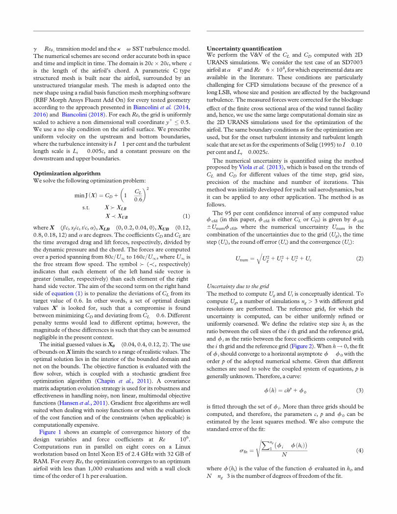
Uncertainty due to the gridThe method to compute Ug and Ut is conceptually identical. Tocompute Ug, a number of simulations ng > 3 with different gridresolutions are performed. The reference grid, for which theuncertainty is computed, can be either uniformly refined oruniformly coarsened. We define the relative step size hi as theratio between the cell sizes of the i th grid and the reference grid,and f i as the ratio between the force coefficients computed withthe i th grid and the reference grid (Figure 2).When h! 0, the fitof f i should converge to a horizontal asymptote f f 0 with theorder p of the adopted numerical scheme. Given that differentschemes are used to solve the coupled system of equations, p isgenerally unknown.Therefore, a curve:

f hð Þ ¼ chp 1 f 0 (3)

is fitted through the set of f i. More than three grids should becomputed, and therefore, the parameters c, p and f 0 can beestimated by the least squares method. We also compute thestandard error of the fit:

s fit ¼Xng

1f i f hið Þ� �N

s(4)

where f (hi) is the value of the function f evaluated in hi, andN ng 3 is the number of degrees of freedom of the fit.

g Reu t transition model and the k v SST turbulence model. The numerical schemes are second order accurate both in space and time and implicit in time. The domain is 20c � 20c, where c is the length of the airfoil’s chord. A parametric C type structured mesh is built near the airfoil, surrounded by an unstructured triangular mesh. The mesh is adapted onto the new shape using a radial basis function mesh morphing software (RBF Morph Ansys Fluent Add On) for every tested geometry according to the approach presented in Biancolini et al. (2014, 2016) and Biancolini (2018). For each Re, the grid is uniformly scaled to achieve a non dimensional wall coordinate y1 � 0.5. We use a no slip condition on the airfoil surface. We prescribe uniform velocity on the upstream and bottom boundaries, where the turbulence intensity is I 1 per cent and the turbulent length scale is Lt 0.005c, and a constant pressure on the downstream and upper boundaries.

Optimization algorithmWe solve the following optimization problem:

Uncertainty quantificationWe perform the V&V of the CL and CD computed with 2D URANS simulations. We consider the test case of an SD7003 airfoil at a 4° andRe 6� 104, for which experimental data are available in the literature. These conditions are particularly challenging for CFD simulations because of the presence of a long LSB, whose size and position are affected by the background turbulence. The measured forces were corrected for the blockage effect of the finite cross sectional area of the wind tunnel facility and, hence, we use the same large computational domain size as the 2D URANS simulations used for the optimization of the airfoil. The same boundary conditions as for the optimization are used, but for the onset turbulent intensity and turbulent length scale that are set as for the experiments of Selig (1995) to I 0.10 per cent and Lt 0.0025c.

The numerical uncertainty is quantified using the method proposed by Viola et al. (2013), which is based on the trends of CL and CD for different values of the time step, grid size, precision of the machine and number of iterations. This method was initially developed for yacht sail aerodynamics, but it can be applied to any other application. The method is as follows.

The 95 per cent confidence interval of any computed value f cfd (in this paper, f cfd is either CL or CD) is given by f cfd

6Unumf cfd, where the numerical uncertainty Unum is the combination of the uncertainties due to the grid (Ug), the time step (Ut), the round off error (Ur) and the convergence (Uc):

The extrapolated value f 0 is the expected value of f for aninfinitely fine grid. This allows estimating the error of thereference grid (Figure 2) as:

d ¼ j1 f 0j (5)

The grid uncertainty is then given by:

Ug ¼ 1:25 d 1s fit (6)

where 1.25 is a safety factor taken from the work of Roache(1998).Themain limitations of the proposedmethod are that we apply

the least squares method when the standard deviation of the erroris not constant, but it increases with h. This could be overcome,for instance, by doing the logarithmic of equation (3) and thenusing a linear fit instead of a non linear fit. However, given thanf 0 is unknown, its value should be optimized minimizing theresiduals of the fit, making the V&V unnecessarilyovercomplicated.Table I shows the number of cells and the maximum y1 of

the first cell centre for each grid, while Figure 3(a) shows thereference grid (Grid 4) in the near wall region. This grid has thesame chordwise and wall normal resolution as the 2D URANSsimulations of the optimal airfoils.

Other sources of uncertaintyA virtually identical procedure is used to computeUt, where sixdifferent time steps substitute the different grids used for the

computation of Ug. The reference time step is Dt 0.05c/U1,where a range ofDt from 0.0025c=U1 to 2.48c=U1 is explored.The uncertainty due to the convergenceUc is the 95 per cent

confidence interval in the estimate of the mean force coefficientin the time interval from 80c=U1 to 160c=U1:

Uc ¼ 1:646s

Nitp (7)

where s is the standard deviation of the Nit 1,600observations within this time interval.The round off error is estimated by running the simulations

in both single and double precision. Denoted with f r, the ratiobetween the force coefficients computed in single and doubleprecision, we estimate the error as:

d r ¼ j1 f rj (8)

and we compute the uncertainty as:

Ur ¼ 3 d r (9)

where 3 is a safety factor.As discussed in the Results section, the grid uncertainty of

the SD7003 airfoil is one order of magnitude larger than theother uncertainties. Therefore, for the optimum 4 digit NACAairfoils at Re 104, 105 and 106, we consider only the griduncertainty. For each Re, the grid is uniformly refined twice byhalving every cell.

Modelling errorValidationThe validation against experimental data allows an estimate ofthe modelling error of f cfd. This is given by the differencebetween the total error E and the validation uncertainty Uval,which are defined as:

E ¼ f cfd f exp (10)

and

Uval ¼ U2num 1U2

exp

q(11)

where f exp is the experimental estimate and Uexp is theexperimental uncertainty. If |E| > Uval, then the numericalerror has the sign of E. Conversely, if |E|� Uval, then f cfd is

Figure 1 Example of convergence history for Re = 106 of (a) the design variables and (b) the force coefficients

Figure 2 Schematic diagram of the method to compute the grid andtime step uncertainties

validated at the level ofUval and the modelling error is relativelytoo small to be assessed.

Comparison with other modelsTo gain more insight into the modelling error, we compare theaerodynamic forces, the surface pressures and the velocity fieldcomputed with different models: Xfoil, 2D URANS, 3DURANS and LES. Unfortunately, the experimental results ofSelig (1995) do not include information on the flow field;therefore, we compare with the measurements of Ol et al.(2005), which instead do not include force measurements. Wealso consider a slightly higher turbulence intensity, I 0.28 percent, to compare our results with those of Zhang et al. (2008).Xfoil is an inviscid linear vorticity panel code coupled with a

two equation lagged dissipation integral method (Drela, 1989).Transition is computed with the eN method. Following theexperimental correlations proposed by Mack (1977) and Ingen(2008), we set the Ncrit value to 5.7 corresponding to the freestream turbulence intensity of the wind tunnel (Zhang et al.,2008). The grid resolution and solver setting are kept asconsistent as possible between the different Navier Stokesmodels, so that the differences between 2D URANS and 3DURANS can largely be attributed to the additional dimension,and the differences between 3D URANS and LES can beattributed to the turbulencemodel.The domain size and the turbulent intensity used for this

comparison are different from those used for the V&V becauseof the different experimental conditions. The experiments ofSelig (1995) included an accurate measure of the aerodynamicforces and, therefore, are used for the V&V, whereas Zhanget al. (2008) performed flow measurements with particle imagevelocimetry (PIV), and thus, we use these tests for the analysisof the modelling error. PIV measurements cannot be correctedfor the blockage effect, and hence, the computational domainmatches the test section of this latter experiment, that is 6.25clong, 1.65c wide and 1.25c high. As this study of the modellingerror focuses on the flow field near the foil and not on theaerodynamic forces, which were not measured during theexperiment, we used a relatively short domain in the spanwisedirection. This could lead to overestimating the drag. Hence,

future work might include a sensitivity study of the effect of thestreamwise computational domain size.We set a no slip condition on the airfoil surface, a Dirichlet

type velocity condition on the upstream boundary, a symmetrycondition on the top and bottom boundaries and a Neumanntype pressure condition on the outlet boundary. For the 3DURANS and LES simulations, we set a symmetry condition onthe side boundaries. If we used a no slip condition for the sidewalls of the computational domain, we would have to resolvethe boundary layer on the walls of the facility. Conversely, theuse of the symmetry condition allows focusing the gridresolution in the region near the airfoil.To achieve a grid that is consistent between the three models

Dirichlet type 2D URANS, 3D URANS and LES Dirichlettype we build a new multi block structured grid [Figure 3(b)],where the resolution near the airfoil is the same as the referencegrid [Figure 3(a)]. This new grid used for the 2DURANSmodelis extruded spanwise by one third of the airfoil chord to make a3D grid that is equally suitable for the 3D URANS and LESmodels. In general, grid requirements for URANS and LES arevery different. In particular, the grid spacing in both thestreamwise and spanwise directions must be lower for LES thanURANS. In the present case, however, a high streamwise gridresolution is used across the whole foil for the 2D URANSsimulations to accurately resolve separation and reattachment,which occurs at different positions along the chord at every Re.Further, the grid used for the 3D URANS simulations is madewith high spanwise resolution,making it also suitable for the LESsimulation. The 2D grid has 6.4� 103 cells, whereas the 3D gridhas 6� 106 cells. The thickness of the near wall cells in the wallnormal direction is Dy 4 � 10– 4c, which allows y1 < 1. Thestreamwise cell aspect ratio is Dx/Dy 2 and the spanwise cellaspect ratio is Dz=Dy 7. A grid study was not performed for the3DRANSandLES, and it should be considered for future work.For the LES, we use a dynamic Smagorinsky Lilly model for

the sub grid stresses, a bounded central differencing scheme forthe spatial derivatives, a second order implicit scheme for theunsteady term in the momentum equation and a SIMPLEalgorithm for time marching with Dt 0.0025c=U1. A spectralsynthesizer method (Smirnov et al., 2001) is used to achieve

Table I Tested grids of the SD7003 airfoil at Re = 6� 104, a = 4°, I = 0.10 per cent

Grid 1 Grid 2 Grid 3 Grid 4 (ref) Grid 5 Grid 6

Number of cells 3.3� 103 6.4� 103 4.3� 104 5.4� 104 1.3� 105 4.7� 105

Maximum y1 2 1 0.5 0.1 0.1 0.05

Figure 3 Reference grids around the SD7003 airfoil used for the estimation of (a) the numerical uncertainty of the 2D URANS simulations and (b) themodelling error by comparison of the 2D URANS, 3D URANS and LES models

CL CD

Experiments (Selig, 1995) 0.570 0.0172D URANS 0.584 0.0208Ug 0.8% 0.1%Ut <10–5 <10–5

Ur <10–5 <10–5

Uc <10–5 <10–5

Unum 0.8% 0.1%|E| 2.5% 22%Uexp 1.5% NAUval 1.7% NAValidated at a level of Uval ? No NA

Re 104 105 106

Number of cells 23,000 34,000 64,000Max (y1) 0.4 0.07 0.01CL 0.57 0.64 0.60CD 0.0397 0.0141 0.00425Ug of CL (%) 8.4 3.1 0.003Ug of CD (%) 19.3 6.2 2.1

onset turbulence with I 0.285 per cent and Lt 0.0075c. The turbulence intensity decays from the inlet to the airfoil location, where I 0.280 per cent as reported in the experiments.

Results

The results are organized as follows. First, we discuss our estimate of the numerical and modelling errors. Successively we present the results of the optimization for different Re. Finally, we discuss the trends of the maximum efficiency and optimum thickness across with Re.

Uncertainty quantificationTable II summarizes the results of the V&V of the 2D URANS computations. The numerical uncertainty of CL is Unum 0.8 per cent, whereas the experimental uncertainty is Uexp 1.5 per cent (Selig, 1995), which results in a validation uncertainty of Uval 1.7 per cent. The absolute value of the error on the CL, |E| 2.5 per cent, is higher than Uval, and thus, CL is not validated at the level of 1.7 per cent. The simulation over estimates CL, but the error is not much higher than the validation uncertainty, leading to a low confidence in the sign of the modelling error. This error is further investigated in the next section.The numerical uncertainty of CD is 0.1 per cent.

Unfortunately, Selig (1995) did not provide a value for the experimental uncertainty, and thus, CD could not be validated. The absolute error of CD is similar to the one of CL, which is about 0.5 per cent of the dynamic pressure. However, given the smaller absolute value of CD compared with CL, the relative error of CD is significant. For the present application, an error of 22 per cent is sufficiently small compared with the differences in CD of ca. 300 per cent for every tenfold increase in Re (cf. Table III).For both CL and CD, the grid uncertainty is one order of

magnitude higher than the other uncertainties, and thus, Unum � Ug. We assume that the other sources of numerical uncertainties are negligible also for the 4 digit NACA airfoils. Therefore, we compute only Ug for the optimal airfoils. We consider Re 104, 105 and 106. Table III shows the number of cells, the maximum y1 and grid uncertainties for the reference grid at each Re. As for the SD7003 airfoil at Re 6 � 104, the grid uncertainties are higher for CD than for

Table II V&V on the SD7003 airfoil at Re = 6 � 104, a = 4°, I = 0.10 per cent

CL. Ug decreases with Re both for CL and CD. The uncertainties computed for the SD7003 airfoil at Re 6 � 104

are similar to those computed for the optimum 4 digit NACA foil at Re 105. The maximum uncertainty is Ug of CD (19.3 per cent) for the lowest tested Re (104). Recalling that CD decreases by about 300 per cent for a tenfold increase in Re, the maximum value of Ug of CD is sufficiently small to compute the trend of CD across the proposed range of Re.

Modelling errorTo investigate the source of the modelling error, we compare the flow fields computed with our simulations and the experimental and numerical results of other authors. Table IV shows CL, CD and the chordwise coordinates of the separation point (xs), of the transition point (xt) and of the reattachment point (xr). The transition point is defined as the locum where hu0v0i=U2 ¼ 10�3, where u0 and v0 are the velocity fluctuations in the dra

1g and lift directions, respectively.

Between this set of results, all numerical simulations overpredict CL and CD by a similar amount. The minimum CL

is computed by our 2D URANS simulations, whereas only Xfoil predicts a slightly lower CD than 2D URANS. All numerical simulations predict an earlier separation point than the experiments, and a similar transition and reattachment point. This analysis suggests that the modelling error is not due to the 3D effect or to the turbulence model.We further investigate the modelling error considering a

different set of experiments (Zhang et al., 2008), where the turbulence intensity is I 0.28 per cent instead of I 0.10 per cent. We model these experiments with Xfoil, 2D URANS, 3D URANS and LES. Table V shows a summary of the results. All models overpredict CL by more than the 2D URANS simulations, and only Xfoil predicts a closer CD to the experimental value. With the higher turbulence intensity, xs=c is well predicted by all models. Both URANS simulations made a similar prediction.For both values of turbulence intensity, the transition

point xt=c is better predicted by LES. The region of turbulent flow near the airfoil is shown by the contour of hu0v0i=U2 in Figure 4, which also includes the experimental

1results (Zhang

et al., 2008). LES also predicts a higher growth rate of turbulent fluctuations than the other models, resulting in an earlier reattachment and a thinner turbulent boundary layer (cf. also Figure 5).Figure 5 shows the shape of the LSB and the growth of the

reattached boundary layer through streamlines and contours of non dimensional flow speed juj/U1, where juj is the magnitude of the velocity vector. The shorter LSB and the thinner reattached boundary layer of the LES solution result in a higher

Table III Reference grids and Ug for the optimum 4-digit NACA airfoils

L and lower D. Figure 6a shows the pressure coefficient Cp

along the chord of the airfoil. LES and 2D URANS predictedthe lowest and the highest pressure plateau, which is correlatedwith the LSB, and themaximum andminimum L, respectively.The reattachment is correlated with the point of maximumpressure gradient downstream of the plateau. Figure 6(b)shows large differences between the streamwise Cf valuescomputed by the different models. The reattached thinner andmore energetic boundary layer predicted by LES is correlatedwith a significantly increased Cf. However, this does not resultin a higherD because the friction drag is more than one order ofmagnitude smaller than the pressure drag.In conclusion, a comparison of the experimental flow

measurements and the LES, 3D URANS and 2D URANSsolutions shows that although LES provides the most accuratesolution, the bidimensionality of the 2D URANS simulationsdoes not lead to a significant increase in the modelling errorwhen compared with 3D URANS. Importantly, the 2DURANS simulations are capable of correctly predicting thegeneral features of the LSB.

Optimum airfoil shapesAs the above results have grown our confidence in thenumerical results achieved with 2D URANS simulations, wenow consider the optimum airfoil geometry computed fordifferent Re. For each Re from 104 to 3 � 106, Figure 7shows the optimum geometry and the correlated velocityfield juj/U1. At the lowest value of Re investigated, Re 104,the boundary layer is laminar and the optimum airfoilpresents a very small curvature for most of the chord to delayseparation, which occurs on the upper side at xs=c 0.81.Downstream of the separation point, the curvature increasesto generate lift. At Re 3 � 104, laminar separation does notoccur; therefore, a higher curvature may be exploited in thefirst half of the chord for lift generation. The flatter trailingedge then prevents separation over the second half of thechord. At Re 105, we find a long LSB. Near the leadingedge, a high curvature provides lift but in this case promotesseparation (xs=c 0.25), whereas downstream of theseparation point, the airfoil has almost no curvature topromote turbulent reattachment (xr=c 0.65) and theformation of a long LSB. At Re 3 � 105, a more uniformcurvature allows the separation point to be furtherdownstream (xs=c 0.61); transition occurs closer to theseparation point, leading to a shorter LSB (xr=c 0.75) andan advantageous thinner wake. At Re 106, transitionoccurs in the attached boundary layer; the turbulentboundary layer remains attached along the entire airfoil. Analmost constant curvature on the upper side leads to a verythin wake and low drag. Finally, at the highest Re evaluated,Re 3 � 106, the increased resilience of the turbulentboundary layer to separation allows the area of highestcurvature, and thus highest adverse pressure gradient, to be

Table IV Comparison with other authors for the SD7003 airfoil at Re = 6� 104, a = 4°, I = 0.10 per cent

Model Reference I CL CD xs=c xt=c xr=c

Exp Selig (1995) 0.10 0.570 0.017 NA NA NAExp Ol et al. (2005) 0.10 NA NA 0.30 0.53 0.62Xfoil Present results 0.10 0.618 0.019 0.22 0.54 0.572D URANS Radespiel et al. (2007) 0.08 0.60 0.020 NA 0.57 0.622D URANS Present results 0.10 0.584 0.0208 0.20 0.50 0.70LES Catalano and Tognaccini (2010) 0.10 0.63 0.0225 0.21 0.53 0.65

Table V Summary of results for the SD7003 airfoil at Re = 6 � 104,a = 4°, I = 0.28 per cent

Model Reference I CL CD xs=c xt=c xr=c

Exp Zhang et al. (2008) 0.28 NA NA 0.21 0.40 0.51Xfoil Present results 0.28 0.605 0.018 0.24 0.48 0.522D URANS Present results 0.28 0.586 0.0222 0.18 0.46 0.643D URANS Present results 0.28 0.669 0.0237 0.21 0.45 0.63LES Present results 0.28 0.670 0.0219 0.22 0.42 0.57

Figure 4 Contours of Reynolds stresses around the SD7003 airfoil tested at Re = 6� 104, a = 4°, I = 0.28 per cent

moved furthest toward the trailing edge. This again has theadditional advantage of minimizing wake thickness and thusdrag.

Maximum efficiencyThe wake’s thickness, which is correlated with the drag,decreases monotonically with Re despite the complexrelationship between the flow field, the airfoil geometry and theReynolds number. Noting that CL 0.6 at every Re, thedecrease in wake thickness results in an increase of L/DwithRe.In Figure 8, we compare our results (black filled dots) achieved

optimizing the airfoil shape for every Re, with those of otherauthors who tested individual airfoils across a range of Re. Forexample, McMaster and Henderson (1980) identified aninterval of Re between 104 and 106 (region between solid linesmarked with dots), where the L/D of most smooth airfoilsincreases from less than 10 to more than 100. Conversely,rough foils have a more gentle increase of L/D versus Re (regionbetween short dash lines marked with waves), due to theirability to promote transition near the leading edge. Similarly,Schmitz (1967) found that flat plates have a smoother L/Dtrend (long dash line) because leading edge separationpromotes transition.

Figure 5 Contours of velocity and streamlines around the SD7003 airfoil at Re = 6� 104, a = 4°, I = 0.28 per cent

Figure 6 (a) Pressure coefficient and (b) streamwise friction coefficient for the SD7003 airfoil tested at Re = 6� 104, a = 4°, I = 0.28 per cent

Figure 7 Contours of flow speed around the optimum airfoils for different Re

At the lowest Re tested, Re 104, the 4 digit NACA airfoilsperform better than flat plates. However, the visualextrapolation of our results toward lower Re suggests that, atRe 103, a 4 digit NACA airfoil would have similarperformance than a flat plate. Our optimal airfoils have higherL/D than those presented byMcMaster and Henderson (1980)at Re 104 and 3 � 104 and similar L/D at Re 105 and 106.This is not surprising given that the foils that McMaster andHenderson tested were optimized for critical and supercriticalRe. Only specialized airfoils that adopt a “laminar rooftop”,such as those developed by Liebeck (1978), allow much higherefficiency at highRe.

Optimum thicknessIt has been observed that thinner airfoils allow higher efficiencythan thicker airfoils at low Re. Lilienthal (1911), who studiedbird wings at low Re, noted for the first time that curved thinplates performed better than thick airfoils. When the influenceof Re was then better understood, it was found that airfoilefficiency increases with Re, and eventually exceeds that of thinplates (Schmitz, 1967). Sunada et al. (1997, 2002) tested arange of airfoils and flat and curved plates at Re 4 � 103 andfound that, at such low Re, the curved plates are the most

efficient. Lissaman (1983) compared wing sections of efficientfliers at increasing Re: from insects, through birds, to aircrafts,and noted that the thickness to chord ratio of these sectionsincreased with Re. Figure 8 shows the efficiency of thedragonfly Anisoptera, the pigeon Columbidae, the SD7003 andthe NACA4412, which all fit the trend suggested byMcMasters andHenderson (1980) for smooth airfoils.The proposed monotonic increase of t/c with Re is not

confirmed by present results. In fact, as shown in Figure 9(a),t/c is roughly a step function of Re, with the step occurringbetween Re 105 and 3 � 105; the point from which withincreasing Re, the boundary layer remains attached along theentire airfoil. The trend of xf=c with Re is also non monotonic:xf=c decreases when trailing edge separation occurs, and thenincreases for higher Re [Figure 9(b)]. Conversely, f=c � 3 percent for every Re. Therefore, we conclude that to generate aconstant CL 0.6, the optimal camber remains constant,whereas the angle of attack is varied to achieve the desired lift.

Conclusions

In this paper, we propose a numerical model for theoptimization of airfoils across a range of Reynolds numbers(Re) from 104 to 3 � 106. We consider 2D unsteady

Figure 8 Airfoil efficiency for a range of Reynolds numbers from the literature and present results

Figure 9 Trends of the design variables with Re

pp. 823 877, doi: 10.1177/1045389X11414084.Barlas, T.K. and van Kuik, G.A.M. (2010), “Review of state ofthe art in smart rotor control research for wind turbines”,Progress in Aerospace Sciences, Vol. 46, pp 1 27, doi: 10.1016/j.paerosci.2009.08.002.

Biancolini, M.E. (2018), Fast Radial Basis Functions forEngineering Applications, Springer International Publishing,doi: 10.1007/978 3 319 75011 8.

Biancolini, M.E., Viola, I.M. and Riotte, M. (2014), “Sailstrim optimisation using CFD and RBF mesh morphing”,Computers & Fluids, Vol. 93, pp. 46 60, doi: 10.1016/j.compfluid.2014.01.007.

Biancolini, M.E., Costa, E., Cella, U., Groth, C., Veble, G.and Andrejašic, M. (2016), “Glider fuselage wing junctionoptimization using CFD and RBF mesh morphing”,Aircraft Engineering and Aerospace Technology, Vol. 88 No. 6,pp. 740 752, doi: 10.1108/aeat 12 2014 0211.

Bot, P., Rabaud, M., Thomas, G., Lombardi, A. and Lebret,C. (2016), “Sharp transition in the lift force of a fluid flowingpast nonsymmetrical obstacles: evidence for a lift crisis in thedrag crisis regime”, Physical Review Letters, Vol. 117 No. 23,p. 234501, doi: 10.1103/PhysRevLett.117.234501.

Carmichael, B.H. (1981), “Low Reynolds number airfoilsurvey”,NASATechnical Report CR 165803, Vol. 1.

Catalano, P. and Tognaccini, R. (2010), “Numerical analysisof the flow around the SD 7003 airfoil”, 48th AIAAAerospaceSciences Meeting Including the New Horizons Forum andAerospace Exposition, 4 7 January 2010, Orlando, Florida,available at: https://doi.org/10.2514/6.2010 68

Celik, I. (2003), “RANS/LES/DES/DNS: the future prospectsof turbulence modeling”, Journal of Fluids Engineering,Vol. 127No. 5, pp. 829 830, doi: 10.1115/1.2033011.

Chapin, V., De Carlan, N. and Heppel, P. (2011),“Performance optimization of interacting sails through fluidstructure coupling”, In: International Journal of Small CraftTechnology 153. Part B2, pp. 103 116, available at: http://oatao.univ toulouse.fr/5262/

Crabtree, L.F. (1959), The Formation of Regions of SeparatedFlow onWing Surfaces, HMStationeryOffice.

Drela, M. (1989), “XFOIL: an analysis and design system forlow Reynolds number airfoils”, Low Reynolds NumberAerodynamics, Springer, pp. 1 12.

Drela, M. (1998), “Pros and cons of airfoil optimization”,Proceedings of Frontiers of Computational Fluid Dynamics,pp. 363 381, available at: https://doi.org/10.1142/3975

Hansen, M.O.L., Sørensen, J.N., Voutsinas, S., Sørensen, N.and Madsen, H.A. (2006), “State of the art in wind turbineaerodynamics and aeroelasticity”, Progress in AerospaceSciences, Vol. 42 No. 4, pp. 285 330, doi: 10.1016/j.paerosci.2006.10.002.arXiv:arXiv:1006.4405v1.

Hansen, N., Ros, R., Mauny, N., Schoenauer, M. and Auger,A. (2011), “Impacts of invariance in search: when CMA ESand PSO face ill conditioned and non separable problems”,Applied Soft Computing, Vol. 11 No. 8, pp. 5755 5769, doi:10.1016/j.asoc.2011.03.001.

Hicks, R.M. and Henne, P.A. (1978), “Wing design bynumerical optimization”, Journal of Aircraft, Vol. 15 No. 7,pp. 407 412, doi: 10.2514/3.58379.

Hu, H. and Tamai, M. (2008), “Bioinspired corrugated airfoilat low Reynolds numbers”, Journal of Aircraft, Vol. 45 No. 6,pp. 2068 2077, doi: 10.2514/1.37173.

Ingen, J.L.V. (2008), “The eN method for transitionprediction. Historical review of work at TU Delft”, 38thAIAA Fluid Dynamics Conference and Exhibit, AIAA paper2008 3830, Seattle,Washington, 23 26 June 2008, pp. 1 49.

incompressible flow, a g Reu t transition model with a k v SST turbulence model, and we couple the fluid solver with a covariance matrix adaptation evolutionary optimization algorithm. We use this approach to find the optimal 4 digit NACA airfoil that maximizes the lift over drag ratio allowing an arbitrary chosen lift coefficient of 0.6.We investigate the numerical and modelling errors

performing 3D simulations with the same numerical setup, large eddy simulations and Xfoil simulations, in addition to comparisons with experimental data available in the literature. We show that the 2D simulations allow the prediction of the separation, transition and reattachment within approximately 10 per cent of the chord compared with experimental data. In the range of validity of Xfoil, i.e. when natural laminar to turbulent transition occurs and separation is limited within an LSB, it shows comparable performances. The 3D simulations do not offer a significant improvement compared with the 2D simulations, whereas the large eddy simulations allow a better prediction of the transition and reattachment locations.At transitional Reynolds numbers, the largest numerical

uncertainty is the one due to the grid resolution and it decreases with Re. For the lift coefficient, it ranges from 8 per cent to 0.003 per cent, and for the drag coefficient, it ranges from 19 per cent to 2 per cent. We find approximately the same grid uncertainties also for a similar test case of an SD7003 airfoil at Re 6 � 104, where experimental data are available. For this case, the uncertainties due to the time resolution, the round off error and the convergence are all more than one order of magnitude smaller. These levels of uncertainty are sufficiently small to evaluate the performances of an airfoil across the range of Re considered. In fact, the lift over drag ratio of the optimal 4 digit NACA airfoils increases by 300 per cent for every tenfold increase in Re.It has been observed that the thickness to chord ratio of

wing sections of efficient fliers, both man made and natural, increases monotonically with Re. Our results, however, show that the optimal thickness does not increase monotonically. On the contrary, it is almost constant at low and high Re and shows a step increase when Re is sufficiently high to prevent separation or to allow reattachment and the formation of an LSB. To generate a constant lift coefficient, which is largely dictated by angle of attack and camber, the angle of attack decreases monotonically with Re, whereas the camber remains ca. 3 per cent at every Re. These results suggest that the airfoil shapes of insect and bird wings, that are the consequence of natural evolution, may not be aerodynamic optima when considering solely the maximization of lift to drag ratio.

References

Barbarino, S., Bilgen, O., Ajaj, R.M., Friswell, M.I. and Inman, D.J. (2011), “A review of morphing aircraft”, Journal of Intelligent Material Systems and Structures, Vol. 22 No. 9,

Klanfer, L. and Owen, P.R. (2018), The Effect of IsolatedRoughness on Boundary Layer Transition, R.A.E. Tech.Memo.No. Aero. 355.

Kuder, I.K., Arrieta, A.F., Raither, W.E. and Ermanni, P.(2013), “Variable stiffness material and structural conceptsfor morphing applications”, Progress in Aerospace Sciences,Vol. 63, pp. 33 55, doi: 10.1016/j.paerosci.2013.07.001.

Lachenal, X.S., Daynes, P.M. and Weaver, (2013), “Review ofmorphing concepts and materials for wind turbine bladeapplications”, Wind Energy, Vol. 16 No. 2, pp. 283 307, doi:10.1002/we.531.arXiv:arXiv:1006.4405v1.

Langtry, R. and Menter, F. (2005), “Transition modeling forgeneral CFD applications in aeronautics”, 43rd AIAAAerospace Sciences Meeting and Exhibit, AIAA 2005 522,doi: 10.2514/6.2005 522.

Liebeck, R.H. (1978), “Design of subsonic airfoils for highlift”, Journal of Aircraft, Vol. 15 No. 9, pp. 547 561, doi:10.2514/3.58406.

Lilienthal, O. (1911), Birdflight as the Basis of Aviation: AContribution towards a System of Aviation, Compiled from theResults of Numerous Experiments Made by O. and G. Lilienthal,Green, Longmans.

Lissaman, P.B.S. (1983), “Low Reynolds number airfoils”,Annual Review of Fluid Mechanics, Vol. 15, pp. 223 239, doi:10.1146/annurev.fl.15.010183.001255.

McMasters, J. and Henderson, M. (1980), “Low speedsingle element airfoil synthesis”, NASA Langley ResearchCenter, Science and Technology of Low Speed and MotorlessFlight, Part 1, pp. 1 31.

Mack, L.M. (1977), “Transition and laminar instability”, JetPropulsion Laboratory Pub, NASA Technical Reports Server,NASA CR 153203, JPL PUBL 77 15, pp. 77 115.

Menter, F.R., Langtry, R. and Völker, S. (2006), “Transitionmodelling for general purpose CFD codes”, Flow, Turbulenceand Combustion, Vol. 77Nos 1/4, pp. 277 303.

Minervino, M., Vitagliano, P.L. and Quagliarella, D. (2016),“Helicopter stabilizer optimization considering rotordownwash in forward flight”, Aircraft Engineering andAerospace Technology, Vol. 88 No. 6, pp. 846 865, doi:10.1108/AEAT 03 2015 0082.

Moin, P. and Mahesh, K. (1998), “Direct numericalsimulation: a tool in turbulence research”, Annual Review ofFluid Mechanics, Vol. 30, pp. 539 578, doi: 10.1146/annurev.fluid.30.1.539.

Ol, M., McCauliffe, B., Hanff, E., Scholz, U. and Kähler, C.(2005), “Comparison of laminar separation bubblemeasurements on a low Reynolds number airfoil in threefacilities”, in 35th AIAA Fluid Dynamics Conference andExhibit, 6 9 June,Toronto, Ontario, p. 5149.

Pasquale, D., Di, A., Rona, S.J. and Garrett (2009), “Aselective review of CFD transition models”, 39th AIAA FluidDynamics Conference, 22 25 June, AIAA 2009 3812, SanAntonio, Texas, doi: 10.2514/6.2009 3812.

Radespiel, R.E., Windte, J. and Scholz, U. (2007), “Numericaland experimental flow analysis of moving airfoils withlaminar separation bubbles”, AIAA Journal, Vol. 45 No. 6,pp. 1346 1356, available at: https://doi.org/10.2514/1.25913

Roache, P.J. (1998), “Verification of codes and calculations”,AIAA Journal, Vol. 36 No. 5, pp. 696 702, available at:https://doi.org/10.2514/2.457

Mathematical, Physical and Engineering Sciences, Vol. 367No. 1899, pp. 2849 2860, doi: 10.1098/rsta.2008.0269.

Schmitz, F.W. (1967), “Aerodynamics of the model airplane.Part 1 Airfoil measurements”, in Selig, M.S. (1995),Summary of Low Speed Airfoil Data. Summary of LowSpeed Airfoil Data v.1, SoarTech Publications, available at:https://books.google.it/books?id qtIeAQAAIAAJ

Schmitz, F.W. (2003), “Low Reynolds number airfoil designlecture notes various approaches to airfoil design”,VKILectureSeries November, pp. 24 28, available at: www.ae.illinois.edu/mselig/pubs/Selig 2003 VKI LRN Airfoil Design LectureSeries.pdf

Smirnov, A., Shi, S. and Celik, I. (2001), “Random flowgeneration technique for large eddy simulations and particledynamics modeling”, Journal of Fluids Engineering, Vol. 123No. 2, pp. 359, doi: 10.1115/1.1369598.

Smith, A.M.O. and Gamberoni, N. (1956), “Transition,pressure gradient, and stability theory”, Douglas AircraftCompany, El SegundoDivision, Report Number ES 26388.

Smith, A.M.O. (1975), “High lift aerodynamics”, Journal ofAircraft, Vol. 12No. 6, pp. 501 530, doi: 10.2514/3.59830.

Spalart, P.R. (2009), “Detached eddy simulation”, AnnualReview of Fluid Mechanics, Vol. 41, pp. 181 202, doi:10.1146/annurev.fluid.010908.165130.

Squires, K.D. (2004), “Detached eddy simulation: currentstatus and perspectives”,Direct and Large Eddy Simulation VProceedings, ERCOFTAC Series, Vol. 9, pp. 465 480,available at: https://doi.org/10.1007/978 1 4020 2313 2 49

Srinath, D.N. and Mittal, S. (2010), “Optimal aerodynamicdesign of airfoils in unsteady viscous flows”, Computer Methodsin Applied Mechanics and Engineering, Vol. 199, Nos 29/32, pp.1976 1991, doi: 10.1016/j.cma.2010.02.016

Stanewsky, E. (2001), “Adaptive wing and flow controltechnology”, Progress in Aerospace Sciences, Vol. 37 No. 7,pp. 583 667, doi: 10.1016/S0376 0421(01)00017 3.

Sunada, S., Sakaguchi, A. and Kawachi, K. (1997),“Airfoil section characteristics at a low Reynoldsnumber”, Journal of Fluids Engineering, Vol. 119 No. 1,pp. 129 135, doi: 10.1115/1.2819098.

Sunada, S., Yasuda, T., Yasuda, K. and Kawachi, K. (2002),“Comparison of wing characteristics at an ultralow Reynoldsnumber”, Journal of Aircraft, Vol. 39 No. 2, pp. 331 338,available at: https://doi.org/10.2514/2.2931

Tully, S. and Viola, I.M. (2016), “Reducing the wave inducedloading of tidal turbine blades through the use of a flexibleblade”, International Symposium on Transport Phenomena andDynamics of Rotating Machinery (ISROMAC 2016), 10 15April, Honolulu, Hawaii, p. 9, available at: https://hal.archives ouvertes.fr/hal 01517948/document

Viola, I.M., Bot, P. and Riotte, M. (2013), “On the uncertaintyof CFD in sail aerodynamics”, International Journal forNumerical Methods in Fluids, Vol. 72 No. 11, pp. 1146 1164,doi: 10.1002/fld.3780.arXiv:fld.1[DOI:10.1002].

Ward, J.W. (1963), “The behaviour and effects of laminarseparation bubbles on aerofoils in incompressible flow”, Journalof the Royal Aeronautical Society, Vol. 67 No. 636, pp. 783 790,available at: https://doi.org/10.1017/S0001924000061583

Sagaut, P. and Deck, S. (2009), “Large eddy simulation for aerodynamics: status and perspectives”, Philosophical Transactions of the Royal Society of London A:

Wu, X. and Moin, P. (2009), “Direct numerical simulation ofturbulence in a nominally zero pressure gradient flat plateboundary layer”, Journal of Fluid Mechanics, Vol. 630,pp. 5 41, doi: 10.1017/S0022112009006624.

Zhang, W., Hain, R. and Ahler, C.J.K. (2008), “Scanning PIVinvestigation of the laminar separation bubble on a SD7003

airfoil”, Experiments in Fluids, Vol. 45 No. 4, pp. 725 743,doi: 10.1007/s00348 008 0563 8.

Corresponding authorMarco Evangelos Biancolini can be contacted at:biancolini@ing.uniroma2.it

For instructions on how to order reprints of this article, please visit our website:www.emeraldgrouppublishing.com/licensing/reprints.htmOr contact us for further details: permissions@emeraldinsight.com