Optical system design for femtosecond-level synchronization of clocks Laura C. Sinclair1, William C. Swann1, Jean-Daniel Deschênes1,2, Hugo Bergeron1,2, Fabrizio R.

Giorgetta1, Esther Baumann1, Michael Cermak1, Ian Coddington1, and Nathan R. Newbury1

1National Institute for Standards and Technology, 325 Broadway, Boulder, CO 80305 2Université Laval, 2325 Rue de l’Université, Québec, QC, G1V 0A6, Canada

ABSTRACT

Synchronization of optical clocks via optical two-way time-frequency transfer across free-space links can result in time

offsets between the two clocks below tens of femtoseconds over many hours. The complex optical system necessary to

support such synchronization is described in detail here.

Work of the U.S. government, not subject to copyright.

Keywords: optical two-way time-frequency transfer, optical synchronization, optical metrology, frequency comb

1. INTRODUCTION

Recently, we have demonstrated the tight synchronization of two optical clocks to within femtoseconds across a 4 km

turbulent air path.1 To achieve this level of performance, we use optical two-way time-frequency transfer (O-TWTFT)

which removes the picosecond-level turbulence-induced timing fluctuations present on a one-way measurement to

achieve femtosecond-level synchronization. Here, we will discuss the optical system design which makes this

performance possible.

Figure 1. Overview of synchronization system. The coherent pulse train generated by the clock is combined with a coarse timing and

communications signal before being launched over the turbulent air path. The arrival of the coherent pulse train (clock signal) from

each site is detected with femtosecond precision at the other site. The coarse timing accounts for any ambiguities associated with the

separation between coherent pulses, while the communications signal allows for real time computation of the clock difference at the

remote site. Feedback is then applied to the remote clock to maintain synchronization between the two clocks, i.e. a time offset of

zero at a chosen reference plane.

Figure 1 shows a simplified schematic of the overall O-TWTFT system. Tight synchronization of two clocks to within

femtoseconds via O-TWTFT requires five basic steps:

1. The “ticks” of the optical clock must be generated with low pulse-to-pulse timing jitter, which requires an optical

oscillator (cavity stabilized laser) and associated phase-locked frequency comb.

2. The timing signal must be sent from one site to the other site and detected with femtosecond precision. As the

name suggests, for O-TWTFT, the transfer of clock signals must be bi-directional to cancel fluctuations due to

turbulence and platform motion.

3. The timing signals recorded at the master site must be communicated to the remote site. (Here, we refer to the

actively synchronized clock as the remote clock.)

4. Based on the two-way timing signals, the controller at the remote site must compute the time offset between the

two clocks in realtime.

Turbulent air path

Controller

Coarse timing

and ranging +

Communication

Coarse timing

and ranging +

Communication

Controller

Feedback

5. Feedback must be applied to the remote clock to drive the computed time offset between the two clocks to zero at

the chosen reference plane.

In O-TWTFT, two different sets of bi-directional timing signals are transmitted, one via frequency comb pulses and one

via an rf phase-modulated optical-carrier-wave. This optical carrier wave is also used to transmit the timing information

from the master site back to the remote site (step 3 above).

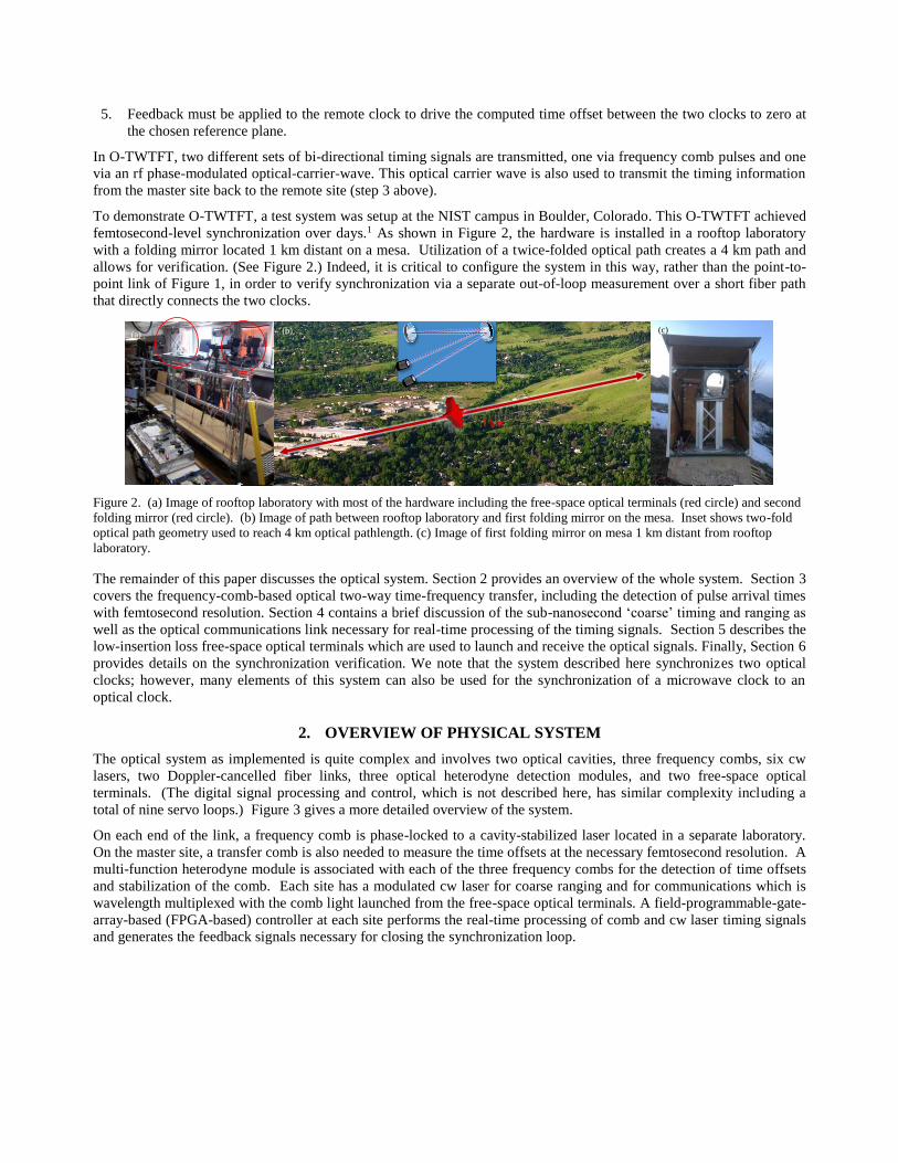
To demonstrate O-TWTFT, a test system was setup at the NIST campus in Boulder, Colorado. This O-TWTFT achieved

femtosecond-level synchronization over days.1 As shown in Figure 2, the hardware is installed in a rooftop laboratory

with a folding mirror located 1 km distant on a mesa. Utilization of a twice-folded optical path creates a 4 km path and

allows for verification. (See Figure 2.) Indeed, it is critical to configure the system in this way, rather than the point-to-

point link of Figure 1, in order to verify synchronization via a separate out-of-loop measurement over a short fiber path

that directly connects the two clocks.

Figure 2. (a) Image of rooftop laboratory with most of the hardware including the free-space optical terminals (red circle) and second

folding mirror (red circle). (b) Image of path between rooftop laboratory and first folding mirror on the mesa. Inset shows two-fold

optical path geometry used to reach 4 km optical pathlength. (c) Image of first folding mirror on mesa 1 km distant from rooftop

laboratory.

The remainder of this paper discusses the optical system. Section 2 provides an overview of the whole system. Section 3

covers the frequency-comb-based optical two-way time-frequency transfer, including the detection of pulse arrival times

with femtosecond resolution. Section 4 contains a brief discussion of the sub-nanosecond ‘coarse’ timing and ranging as

well as the optical communications link necessary for real-time processing of the timing signals. Section 5 describes the

low-insertion loss free-space optical terminals which are used to launch and receive the optical signals. Finally, Section 6

provides details on the synchronization verification. We note that the system described here synchronizes two optical

clocks; however, many elements of this system can also be used for the synchronization of a microwave clock to an

optical clock.

2. OVERVIEW OF PHYSICAL SYSTEM

The optical system as implemented is quite complex and involves two optical cavities, three frequency combs, six cw

lasers, two Doppler-cancelled fiber links, three optical heterodyne detection modules, and two free-space optical

terminals. (The digital signal processing and control, which is not described here, has similar complexity including a

total of nine servo loops.) Figure 3 gives a more detailed overview of the system.

On each end of the link, a frequency comb is phase-locked to a cavity-stabilized laser located in a separate laboratory.

On the master site, a transfer comb is also needed to measure the time offsets at the necessary femtosecond resolution. A

multi-function heterodyne module is associated with each of the three frequency combs for the detection of time offsets

and stabilization of the comb. Each site has a modulated cw laser for coarse ranging and for communications which is

wavelength multiplexed with the comb light launched from the free-space optical terminals. A field-programmable-gate-

array-based (FPGA-based) controller at each site performs the real-time processing of comb and cw laser timing signals

and generates the feedback signals necessary for closing the synchronization loop.

(a) (b) (c)

1 km

Figure 3. Schematic of synchronization system highlighting the physical system. On the master site, a second transfer comb is

implemented for detection of time offsets at the femtosecond level as discussed in Section 2.2 and Section 3.1. The optical cavities

and cavity-stabilized lasers are located in a separate laboratory and connected via Doppler-cancelled fiber links. The multi-function

heterodyne modules contain elements for launching comb light across the link, detecting the incoming timing signals, and phase-

locking the frequency combs to the cavity-stabilized lasers. The optical path is folded to allow for synchronization verification. (One

potential source of confusion is that sub-systems within a clock site are often tightly coupled physically to avoid systematic timing

drifts even if they might be separated in a conceptual diagram. For instance the heterodyne module both detects the optical signal to

phase-lock the frequency comb to the cavity stabilized laser and detects the timing signals from the incoming optical pulse train.)

Before discussing the design of the optical subsystems in more detail, we discuss two important underlying operations:

the generation of the optical timescale at each site and the calculation of the overall master synchronization equation.

2.1 Generating a Clock Output

At both the master and remote site, we must construct a clock. Here, we do so by tightly phase-locking a frequency

comb to a cavity-stabilized laser. The frequency comb at each site coherently converts the ~100 THz optical frequency

of the cavity-stabilized laser to the more accessible “clock tick” comb repetition frequency of ~200 MHz. (See Figure

4.) The time output of the clock then consists of the labeled pulse train generated by the frequency comb with the time

defined by the arrival of a pulse at a chosen reference plane. When operating synchronously, the repetition frequency for

the master and remote combs are identical and the two pulse trains overlap at a common reference plane. Note that for

continuous time output, as opposed to the more standard frequency output, the combs cannot exhibit any phase-slips.

Roof-top laboratory

Lower laboratory

Transfer Comb HeterodyneModule

HeterodyneModule

fr

Remote Comb

cavity-stabilizedlasers

fr + D fr

Master Comb

HeterodyneModule

Feedback

Optical Communication /Coarse (<ns) timing

Optical Communication /Coarse (<ns) timing

Transfer Remote D

Remote Transfer D

Transfer Master D

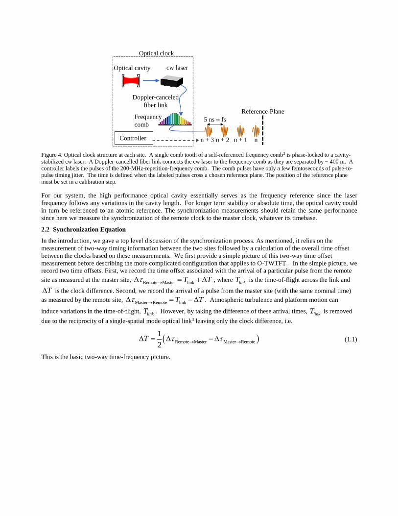
Figure 4. Optical clock structure at each site. A single comb tooth of a self-referenced frequency comb2 is phase-locked to a cavity-

stabilized cw laser. A Doppler-cancelled fiber link connects the cw laser to the frequency comb as they are separated by ~ 400 m. A

controller labels the pulses of the 200-MHz-repetition-frequency comb. The comb pulses have only a few femtoseconds of pulse-to-

pulse timing jitter. The time is defined when the labeled pulses cross a chosen reference plane. The position of the reference plane

must be set in a calibration step.

For our system, the high performance optical cavity essentially serves as the frequency reference since the laser

frequency follows any variations in the cavity length. For longer term stability or absolute time, the optical cavity could

in turn be referenced to an atomic reference. The synchronization measurements should retain the same performance

since here we measure the synchronization of the remote clock to the master clock, whatever its timebase.

2.2 Synchronization Equation

In the introduction, we gave a top level discussion of the synchronization process. As mentioned, it relies on the

measurement of two-way timing information between the two sites followed by a calculation of the overall time offset

between the clocks based on these measurements. We first provide a simple picture of this two-way time offset

measurement before describing the more complicated configuration that applies to O-TWTFT. In the simple picture, we

record two time offsets. First, we record the time offset associated with the arrival of a particular pulse from the remote

site as measured at the master site, Remote Master linkT T D D , where

linkT is the time-of-flight across the link and

TD is the clock difference. Second, we record the arrival of a pulse from the master site (with the same nominal time)

as measured by the remote site, Master Remote linkT T D D . Atmospheric turbulence and platform motion can

induce variations in the time-of-flight, linkT . However, by taking the difference of these arrival times,

linkT is removed

due to the reciprocity of a single-spatial mode optical link3 leaving only the clock difference, i.e.

Remote Master Master Remote

1

2T D D D (1.1)

This is the basic two-way time-frequency picture.

Frequency

comb

cw laserOptical cavity

Reference Plane

Doppler-canceled

fiber link

5 ns fs

Optical clock

Controller nn + 1n + 2n + 3

However, direction detection of the comb pulses with femtosecond resolution is not possible and as a consequence we

implement the transfer comb as discussed in Section 3.1. Now, three time offsets must be recorded: the arrival of the

transfer comb pulses as measured at the remote site, Transfer Remote D , the arrival of the remote comb pulses as

measured at the master site (by the transfer comb as described later), Remote Transfer D , and the time offset between the

transfer and master comb pulses, Transfer Master D . (See Figure 3.) There are ambiguities associated with each of these

time offset measurement because the comb pulses are separated by only 1/fr~ 5 nsec; these must be removed by a

“coarser” two-way time-frequency measurement. As given in Ref. 1, we have developed a master synchronization

equation that combines all these measurements to calculate the time offset between the master and remote clocks, TD .

This equation is:

r

Remote Transfer Transfer Remote Master Transfer cal link ADC

r r

1

2 2 2

f nT T t

f f

D DD D D D D

(1.2)

where rf is the repetition frequency of the master comb,

rfD is the difference in repetition frequencies between the

master and transfer combs, linkT is again the time-of-flight across the link,

ADCtD is time offset in the analog-to-digital

converters (ADCs) at the two sites, and nD is an integer associated with the labeling of pules. The first three terms

represent the generalized form of Equation 1.1. The next term, cal , is a term which accounts for the calibration of fixed

delays so that 0TD at the desired reference plane. The next two terms are suppressed by ~1/ 2/ 00,000 r rf fD

and calculated based on measurements made by the coarse TWTFT measurement (Section 4). They are both a

consequence of the necessary offset in repetition frequencies between the transfer and remote comb pulse trains. The

final term is the previously mentioned ambiguity. This in-loop time offset TD is calculated at the remote site, so that

any corrections can be applied to the remote clock. The communications link (see Section 4.2) transmits the necessary

time offsets from the master site to the remote site to permit calculation in real time.

In the next section, we discuss implementation of the comb-based two-way time-frequency transfer that yields the values

for Transfer Remote D ,

Remote Transfer D , and Transfer Master D . Section 4 discusses the implementation of the coarse

two-way time-frequency transfer that yields values for linkT ,

ADCtD and cal .

3. COMB-BASED OPTICAL TWO-WAY TIME-FREQUENCY TRANSFER

3.1 Overview

The frequency combs produce pulse trains with pulse-to-pulse timing jitter of only a few femtoseconds. Direct detection

of the pulses, however, would provide only picosecond resolution; to take advantage of the femtosecond-level comb

jitter, we implement a linear optical sampling (LOS)4 technique that achieves the necessary femtosecond resolution. At

each site, the local comb is heterodyned with the received distant comb light. As the two comb’s repetition frequencies

differ by a few kHz, this generates an interferogram (cross-correlation) on the detector as the comb pulses walk through

each other. The time at which the peak of the interferogram arrives, detected with a matched filter approach, then can be

mapped onto the time offset between the underlying pulse trains.

There is a trade-off between the interferogram repetition rate, i.e. the offset in repetition frequencies, which sets the

update rate of the time offset measurements and the amount of comb spectral bandwidth due to the Nyquist sampling

theorem.4 A lower update rate allows for an increased bandwidth and, potentially, an increased signal-to-noise; however,

the lower update rate also lowers the bandwidth of the synchronization feedback. We find that a ~2 kHz offset in

repetition frequencies is a nice balance.

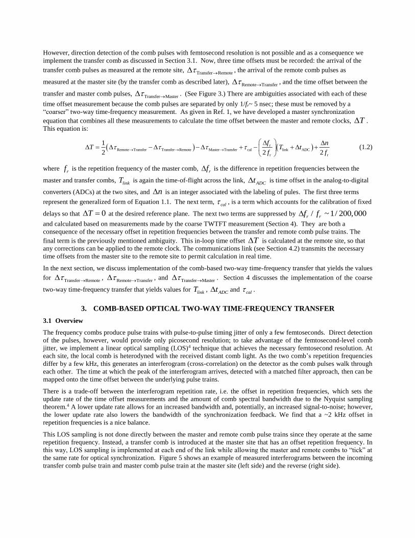
This LOS sampling is not done directly between the master and remote comb pulse trains since they operate at the same

repetition frequency. Instead, a transfer comb is introduced at the master site that has an offset repetition frequency. In

this way, LOS sampling is implemented at each end of the link while allowing the master and remote combs to “tick” at

the same rate for optical synchronization. Figure 5 shows an example of measured interferograms between the incoming

transfer comb pulse train and master comb pulse train at the master site (left side) and the reverse (right side).

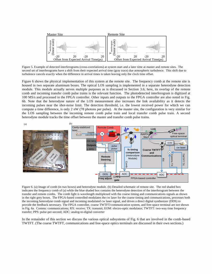
Figure 5. Example of detected interferograms (cross-correlations) at system start and a later time at master and remote sites. The

second set of interferograms have a shift from their expected arrival time (gray trace) due atmospheric turbulence. This shift due to

turbulence cancels exactly when the difference in arrival times is taken leaving only the clock time offset.

Figure 6 shows the physical implementation of this system at the remote site. The frequency comb at the remote site is

housed in two separate aluminum boxes. The optical LOS sampling is implemented in a separate heterodyne detection

module. This module actually serves multiple purposes as is discussed in Section 3.6; here, its overlap of the remote

comb and incoming transfer comb pulse trains is the relevant function. The photodetected interferogram is digitized at

100 MS/s and processed in the FPGA controller. Other inputs and outputs to the FPGA controller are also noted in Fig.

6b. Note that the heterodyne nature of the LOS measurement also increases the link availability as it detects the

incoming pulses near the shot-noise limit. The detection threshold, i.e. the lowest received power for which we can

compute a time difference, is only 2 nW (78 photons per pulse). At the master site, the configuration is very similar for

the LOS sampling between the incoming remote comb pulse train and local transfer comb pulse train. A second

heterodyne module tracks the time offset between the master and transfer comb pulse trains.

Figure 6. (a) Image of comb (in two boxes) and heterodyne module. (b) Detailed schematic of remote site. The red shaded box

indicates the frequency comb of (a) while the blue shaded box contains the heterodyne detection of the interferogram between the

transfer and remote combs. The comb light is wavelength multiplexed with the coarse timing and communications signals as shown

in the right grey boxes. The FPGA-based controlled modulates the cw laser for the coarse timing and communications, processes both

the incoming heterodyne comb signal and incoming modulated cw laser signal, and drives a direct digital synthesizer (DDS) to

provide the feedback necessary. The FPGA controller, coarse TWTFT/communication system, and free-space terminal are not shown

in Fig. 6a. Comms: communications; RX: receive; TX: transmit; EOM: electro-optic modulator; TWTFT: two-way time frequency

transfer; PPS: pulse-per-second; ADC: analog-to-digital converter

In the remainder of this section we discuss the various optical subsystems of Fig. 6 that are involved in the comb-based

TWTFT. (The coarse TWTFT, communications and free-space optics terminals are discussed in their own sections.)

-20 20-20 20

Vin

terf

ero

gra

m

(lin

ear

scal

e)

Offset from Expected Arrival Time(ps)

Master Site Remote Site

-20 20-20 20Offset from Expected Arrival Time(ps)

Vin

terf

ero

gra

m

(lin

ear

scal

e)

FPGA-based controllerFreq adjust

cw laser

EOM

+

Outputs

1 PPS

gate

1 PPS

200 MHz

Com

b

RX

Com

ms

TX

TW

TF

T T

X

ADC ADCDDS

pulse

picker

Add/Drop

filter

(Heterodyne

Module)

Link

fs timing

comparisonCoarse TWTFT

and

CommunicationsRemote

Steering

Cavity-stabilized

laser Remote Comb

(a) (b)

Free-space

optical terminal

Doppler-

cancelled link

3.2 Cavity-Stabilized Lasers and Doppler-Cancelled Links

The cavity-stabilized laser consists of a commercial cw fiber laser locked to an optical cavity yielding a ~1 Hz linewidth

and a typical environmentally-induced drift ranging from 0 Hz/s to 10 Hz/s. The cavity-stabilized laser frequency is

195.297,562 THz for the master site, and 195.297,364 THz for the remote site. The cavity-stabilized lasers are located in

an environmentally stable lab ~ 400 m away from the rooftop laboratory as the cavities are temperature sensitive. Two

separate Doppler-cancelled fiber links transport the stabilized cw light to the location of the frequency combs. The

phase-lock of the Doppler-cancelled links is monitored during synchronization to ensure that no phase slips occur.

3.3 Frequency Combs

As noted in the introduction to this section, there are three combs: a remote comb, a master comb, and a transfer comb.

All three combs are self-referenced optically-coherent fiber frequency combs with field-programmable-gate-array-based

(FPGA-based) digital control and can operate for days without any phase-slips2. The 972,920th mode of the master comb

is locked to the master cavity-stabilized laser to yield a repetition rate of ~200.733,423 MHz. The 972,909th mode of the

transfer comb is similarly locked to the same cavity-stabilized laser to yield a repetition rate that differs by

kHz. Note that the ratio / (979,920 972,909) / 972,920 r rf fD is exact and immune to clock drifts. At the remote

site, the 972,919th mode of the remote comb is locked to the second cavity-stabilized laser with an rf offset that is

ultimately adjusted for synchronization.

The comb design used here follows Ref. 2 , so the comb is actually physically distributed between two aluminum boxes,

as shown in Fig. 6a. One box contains the femtosecond fiber laser and an amplifier while a second box contains the

optics for the detection of the offset frequency (including nonlinear fiber for supercontinuum generation, periodically

poled lithium niobate for frequency doubling of the 2 m light, and in-line f-to-2f interferometer). The first aluminum

box containing the femtosecond laser is temperature controlled and both boxes are located within a larger aluminum

enclosure, as shown in Fig. 6a, which is loosely temperature controlled. This temperature control of the femtosecond

laser’s enclosure is discussed in detail in Section 3.5.

To avoid time variations due to out-of-loop fiber, the optical heterodyne signal between the frequency comb and the

cavity-stabilized laser is not detected within either of the two aluminum enclosures housing the comb. Rather the comb

light is sent to the heterodyne module (i.e. the third aluminum box in Fig. 6a), where it is finally heterodyned against the

cavity-stabilized laser to generate an error signal. This optical heterodyne signal is then sent to the comb’s FPGA digital

controller along with the offset frequency signal. The FPGA controller then phase-locks the comb output by feedback to

the femtosecond fiber laser through pump power and cavity length.

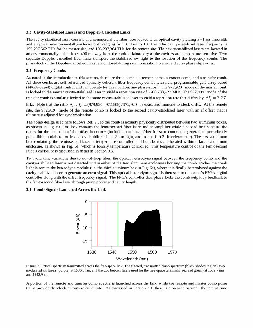
3.4 Comb Signals Launched Across the Link

Figure 7. Optical spectrum transmitted across the free-space link. The filtered, transmitted comb spectrum (black shaded region), two

modulated cw lasers (purple) at 1536.5 nm, and the two beacon lasers used for the free-space terminals (red and green) at 1532.7 nm

and 1542.9 nm.

A portion of the remote and transfer comb spectra is launched across the link, while the remote and master comb pulse

trains provide the clock outputs at either site. As discussed in Section 3.1, there is a balance between the rate of time

r 2.27fD

-15

-10

-5

0

Pow

er

(dB

)

15701560155015401530

Wavelength (nm)

offset measurements and the spectral bandwidth of the comb used for detection. It is not advantageous to try to launch

the full 1 m – 2 m octave-spanning comb spectrum across the link. Instead, as shown in Figure 7, a 16-nm-wide

optical bandwidth centered at 1555 nm out of the comb is launched across the link with a total transmitted power (at the

transmit aperture) of ~2.5 mW. The 16-nm bandwidth also leaves additional space in the C-band for the modulated cw

laser and beacon lasers without cross-talk between the comb and cw lasers.

3.5 Stabilization of the Comb against Temperature Fluctuations

Temperature control of the frequency combs is critical given their environmentally unstable location. Temperature

fluctuations cause changes in the femtosecond fiber laser cavity length and therefore the repetition frequency. To

stabilize the cavity length, the digital controller feeds back to piezo-electric transducer (PZT) actuators that are glued to

the fiber cavity. However, if the temperature excursions are too large, the resulting cavity length correction can exceed

the dynamic range of the PZTs. Their range is limited to ~ 1 m and thus the temperature of the comb must be well

controlled to within 0.1 °C - a factor of ten below that of the laboratory room temperature fluctuations.

To achieve this level of stability, 10 k thermistor is placed in good thermal contact with the inside of the enclosure

housing the femtosecond fiber laser. A commercial temperature controller then regulates the enclosure temperature via

thermo-electric coolers (TECs) placed below the aluminum enclosure. Because of temperature gradients, the thermistor

and the cavity length may not agree on the temperature so serving the cavity length by directly adjusting the temperature

is not feasible. We therefore implement a second feedback loop so that when the PZT actuator approaches the edge of its

dynamic range, the comb’s digital controller adjusts the temperature controller’s setpoint by ~ 0.05 °C increments until

the PZT actuator returns to the center of its range. This approach has an additional advantage of reduced sensitivity to

the performance characteristics of the temperature controller. We use a single point thermistor as our temperature

measurement for a dispersed set of fibers and generic Steinhart-Hart coefficients5 when computing the temperature.

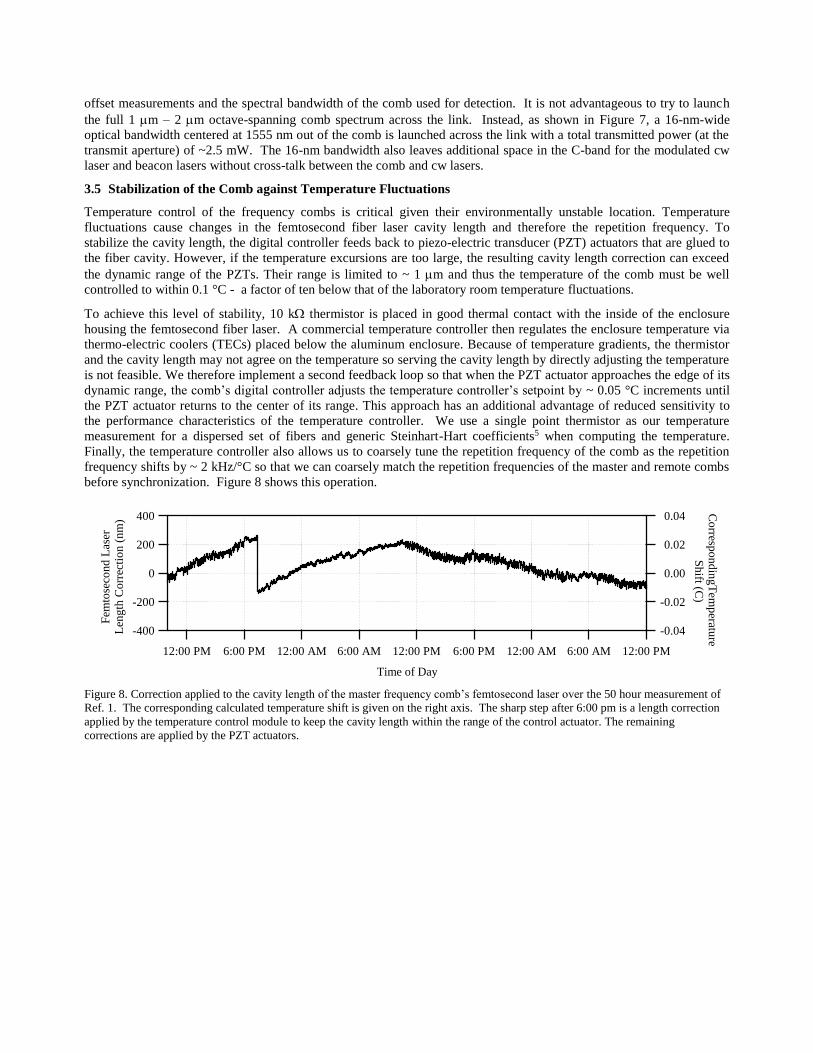
Finally, the temperature controller also allows us to coarsely tune the repetition frequency of the comb as the repetition

frequency shifts by ~ 2 kHz/°C so that we can coarsely match the repetition frequencies of the master and remote combs

before synchronization. Figure 8 shows this operation.

Figure 8. Correction applied to the cavity length of the master frequency comb’s femtosecond laser over the 50 hour measurement of

Ref. 1. The corresponding calculated temperature shift is given on the right axis. The sharp step after 6:00 pm is a length correction

applied by the temperature control module to keep the cavity length within the range of the control actuator. The remaining

corrections are applied by the PZT actuators.

-0.04

-0.02

0.00

0.02

0.04

Co

rrespo

nd

ing

Tem

peratu

re S

hift (C

)

12:00 PM 6:00 PM 12:00 AM 6:00 AM 12:00 PM 6:00 PM 12:00 AM 6:00 AM 12:00 PM

Time of Day

-400

-200

0

200

400

Fem

tose

con

d L

aser

Len

gth

Co

rrec

tio

n (

nm

)

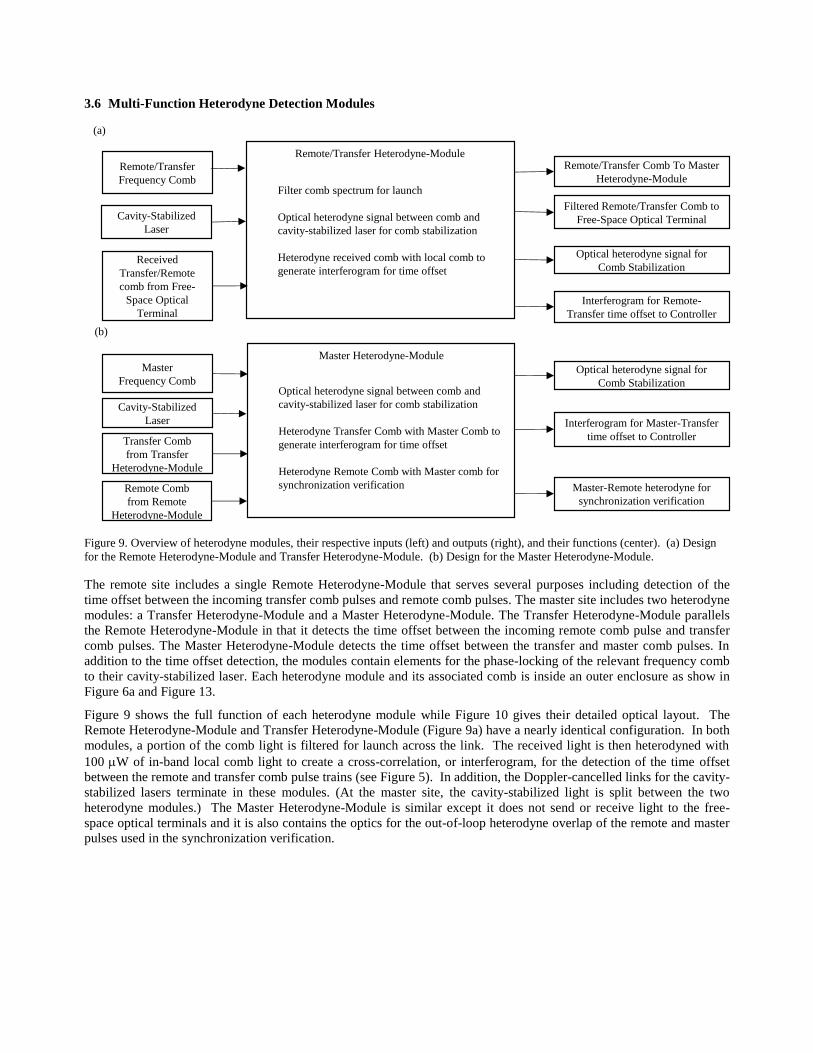
3.6 Multi-Function Heterodyne Detection Modules

Figure 9. Overview of heterodyne modules, their respective inputs (left) and outputs (right), and their functions (center). (a) Design

for the Remote Heterodyne-Module and Transfer Heterodyne-Module. (b) Design for the Master Heterodyne-Module.

The remote site includes a single Remote Heterodyne-Module that serves several purposes including detection of the

time offset between the incoming transfer comb pulses and remote comb pulses. The master site includes two heterodyne

modules: a Transfer Heterodyne-Module and a Master Heterodyne-Module. The Transfer Heterodyne-Module parallels

the Remote Heterodyne-Module in that it detects the time offset between the incoming remote comb pulse and transfer

comb pulses. The Master Heterodyne-Module detects the time offset between the transfer and master comb pulses. In

addition to the time offset detection, the modules contain elements for the phase-locking of the relevant frequency comb

to their cavity-stabilized laser. Each heterodyne module and its associated comb is inside an outer enclosure as show in

Figure 6a and Figure 13.

Figure 9 shows the full function of each heterodyne module while Figure 10 gives their detailed optical layout. The

Remote Heterodyne-Module and Transfer Heterodyne-Module (Figure 9a) have a nearly identical configuration. In both

modules, a portion of the comb light is filtered for launch across the link. The received light is then heterodyned with

100 W of in-band local comb light to create a cross-correlation, or interferogram, for the detection of the time offset

between the remote and transfer comb pulse trains (see Figure 5). In addition, the Doppler-cancelled links for the cavity-

stabilized lasers terminate in these modules. (At the master site, the cavity-stabilized light is split between the two

heterodyne modules.) The Master Heterodyne-Module is similar except it does not send or receive light to the free-

space optical terminals and it is also contains the optics for the out-of-loop heterodyne overlap of the remote and master

pulses used in the synchronization verification.

Remote/Transfer

Frequency Comb

Cavity-Stabilized

Laser

Filter comb spectrum for launch

Optical heterodyne signal between comb and

cavity-stabilized laser for comb stabilization

Heterodyne received comb with local comb to

generate interferogram for time offset

Remote/Transfer Heterodyne-Module

Optical heterodyne signal for

Comb Stabilization

Interferogram for Remote-

Transfer time offset to Controller

Remote/Transfer Comb To Master

Heterodyne-Module

Filtered Remote/Transfer Comb to

Free-Space Optical Terminal

Received

Transfer/Remote

comb from Free-

Space Optical

Terminal

Master

Frequency Comb

Cavity-Stabilized

Laser

Optical heterodyne signal between comb and

cavity-stabilized laser for comb stabilization

Heterodyne Transfer Comb with Master Comb to

generate interferogram for time offset

Heterodyne Remote Comb with Master comb for

synchronization verification

Master Heterodyne-Module

Optical heterodyne signal for

Comb Stabilization

Interferogram for Master-Transfer

time offset to Controller

Master-Remote heterodyne for

synchronization verification

Remote Comb

from Remote

Heterodyne-Module

Transfer Comb

from Transfer

Heterodyne-Module

(a)

(b)

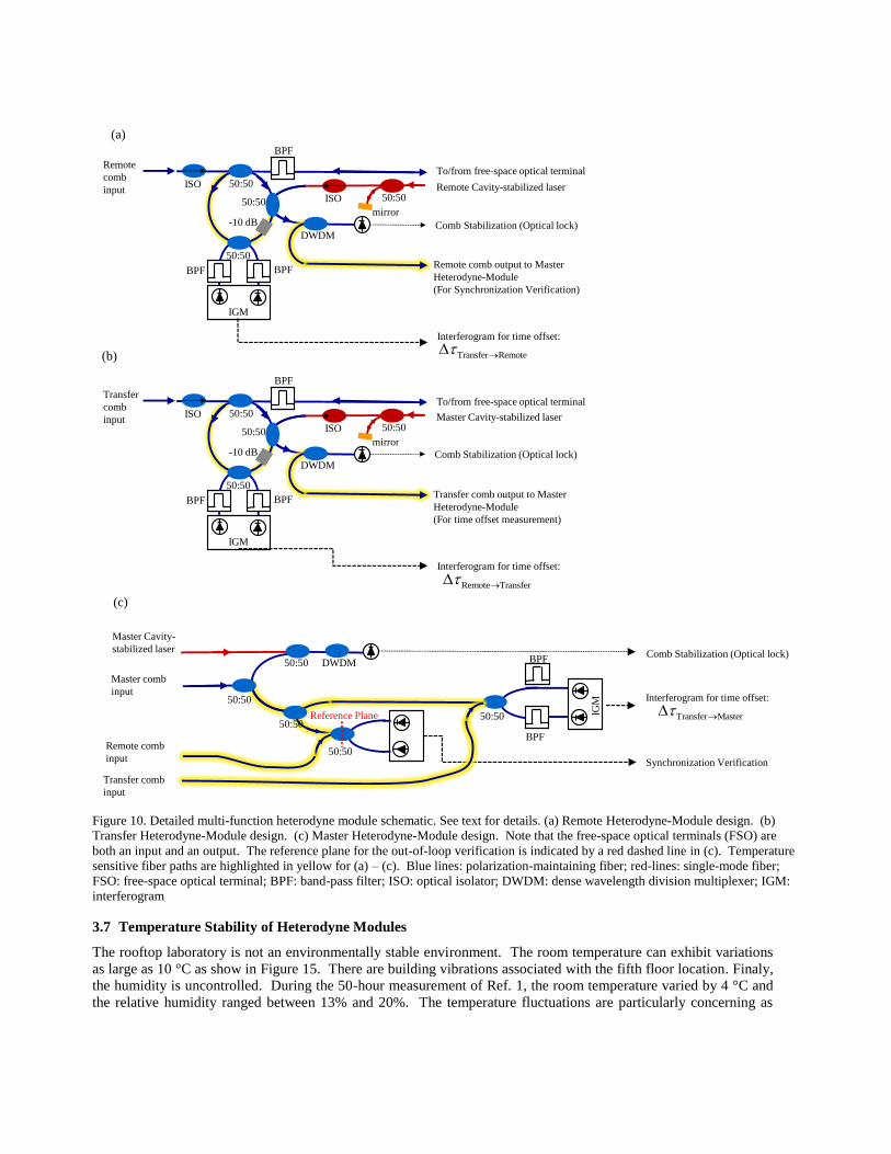
Figure 10. Detailed multi-function heterodyne module schematic. See text for details. (a) Remote Heterodyne-Module design. (b)

Transfer Heterodyne-Module design. (c) Master Heterodyne-Module design. Note that the free-space optical terminals (FSO) are

both an input and an output. The reference plane for the out-of-loop verification is indicated by a red dashed line in (c). Temperature

sensitive fiber paths are highlighted in yellow for (a) – (c). Blue lines: polarization-maintaining fiber; red-lines: single-mode fiber;

FSO: free-space optical terminal; BPF: band-pass filter; ISO: optical isolator; DWDM: dense wavelength division multiplexer; IGM:

interferogram

3.7 Temperature Stability of Heterodyne Modules

The rooftop laboratory is not an environmentally stable environment. The room temperature can exhibit variations

as large as 10 °C as show in Figure 15. There are building vibrations associated with the fifth floor location. Finaly,

the humidity is uncontrolled. During the 50-hour measurement of Ref. 1, the room temperature varied by 4 °C and

the relative humidity ranged between 13% and 20%. The temperature fluctuations are particularly concerning as

Transfer Master D

Remote Transfer D

Transfer Remote D(b)

(c)

(a)

ISO 50:50

50:50

50:50 50:50ISO

-10 dB

Remote

comb

input

To/from free-space optical terminal

Remote Cavity-stabilized laser

DWDM

mirror

Comb Stabilization (Optical lock)

IGM

Interferogram for time offset:

Remote comb output to Master

Heterodyne-Module

(For Synchronization Verification)

Master Cavity-

stabilized laser

IGM

Master comb

input

Remote comb

input

Transfer comb

input

Comb Stabilization (Optical lock)50:50 DWDM

50:50

50:50

50:50

50:50

Synchronization Verification

Interferogram for time offset:

Reference Plane

BPF

BPF BPF

BPF

BPF

ISO 50:50

50:50

50:50 50:50ISO

-10 dB

Transfer

comb

input

To/from free-space optical terminal

Master Cavity-stabilized laser

DWDM

mirror

Comb Stabilization (Optical lock)

IGM

Interferogram for time offset:

Transfer comb output to Master

Heterodyne-Module

(For time offset measurement)

BPF

BPF BPF

these fluctuations can induce fractional optical pathlength variations in fiber paths at approximately 10-5/°C. The

effect of relative humidity fluctuations is an order of magnitude lower and thus less of a concern given the usually

stable relative humidity in Boulder, Colorado. While the system includes many fiber optic paths, it has been

designed such that most fiber paths are either effectively inside the phase-locked loop for the frequency comb

stabilization or included in the bidirectional two-way link. Therefore, variations in these fiber paths do not lead to

time drifts between the synchronized clocks. However, there are a few fiber paths for which this is not the case.

These critical fiber paths are highlighted in yellow in Figure 10. To reduce temperature fluctuations on these critical

fiber paths, the heterodyne modules are housed in small aluminum boxes (see Fig. 6a), which are actively

temperature controlled at 21.0 °C with a standard deviation of 0.005 °C as measured by the control thermistor.

These boxes, along with the associated frequency comb boxes, are housed within a larger outer aluminum enclosure

that also has rough temperature control. We measured the temperature sensitivity of the synchronization by

monitoring the out-of-loop time offset while deliberating shifting the module temperature by 0.2 °C. For the Master

Heterodyne-Module, we recorded a sensitivity of 130 fs/°C, while for the Remote Heterodyne-Module and the

Transfer Heterodyne-Module, it was 100 fs/°C.

4. COARSE TWO-WAY TIME-FREQUENCY TRANSFER AND COMMUNICATIONS LINK

As discussed in Section 2.2, the comb-based TWTFT discussed in the previous section yields Transfer Remote D ,

Remote Transfer D , and Transfer Master D . However, full calculation of the time offset requires a second the coarse two-

way time-frequency transfer to provide unambiguous values for linkT ,

ADCtD and nD . In addition, the timing

information at the master site must be transmitted to the remote site. Both these functions – the measurement of the

additional timing quantities and the communications – are provided by the same physical system shown in Figure 11.

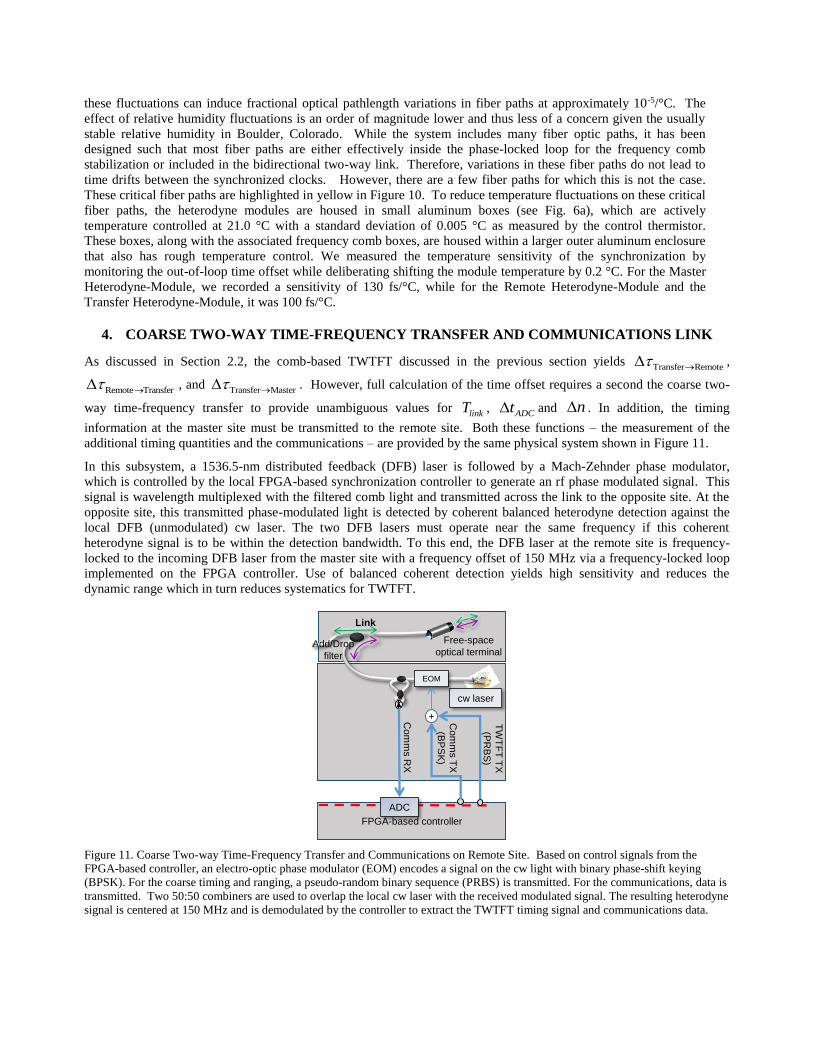
In this subsystem, a 1536.5-nm distributed feedback (DFB) laser is followed by a Mach-Zehnder phase modulator,

which is controlled by the local FPGA-based synchronization controller to generate an rf phase modulated signal. This

signal is wavelength multiplexed with the filtered comb light and transmitted across the link to the opposite site. At the

opposite site, this transmitted phase-modulated light is detected by coherent balanced heterodyne detection against the

local DFB (unmodulated) cw laser. The two DFB lasers must operate near the same frequency if this coherent

heterodyne signal is to be within the detection bandwidth. To this end, the DFB laser at the remote site is frequency-

locked to the incoming DFB laser from the master site with a frequency offset of 150 MHz via a frequency-locked loop

implemented on the FPGA controller. Use of balanced coherent detection yields high sensitivity and reduces the

dynamic range which in turn reduces systematics for TWTFT.

Figure 11. Coarse Two-way Time-Frequency Transfer and Communications on Remote Site. Based on control signals from the

FPGA-based controller, an electro-optic phase modulator (EOM) encodes a signal on the cw light with binary phase-shift keying

(BPSK). For the coarse timing and ranging, a pseudo-random binary sequence (PRBS) is transmitted. For the communications, data is

transmitted. Two 50:50 combiners are used to overlap the local cw laser with the received modulated signal. The resulting heterodyne

signal is centered at 150 MHz and is demodulated by the controller to extract the TWTFT timing signal and communications data.

FPGA-based controller

cw laser

EOM

+Com

ms

RX

Com

ms

TX

(BP

SK

)

TW

TF

T T

X

(PR

BS

)

ADC

Add/Drop

filter

Link

Free-space

optical terminal

4.1 Coarse Two-Way Time-Frequency Transfer

When the master site detects an overlap (interferogram centerburst) between the incoming remote comb pulse train and

transfer comb pulse train, it initiates the ‘coarse’ timing and communications protocol. The master side first transmits a

~104 chips Manchester-coded PRBS at ~100-ns chip length (~10 Mb/s signaling rate). The use of a Manchester-coding

allows for a simple and robust implementation. Once this signal is detected at the remote site, the remote site then

transmits its own PRBS across the link. Both sites timestamp the arrival of the local and transmitted PRBS according to

their respective local timebase. The difference of these timestamps via the analog of equation (1.1) yields the coarse time

offset between the ADC clocks, ADCtD . Since the ADCs are clocked synchronously off the remote and master combs

this measurement also yields nD . Finally, the sum of these timestamps yields the link delay linkT This PRBS-based

TWTFT has a 40 ps resolution, which is well below the 2.5 ns ambiguity which arises from the 200-MHz repetition

frequency of the combs.

4.2 Communications Link

Additionally, after the PRBS signal, the laser is modulated to communicate data between sites. For communication, the

system operates in half-duplex mode using Manchester encoded binary phase shift keying (BPSK) at 10 Mbps. The

master site uses the communication link to transmit its measured timestamps so that the remote site can use these

measurements to independently compute the coarse clock time offset and the coarse time-of-flight across the link. It also

sends the results of the comb time offset measurements. This entire protocol of PRBS two-way transfer and

communications requires 350 s of time, or below the interferogram repeat time of 1/Dfr = 500 s.

5. LOW LOSS FREE-SPACE OPTICAL TERMINALS

To provide for reciprocity through the turbulent atmosphere, a single-spatial-mode free-space link must be implemented,

essentially requiring that the phase of the received light vary by less than a radian over the receiver aperture. This

“coherence size” is a characterized property of coherent light propagating through turbulence6 and is on the order of a

few centimeters for moderate turbulence over km-scale horizontal atmospheric paths. Successful detection of the in-

loop time offset requires the received power to be above the detection threshold of a few nanowatts; increasing the

received power above this relatively low threshold does not further improve the synchronization. The free-space optical

terminals are designed to match the beam diameter to the atmospheric coherence size, to have low insertion loss in order

to support the largest range of power fluctuations possible, and to correct for turbulence-induced beam wander.

The zeroth order “piston mode” turbulence effect, given by air density variations (as well as platform sway) that change

the optical path length, is removed by the two-way time transfer as it is reciprocal for a single-spatial-mode link.

However, the first order beam wander can strongly limit link availability if uncorrected. By applying a first order tip/tilt

correction on the free-space optical terminals at both sites, we can achieve average link availabilities on average of 85%

across a 4 km link close to the ground in Boulder, Colorado.

Figure 12. Detailed schematic of low insertion loss free-space optical terminal. See text for details.

15:1 telescope

off-axis parabola

Polarization

beam combiner

Science light Beacon 1

Beacon 2

Quadrant

detector

Dichroic

Mirror

Beacon 1

1533 nm

Beacon 2

1543 nmScience

light

The terminal design is shown in Figure 12. The terminal serves to both launch light across the link and receive light

from the far end of the link, and as such are fully bi-directional. The combined ‘science’ light of the comb and

modulated cw laser is launched from single mode fiber at the input of the free-space terminal. This light is then

polarization multiplexed with a beacon laser. The beacon lasers are selected to not interfere with the science light and are

at wavelengths of 1532.7 nm and 1542.9 nm for the two terminals. (See optical spectrum in Figure 7.) The combined

beam is then directed off a fast galvanometric steering mirror, expanded in an off-axis, reflective parabolic telescope,

and launched over free space. The beacon lasers have a greater divergence than the science light in order to improve

initial signal capture but otherwise are completely co-axial with the science light. The science light has a 1/e2 diameter

of 4 cm but this is stopped down to 2.5 cm to improve light collection given the typical atmospheric coherence length

close to the ground in Boulder.

At the receiver this path is reversed; the terminal collects the received light though the telescope and directs it off the

galvanometric mirror. The received beacon is then de-multiplexed from the received science light and directed onto a

quadrant detector, while the science light is coupled into single-mode, polarization maintaining fiber which is then

connected to the heterodyne module. The dichroic mirror before the quadrant detector allows for the separation of the

incoming and outgoing beacon lasers. The signals from the quadrant detector are fed into an analog feedback system

that controls the x-y galvanometric mirror pair in order to center the beacon laser on the quad detector. With an

appropriately aligned terminal, this will also maximize the science coupled into the single mode fiber. As a consequence

of this feedback and the single-mode nature of the link, the outgoing light will be pre-aligned to the terminal at the

distant end of the link.

A first generation set of terminals exhibited 3 dB of loss per terminal. A second generation set of terminals shows a loss

of only 1.5 dB per terminal with the replacement of the parabolic reflecting telescope with a lensed telescope. The

lensed telescope has a narrower spectral coverage but can still support light across the whole C-band. As the light passes

through both terminals before detection reducing the insertion loss can greatly improve the dynamic range that can be

supported.

The total power launched at the free-space optical terminal aperture is ~ 10 mW, comprising 2.5 mW of comb power, 2.5

mW of communication/coarse timing signal power, and 5 mW of beacon power. Figure 7 shows the spectrum of the

launched light. The received comb power varies between 0 and 1 W, depending on turbulence, and can suffer

turbulence induced dropouts, i.e. the received power is below the detection threshold. The system is robust against such

dropouts, however, as most turbulence-induced dropouts are less than 10 ms in duration1.

6. VERIFICATION OF SYNCHRONIZATION

6.1 Methods of Synchronization Verification

As the 4 km link is folded back on itself via a distant mirror, a simple “out of loop” truth comparison is possible. As

show in, a ~ 1m fiber path connects the remote and master sites. (Note that all in-loop signals traverse the 4 km air

path.) The remote comb’s carrier-envelope-offset frequency is purposefully offset relative to the master carrier-envelop-

offset frequency by 1 MHz; 1 MHz is chosen for ease of demodulation. At the reference plane (red dashed line of Figure

10c), when the master and remote pulse trains overlap, we measure a 1 MHz heterodyne signal whose amplitude is

proportional to the out-of-loop time offset. After an initial calibration step, this signal yields the time offset shown in

Figure 14. As discussed below, temperature fluctuations of the ~ 1 m fiber path dominate the synchronization

verification measurement on long timescales.

Figure 13. Co-located combs allow for synchronization verification with only a short out-of-loop fiber path. (a) Schematic of the

three adjacent outer enclosures each containing a frequency comb and the associated heterodyne detection module. Critical fiber

paths are highlight in yellow. Small holes allow the critical fibers to pass between adjacent outer enclosures. Blue lines indicate

polarization-maintaining fiber. FSO: free-space optical terminal (b) Image of three adjacent outer enclosures.

An additional verification of the unambiguous synchronization of the two clocks can be performed through generation of

an optical pulse-per-second (PPS) by selecting a single pulse on each site with a Mach-Zehnder modulator (MZM).

Detection of the optical PPS can be performed with a fast photodetector and oscilloscope to verify that only one out of

2x108 pulses is present. The arrival of the remote and master optical PPS signals at a common reference plane defined at

the oscilloscope at the same time demonstrates that there are no 5-ns slips; however, the time resolution of this

verification is lower as it is limited by either the fast photodetectors or the oscilloscope.

Figure 14. Example of out-of-loop measurement of time offset between master and remote clocks demonstrating femtosecond-level

performance. Data has been down-sampled to 60 s so that the long timescale variation is more evident.

6.2 Impact of Temperature Fluctuations on Synchronization Verification

There are critical fiber paths which are not located within one of the temperature-controlled heterodyne modules,

but pass between them. These paths are highlighted in yellow in Figure 13. The first of these fiber paths conveys

the transfer comb to the master heterodyne module to measure their time offset, needed in the master

synchronization equation. The second fiber path connects the outputs of the master and remote site for

synchronization verification discussed in the previous section. (Note that this is the only connection of signals

between the master and remote site that does not pass over the 4 km free-space link even though the two sites are

adjacent in the laboratory.) Any temperature variations of these fiber paths will lead directly to time offset drifts in

the synchronization verification.

To minimize this drift, the two fiber paths have been made as short as possible by placing the enclosures adjacent to

each other with small holes drilled between them to pass the fibers. Each fiber path consists of ~ 1 m of

Remote

Comb

Transfer

CombMaster

Comb

Outer Enclosure Outer Enclosure Outer Enclosure

(a)

(b)

Remote

Heterodyne Module

Master

Heterodyne ModuleTransfer

Heterodyne Module

FSO FSO

-5

0

5

Tim

e O

ffse

t (

fs)

00:00 00:30 01:00 01:30 02:00

Elapsed Time (hh:mm)

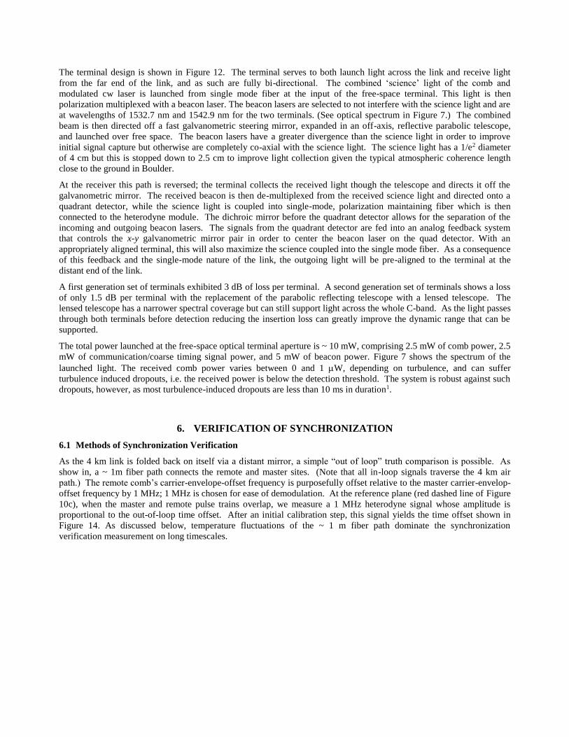
polarization-maintaining fiber. The large enclosures are temperature controlled by water-cooled breadboards affixed

to their top and bottom. As shown in Figure 15, we see a factor of 10 suppression of the external laboratory room

temperature fluctuations within these enclosures. (The slight offsets between the three enclosures should be ignored

as we use generic Steinhart-Hart coefficients5 to compute the temperature rather than calibrating each thermistor.)

The 1 °C peak-to-peak variations of Figure 15 would result in ~ 50 fs peak-to-peak variations in the delays for the 1

m fiber lengths. For Ref 1, the laboratory room temperature varied by 4 °C. Assuming the tenfold suppression

within the enclosure, we would predict a 20 fs peak-to-peak variation. Instead, we observed a factor of two larger

variation of 40 fs peak-to-peak, indicating additional contributions possibly from temperature gradients, additional

out-of-loop fiber, temperature variations of the heterodyne modules, and the impacts of relative humidity and

building vibration which are not accounted for here.

Figure 15. Suppression of laboratory room temperature fluctuations in outer enclosure. Over a two day period the laboratory showed a

10 °C variation in the room temperature (black trace). The three outer enclosures (red, blue, and orange) traces show only a 1 °C

variation over the same period.

7. CONCLUSIONS

Here we have detailed the elements of the complex optical system needed to support femtosecond-level synchronization

of clocks over turbulent air paths. While the system is not fully portable - in particular the optical cavities - there is no

fundamental limitation to implementing a portable system based on the overall design shown here.

REFERENCES [1] Deschenes, J.-D., Sinclair, L. C., Giorgetta, F. R., Swann, W. C., Baumann, E., Bergeron, H., Cermak, M.,

Coddington, I.., Newbury, N. R., “Synchronization of Distant Optical Clocks at the Femtosecond Level,”

ArXiv150907888 Phys. (2015).

[2] Sinclair, L. C., Deschênes, J.-D., Sonderhouse, L., Swann, W. C., Khader, I. H., Baumann, E., Newbury, N. R..,

Coddington, I., “Invited Article: A compact optically coherent fiber frequency comb,” Rev. Sci. Instrum. 86(8),

081301 (2015).

[3] Shapiro, J. H., “Reciprocity of the Turbulent Atmosphere,” J Opt Soc Am 61, 492–495 (1971).

[4] Coddington, I., Swann, W. C.., Newbury, N. R., “Coherent linear optical sampling at 15 bits of resolution,” Opt.

Lett. 34(14), 2153–2155 (2009).

[5] Steinhart, J. S.., Hart, S. R., “Calibration curves for thermistors,” Deep Sea Res. Oceanogr. Abstr. 15(4), 497–503

(1968).

[6] Andrews, L. C.., Phillips, R. L., Laser beam propagation through random media, 2nd ed., SPIE, Bellingham, WA

(2005).

23.7

23.5

23.3

23.1

22.9

22.7

Ou

ter

En

clo

sure

T

emp

erat

ure

(C

)

12:00 PM 12:00 AM 12:00 PM 12:00 AM 12:00 PM 12:00 AM

Time of Day

29.5

27.5

25.5

23.5

21.5

19.5

Lab

orato

ry R

oo

m

Tem

peratu

re (C)