optical sensor-based algorithm for crop nitrogen
TRANSCRIPT

Optical Sensor-Based Algorithm for CropNitrogen Fertilization*
W. R. Raun, J. B. Solie, M. L. Stone, K. L. Martin,
K. W. Freeman, R. W. Mullen, H. Zhang,J. S. Schepers, and G. V. Johnson
Department of Plant and Soil Sciences and Department of Biosystems and
Agricultural Engineering, Oklahoma State University,
Stillwater, OK, USA
Abstract: Nitrogen (N) fertilization for cereal crop production does not follow any
kind of generalized methodology that guarantees maximum nitrogen use efficiency
(NUE). The objective of this work was to amalgamate some of the current concepts
for N management in cereal production into an applied algorithm. This work at
Oklahoma State University from 1992 to present has focused primarily on the use of
optical sensors in red and near infrared bands for predicting yield, and using that infor-
mation in an algorithm to estimate fertilizer requirements. The current algorithm,
“WheatN.1.0,” may be separated into several discreet components: 1) mid-season pre-
diction of grain yield, determined by dividing the normalized difference vegetative
index (NDVI) by the number of days from planting to sensing (estimate of biomass
produced per day on the specific date when sensor readings are collected); 2) estimating
temporally dependent responsiveness to applied N by placing non-N-limiting strips in
production fields each year, and comparing these to the farmer practice (response
index); and 3) determining the spatial variability within each 0.4 m2 area using the
coefficient of variation (CV) from NDVI readings. These components are then inte-
grated into a functional algorithm to estimate application rate whereby N removal is
estimated based on the predicted yield potential for each 0.4 m2 area and adjusted
for the seasonally dependent responsiveness to applied N. This work shows that
yield potential prediction equations for winter wheat can be reliably established
with only 2 years of field data. Furthermore, basing mid-season N fertilizer rates
Received 23 December 2003, Accepted 5 October 2004*Contribution from the Oklahoma Agricultural Experiment Station.
Address correspondence to W. R. Raun, Department of Plant and Soil Sciences and
Department of Biosystems and Agricultural Engineering, Oklahoma State University,
Stillwater, OK 74078, USA. E-mail: [email protected]
Communications in Soil Science and Plant Analysis, 36: 2759–2781, 2005
Copyright # Taylor & Francis, Inc.
ISSN 0010-3624 print/1532-2416 online
DOI: 10.1080/00103620500303988
2759

on predicted yield potential and a response index can increase NUE by over 15% in
winter wheat when compared to conventional methods. Using our optical sensor-
based algorithm that employs yield prediction and N responsiveness by location
(0.4 m2 resolution) can increase yields and decrease environmental contamination
due to excessive N fertilization.
Keywords: Nitrogen rate calculator, corn, wheat, topdress nitrogen, yield based
nitrogen fertilization
INTRODUCTION
From the early 1950s to the early 1970s, increased food production was a
priority in agricultural areas around the world (Johnston 2000). During this
time period, the largest increase in the use of agricultural inputs was for
nitrogen (N) fertilizer, because it had the largest impact on yield. Since
the early 1960s, the increase in fertilizer N consumption has continued,
becoming somewhat stable over the past 10 years. Although fertilizer N
consumption and cereal grain production have both increased over the last
5 decades, contamination of surface and groundwater supplies continues
because the efficiency at which fertilizer N is used in grain production
has remained at a stagnant 33% worldwide (Raun and Johnson, 1999). While
only 33% of the nitrogen applied in fertilizer is recovered in the cereal grain
harvest, few published reports have documented practices, which significantly
improve the efficiency at which N is used in cereal production.
Voss (1998) noted that the greatest recent improvement in fertilizer
recommendations in many states was the calibration of a soil nitrate test on
which to base fertilizer N recommendations for corn (Zea mays L.).
Makowski and Wallach (2001) showed that models including end-of-winter
mineral soil N gave more profitable N fertilizer recommendations, but that
10 site-years of data were required for model parameter estimation. It should
be noted that widespread adoption of soil testing remains limited in both the
developed and developing world. In Oklahoma, annual soil testing takes
place on less than 10% of the agricultural land, and this number is
significantly less in the developing world (Hailin Zhang, Head of OSU Soil
Testing Lab, personal communication, August 2003).
Various researchers have worked to predict N mineralized from soil
organic matter, which could lead to improved N fertilizer recommendations
(Cabrera and Kissel, 1988). Recent work by Mulvaney et al. (2001) found
that the concentration of amino sugar N was highly correlated with check-
plot yields and fertilizer N response. Amino sugar N was determined on
5-g soil samples treated with 20 mL of 6 M HCl heated under reflux
(110–1208C) for 12 h. The hydrolysis mixture was then filtered and stored
at 58C. Neutralized (use of 1 M NaOH until a pH of 6.5 to 6.8 was
achieved) hydrolysates were analyzed for hydrolysable N, NH4–N, and
W. R. Raun et al.2760

amino sugar N using the diffusion methods described by Mulvaney and Khan
(2001). This methodology successfully partitioned N-responsive from non-N-
responsive corn for sites that received “normal rainfall.” It is not clear how this
technique could be implemented for within-season N fertilizer recommen-
dations, because N availability is strongly influenced by temporal changes.
Current strategies for winter wheat in Oklahoma recommend that farmers
apply 33 kg N ha21 for every 1 Mg of anticipated wheat yield (2 lb N ac21 for
every bushel of expected wheat grain yield) they hope to produce, subtracting
the amount of NO3–N in the surface (0–15 cm) soil profile (Johnson et al.,
2000). When grain yield goals are applied using this strategy, the risk of
predicting the environment (good or bad year) is placed on the producer,
especially when farmers take the risk of applying all N preplant. Schmitt
et al. (1998) reported similar recommendations of 20 kg N ha21 for every
1 Mg of corn (1.2 lb N ac21 for every bushel of corn) minus soil test
NO3–N and/or any credits from previous leguminous crops in the rotation.
To some extent, university extension (e.g., soil testing), fertilizer dealers,
and private consulting organizations have historically used grain yield
goals, due to the lack of a better alternative, and because producers have
been able to relate to an input/output strategy for computing N requirements.
Many researchers have used measurements of NO3–N in plant tissue to
identify N sufficiency or deficiency at early growth stages in winter wheat
(Vaughan et al., 1990a). However, the utility of this approach was limited
since critical tissue NO3–N levels varied as a function of temporal variability
(Raun and Westerman, 1991). Even so, petiole NO3–N has been successfully
used in potatoes, where monitoring NO3–N late in the season provided a
mechanism for improving quality in a region where irrigation was used and
temporal variability was limited (Zhang et al., 1996).
Vaughan et al. (1990b) applied a combination of improved spring fertili-
zer recommendations in winter wheat by using both total N in wheat plant
tissue and soil NH4–N to improve spring N fertilizer recommendations in
winter wheat and was able to prevent over fertilization. Work in Pennsylvania
by Fox et al. (2001) found that stalk NO3–N test taken 2 weeks after corn had
reached physiological maturity was an excellent indicator of corn N status.
A critical level of 250 mg kg21 separated N-sufficient from N-deficient
sites. This same work showed that chlorophyll meter readings at one-fourth
milk line growth stage could be used as a good indicator of corn N status,
but was less reliable if drought-stressed sites were included. In Nebraska,
Varvel et al. (1997) found that chlorophyll meter readings and end-
of-season stalk NO3-N concentrations (threshold of 2000 mg kg21) provided
additional criteria to help partition and separate fields into areas with poten-
tially different levels of residual soil N. They proposed that this information
could be used to guide soil sampling and to develop or improve site-specific
N fertilizer recommendations, which should decrease environmental risk by
reducing the amount of NO3-N available for leaching. Further inspection
of the Nebraska data showed that any time stalk nitrate levels were in the
Optical Sensor-Based Algorithm for Crop Nitrogen Fertilization 2761

250 mg kg21 region [retro evaluation versus the Fox et al. (2001) data],
grain yields were less than maximum (Gary Varvel, personal communication,
July 2003).
Wood et al. (1992) found that tissue N concentration at V10 and mid-silk
were good predictors of corn grain yield, noting that field chlorophyll
measurements using a SPAD-502 chlorophyll meter (Minolta Camera Co.,
Ltd., Japan) were highly correlated with tissue N concentrations at both of
these growth stages. Sensor work by Blackmer et al. (1994) indicated that
the measurement of light reflectance near 550 nm had promise as a technique
to detect N deficiencies in corn leaves. Varvel et al. (1997) employed chloro-
phyll meter readings to calculate a sufficiency index (as-needed treatment/well-fertilized treatment) whereby in-season N fertilizer applications were
made when index values were below 95%. If sufficiency index values were
below 90% at the V8 growth stage in corn, maximum yields could not be
achieved with in-season N fertilizer applications. This suggested that pre-
V8 N management was critical for corn.
Fiez et al. (1995) reported on the need to reduce N losses and lower N
rates in winter wheat production, especially on north-facing back-slopes.
Lengnick (1997) suggested that plant indicators followed changes in
landscape features that influenced biomass production and N uptake. He
speculated that these changes would not be revealed by soil test analyses.
Voss (1998) suggested that a regional research approach using current and
potential precision agriculture technology could provide a large and up-to-
date database on which to base nutrient recommendations across a wide
spectrum of soils and crops. This work further noted the importance of simul-
taneously using soil and plant productivity indicators to make site-specific
crop production decisions. The resolution at which these existed was not
addressed.
Raun et al. (2001) showed that yield potential could be estimated from
mid-season sensor reflectance measurements (Feekes 4 to 6) in winter
wheat. Their work employed the normalized difference vegetative index
(NDVI) computed from red and near infrared reflectance values [NDVI ¼
(NIR-Red)/(NIRþ Red)]. NIR and Red are the reflectance measurements in
the near infrared and red bands, respectively. This work predicted yield
using the sum of two post dormancy sensor readings (NDVI) divided by the
cumulative growing degree-days or GDD [(Tminþ Tmax)/2–4.48C] from
the first to the second readings. Tmin and Tmax are the minimum and
maximum temperatures in a 24-h period. Their index, in-season estimated
yield, or INSEY was later modified whereby a single NDVI measurement
was divided by the number of days from planting to sensing, counting only
those days where GDD . 0 (Raun et al., 2002). This method eliminated
those days where growth was not possible as a function of temperature,
regardless of the soil moisture conditions. Raun et al. (2002) showed that N
fertilization based on mid-season estimates of yield potential increased
NUE by more than 15% when compared to traditional practices which
W. R. Raun et al.2762

applied N at uniform rates. A significant key to the success of this work was
collecting sensor readings from each 1 m2 area and fertilizing each 1 m2,
recognizing that the differences in yield potential and subsequent fertilizer
need exists at this spatial scale. This spatial scale was determined in earlier
work, where extensive soil sampling, optical sensor measurements of plants,
and geostatistical analyses, showed that significant differences in N availabil-
ity existed at a 1 m2 spatial resolution and that each square meter needed to be
treated independently to maximize benefits (Raun et al., 1998; Solie et al.,
1999). Earlier work by Solie et al. (1996) noted that the fundamental field
element for sensing and treating fertility differences is that area which
provides the most precise measure of the available nutrient where the level
of that nutrient changes with distance.
Taylor et al. (1999) evaluated the relationship between the coefficient
of variation (CV) from grain yields and plot size. This work showed that
CV’s decreased with corresponding decreases in plot sizes. This research
suggested that the small plot sizes were consistent with the resolution where
detectable differences in soil test parameters existed and should be treated
independently. Research conducted at the International Maize and Wheat
Improvement Center (CIMMYT) suggested that the use of within row CV’s
in corn could be used to detect the physiological growth stage when
expressed spatial variability was the greatest from readings collected on a
daily basis throughout the growth cycle (Raun et al., 2005).
Over an 11-year period, the authors have developed a process to
determine N fertilizer application rate from optically sensed reflectance
measurements that vary temporally and spatially. The objective of this
paper is to describe and justify that process.
MID-SEASON NITROGEN FERTILIZATION ALGORITHM
Rationale for Basing Algorithm on Predicted Yield
In the last century, yield goals have provided one of the more reliable methods
for determining pre-plant fertilizer N rates in cereal production. The logic of
this approach makes sense, since at any given level of yield for a specific crop,
nutrient removal can be estimated based on known concentrations in each
respective grain. For example, total N concentrations in wheat, corn, and
rice grain average 2.13, 1.26, and 1.23 %N, respectively (Tkachuk, 1977).
Although there are expected differences in varieties/hybrids and growing con-
ditions, these can be accurately estimated for selected production regions and
cultivars. Once expected removal amounts are known (based on a projected
yield), mid-season application rates are determined by dividing removal by
the projected use efficiency. Similarly, known quantities of phosphorus (P),
potassium (K), sulfur (S), and other micronutrients within particular
cereal grain crops have been published by the Potash Phosphate Institute
Optical Sensor-Based Algorithm for Crop Nitrogen Fertilization 2763

(Norcross, GA) (Potash Phosphate Institute, 2000), and based on these con-
centrations, mid-season nutrient rates could be determined at specific foliar
nutrient application efficiencies.
Johnson (1991) suggested that it is usually advantageous to set the grain
yield goal above that of average yields in order to take advantage of above-
average growing conditions when they are encountered in dryland agriculture.
Dahnke et al. (1988) reported that yield goal was the “yield per acre you hope
to grow,” clearly delineating the risk farmers take when applying preplant N.
Work by Rehm and Schmitt (1989) suggested that with favorable soil moisture
at planting it would be smart to aim for a 10 to 20% increase over the recent
average when selecting a grain yield goal. They also indicated that if soil
moisture was limiting, yield goals based on past averages were not
advisable for the upcoming crop. This is an important observation, since the
strategy proposed in this paper could theoretically adjust mid-season
projected yield goal or yield potential based on soil profile moisture at
planting, or better yet, profile moisture at the time of sensing. This is consist-
ent with observations by Black and Bauer (1988) who noted that grain yield
goal should be based on how much water was available to the winter wheat
crop from stored soil water to a depth of 1.5 m in the spring plus the antici-
pated amount of growing season precipitation.
Oklahoma State University Procedure and Algorithm for
Calculating Spatial and Temporal Varying N Fertilizer Rates
The Oklahoma State University optical sensor based algorithm calculates N
fertilizer rates, and it depends on making an in-season estimate of the
potential or predicted yield, determining the likely yield response to additional
nitrogen fertilizer, and finally calculating N required to obtain that additional
yield. In addition, a procedure has been developed to modify the calculated
fertilizer response to account for the effect of spatial variation as it affects
the crop’s ability to respond to additional fertilizer. The approach of this
study was based on the ability to predict yield potential and to calculate N
required based on the total amount of a given nutrient that will be removed
in each crop.
Estimate of Yield Potential
Work by Stone et al. (1996) showed that early-season NDVI readings of
winter wheat measured with an optical sensor were highly correlated with
total above ground plant biomass. The effect of the number of days of
active plant growth prior to sensing was minimized by dividing NDVI
readings by the number of days from planting to sensing where GDD . 0.
Including only those days where GDD was more than 0 was necessary in
order to remove days where growth was not possible in winter wheat, and
W. R. Raun et al.2764

which were notably variable over sites and years. In essence, the index,
INSEY, was an estimate of biomass produced per day when growth was
possible. Raun et al. (2002) showed that optical sensor readings could be
collected once, anytime between Feekes growth stages 4 and 6, and that
INSEY was an excellent predictor of yield (grain or forage depending on
the system). This work was recently updated to include 30 locations over a
6-year period from 1998 to 2003 (Fig. 1).
What is striking from this research is that planting dates ranged from
September 24 to December 1 (difference of 68 days), and sensing dates
ranged from February 10 to April 23 (difference of 72 days), (range of differ-
ences from planting to sensing of 133 to 184 days) yet yield prediction
remained quite good (solid line). The results clearly indicated that, for
winter wheat, biomass produced per day was an excellent predictor of grain
yield. Furthermore, over this 6-year period, five different varieties
(Tonkawa, 2163, Custer, 2137, and Jagger) were included in this database
(Table 1). In this regard, it was noteworthy to find such a good relationship
with final grain yield, because so many uncontrolled variables from planting
to sensing (rainfall, planting date, temperature, etc.) had the potential to
adversely affect this relationship. The good correlation was somewhat
surprising when considering the many post-sensing stresses that could be
encountered, and would decrease yields (rust, drought, weed infestations,
etc.). These unpredictable by-site problems would undoubtedly decrease
Figure 1. Relationship between observed wheat grain yield and the In Season
Estimated Yield (INSEY) determined by dividing NDVI by the number of days from
planting to sensing (days where growth was possible, or GDD . 0) at 30 locations
from 1998 to 2003.
Optical Sensor-Based Algorithm for Crop Nitrogen Fertilization 2765

correlation, since all experimental sites were included in the database. Further-
more, considering the many post-sensing conditions that could impact the
relationship between INSEY and final grain yield, the relatively good fit of
the exponential curve in Fig. 1 (solid line) strongly supports the argument
that yield potential can indeed be predicted. However, that potential may not
be realized because post-sensing conditions could adversely impact final
grain yield.
Because of the importance of yield potential for determining N appli-
cation rates, we must expand the concept. The yield potential for any given
0.4 m2 area is the grain yield achievable, considering total plant growth
from planting, accounting for plant stand and/or damage on the date of
Table 1. Summary of planting, sensing, and harvest dates over 30 locations and 6
years
Experiment Crop cycle Planting date Sensing date Harvest date Variety
Perkins N�P 1997–98 Oct-21-97 Apr-02-98 Jun-16-98 Tonkawa
Perkins S�N 1997–98 Oct-21-97 Apr-02-98 Jun-16-98 Tonkawa
Tipton S�N 1997–98 Oct-10-97 Mar-01-98 Jun-03-98 Tonkawa
Perkins N�P 1998–99 Oct-12-98 Mar-04-99 Jun-09-99 Tonkawa
Stillwater 222 1998–99 Oct-13-98 Feb-24-99 Jun-15-99 Tonkawa
Efaw 301 1998–99 Oct-15-98 Mar-24-99 Jun-15-99 Tonkawa
Efaw AA 1998–99 Nov-9-98 Mar-24-99 Jun-15-99 Tonkawa
Haskell 801 1998–99 Oct-16-98 Mar-23-99 Jun-07-99 2163
Lahoma 502 1998–99 Oct-09-98 Mar-05-99 Jun-30-99 Tonkawa
Perkins N�P 1999–00 Oct-08-99 Feb-08-00 May-30-00 Custer
Stillwater 222 1999–00 Oct-07-99 Feb-10-00 Jul-06-00 Custer
Efaw 301 1999–00 Oct-07-99 Feb-10-00 Jun-02-00 Custer
Efaw AA 1999–00 Oct-07-99 Feb-15-00 Jul-07-00 Custer
Haskell 801 1999–00 Oct-08-99 Mar-14-00 Jun-02-00 2137
Lahoma 502 1999–00 Oct-12-99 Feb-15-00 Jun-13-00 Custer
Hennessey AA 1999–00 Oct-07-99 Feb-15-00 Jun-07-00 Custer
Perkins N�P 2000–01 Nov-17-00 Apr-13-01 Jun-07-01 Custer
Stillwater 222 2000–01 Nov-20-00 Apr-13-01 Jun-12-01 Custer
Efaw 301 2000–01 Nov-16-00 Apr-13-01 Jun-11-01 Custer
Efaw AA 2000–01 Nov-22-00 Apr-23-01 Jun-11-01 Custer
Haskell 801 2000–01 Oct-10-00 Apr-12-01 Jun-06-01 2137
Lahoma 502 2000–01 Dec-01-00 Apr-13-01 Jun-15-01 Custer
Perkins N�P 2001–02 Oct-16-01 Feb-27-02 Jun-11-02 Custer
Stillwater 222 2001–02 Oct-01-01 Feb-27-02 Jun-03-02 Custer
Efaw AA 2001–02 Oct-04-01 Feb-27-02 Jun-28-02 Custer
Haskell 801 2001–02 Oct-19-01 Mar-13-02 Jun-19-02 2137
Hennessey AA 2001–02 Oct-30-01 Mar-26-02 Jun-12-02 Custer
Stillwater 222 2002–03 Oct-14-02 Mar-12-03 Jun-23-03 Custer
Efaw AA 2002–03 Oct-05-03 Mar-10-03 Jun-23-03 Custer
Lahoma 502 2002–03 Sept-24-03 Feb-18-03 Jun-17-03 Custer
W. R. Raun et al.2766

sensing. The same spot will likely have the same yield potential whether or not
it was sensed on March 1, or March 10 for a given year, since days from
planting acts as the normalized divisor. The relationship between yield data
and sensor data can be described by an exponential curve. However,
standard regression techniques produce a prediction model that includes
data from fields whose yields were adversely affected by events subsequent
to the date of sensing that could not be predicted. Consequently, a model of
actual grain yield will under predict or over predict potential grain yield at
the sensing date. To correctly predict the potential yield, the model should
be fitted to yields unaffected by adverse conditions from sensing to
maturity. Since actual yields include some that were reduced by poor
growing conditions after sensing, and some that were not, it is important to
use the actual yields unaffected by post sensing factors when predicting
potential yield.
There is currently no established empirical method to determine how
much the curve should be shifted. We have elected to adjust the constant
‘a’ within the exponential model (y ¼ aebx) such that the number of
observations above the curve was 32% of the total data points (Fig. 1). This
curve more realistically represents the yield potential achievable in rainfed
winter wheat considering that post-sensing stresses (moisture, disease, etc.)
from February to July could lower “observed yields.” Thus, yield potential
or YP0þ 1 standard deviation is currently used in our algorithm for predicting
yield potential. The model currently used to predict wheat grain yield is:
YP ¼ 0:359 e324:4 INSEY ð1Þ
It is of further importance to note that differences from yield prediction
equations formulated using the first 2 years (1998–1999, 8 locations),
second 2 years (2000–2001, 12 locations), and third 2 years (2002–2003,
10 locations) of field data, did not differ substantially when compared to
each other (Fig. 2). This suggests that it is possible to establish reliable
yield potential prediction from only 2 years of field data, provided that
enough sites were evaluated within this time period. Regression significance
(R2) differed among the three, 2-year data sets, which was expected,
but with very small differences between regression coefficients. For all
the three, 2-year data sets, outer limits (left edge of the points from each
2-year data set moving from left to right) did not change substantially,
and the equations were quite similar to that found for the 6-year model
(Figs. 1 and 2).
Estimating the Responsiveness to Applied Nitrogen
Identifying a specific yield potential does not translate directly to an N recom-
mendation. Determining the extent to which the crop will respond to
additional N is equally important. The concept of the response index (RI)
Optical Sensor-Based Algorithm for Crop Nitrogen Fertilization 2767

was expanded from initial work by Johnson and Raun (2003) to predict crop
response to additional N fertilizer using in-season sensor measurements
(Mullen et al., 2003). The Response Index is defined as
RIHarvest ¼YldNRich
YldFieldRate
ð2Þ
where:
RIHarvest is the fertilizer Response Index for a harvested crop.
YldNRich is the grain yield from an area treated within sufficient N fertilizer to
ensure that N is non-limiting.
YldFieldRate is the grain yield from an adjacent area treated at the normal field N
application rate.
RI varied from field to field and over years and likely varied spatially
within a field. To determine RI, N fertilizer was applied to a strip extending
across a field at a rate sufficient to assure that N was not limiting, but not
excessive (Nitrogen Rich Strip). Midseason estimates of RIHarvest were
made by optically scanning the growing crop and calculating the NDVI
Figure 2. Relationship between observed wheat grain yield and the in-season-
estimated yield (INSEY) determined by dividing NDVI by the number of days
from planting to sensing (days where growth was possible, or GDD . 0) using 8
locations from 1998 to 1999, 12 locations from 2000 to 2001, and 10 locations from
2002–2003.
W. R. Raun et al.2768

response index, RINDVI:
RINDVI ¼NDVINRich
NDVIFieldRate
ð3Þ
where:
NDVINRich is NDVI of an area within the NRich strip.
NDVIFieldRate is NDVI of an adjacent area treated at the normal N rate.
This fertilizer index was developed following comprehensive work by
Johnson and Raun (2003) demonstrating that the response to applied N in
the same field is entirely variable from one year to the next and independent
of whether or not previous year yields were high or low. They studied grain
yield response to applied N in a long-term replicated experiment where the
same rates were applied to the same plots each year for over 30 years. The
response to applied N changed drastically from one year to the next, with
the check plot yield (no N applied over this 30þ year period) showing no
consistent trend to decline (Fig. 3). This was attributed to N mineralization
and variable N contributions from the atmosphere and rainfall that were unpre-
dictable over time and dependent on highly variable weather conditions
(Johnson and Raun, 2003).
Because the response to N fertilizer is dependent on the supply of non-
fertilizer N (mineralized from soil organic matter, deposited in the rainfall,
etc.) in any given year, N management strategies that include a reliable
mid-season predictor of RI should dramatically improve NUE in cereal
Figure 3. Average winter wheat grain yield from 1971 to 2003 from treatments
receiving 112 kg N ha21 annually and no fertilizer N (0 kg N ha21), long-term exper-
iment #502, Lahoma, OK. P and K applied each year to both treatments at rates of
20 and 56 kg ha21, respectively.
Optical Sensor-Based Algorithm for Crop Nitrogen Fertilization 2769

production (Johnson and Raun, 2003). This paper noted that the RI values
changed considerably when collected from the same plots that had been
managed the same way for 30 years. This was attributed to the striking differ-
ences in rainfall and temperature from one year to the next and associated
crop need (temporal variability), which influenced how much non-fertilizer
N was used by the crop.
The relationship between RI computed from NDVI readings collected
from the check plots and adequately N fertilized plots at Feekes growth
stages 4 to 6 (RINDVI) with RI computed from harvested grain (grain yield
ratio determined from the same respective plots, RIHarvest) over 63 locations
from 1998 to 2003 is reported in Fig. 4. RINDVI was positively correlated
with RIHarvest over this 6-year period. However, RINDVI could greatly underes-
timate the benefits of additional N fertilizer particularly in the middle range.
The improved fit of a linear-linear curve in this middle region indicated that
RINDVI measurements in midseason could not fully account for intervening
causes improving final yield. Despite this limitation, RINDVI has proven to be
a good, conservative predictor of wheat grain yield with additional fertilizer.
Where RINDVI is used to predict the average grain yield response to
additional fertilizer, average NDVI of the NRich strip should be compared
with average NDVI of a field rate strip immediately adjacent to the NRich
strip. Where RINDVI is used to predict spatially varying response within a
field, NDVI measurements should be made in an area where observation
indicates that response to fertilizer is high.
The highest NDVI measurement along the NRich strip can be used to
calculate Eq. (1) the maximum potential yield. YPmax is the maximum yield
Figure 4. Relationship between RINDVI and RIHarvest from 63 winter wheat exper-
iments, 1998 to 2003, central and western OK.
W. R. Raun et al.2770

that could be expected within the most productive area in a field when N was
not limiting for the year of measurement.
The boundaries circumscribing potential yield with and without
additional fertilizer are the curves predicting potential yield without additional
fertilizer (YP0), potential yield with additional fertilizer (YPN), the maximum
expected yield and a cutoff for areas with few or no wheat plants (transition
from soil to plants). The potential yield without additional fertilizer, YP0,
can be calculated directly by Eq. (1).
YP0 ¼ 0:359 e324:4 INSEY ð4Þ
The following equations predict the potential yield with additional N fertilizer,
YPN:
YPN ¼ YP0�RINDVI NDVIFieldRate � 0:25 and YPN , YPmax ð5aÞ
or
YPN ¼ YPmax YP0�RINDVI � YPmax ð5bÞ
Observations over several years indicate that values of NDVI , 0.25 occur on
bare soil or on soil with wheat stands so poor at Feekes 5 that they will not
produce appreciable yields.
Examination of Fig. 5 illustrates the critical points of the RI theory for
predicting yield increase. Below field rate NDVI ¼ 0.25, when measured
after 120 days of active plant growth, crop potential yield is considered
low enough that there are no appreciable benefits in adding additional N.
This is the transition from bare soil to wheat. In this example, between
NDVI ¼ 0.25 and NDVI ¼ 0.57 the crop benefits from additional N, and
the potential yield increase is the product of RI and potential yield without
Figure 5. Change in potential yield of wheat with additional N fertilizer for
a Response Index of RI ¼ 1.5, a maximum potential yield of 3.0 Mg ha21 and
120 days after planting where GDD . 0.
Optical Sensor-Based Algorithm for Crop Nitrogen Fertilization 2771

additional N, YP0. Between NDVI ¼ 0.57 and NDVI ¼ 0.73, additional ferti-
lizer can boost grain yield up to the maximum potential yield, YPmax. Beyond
NDVI ¼ 0.73 there is no benefit for additional fertilizer N, because potential
yields have reached the maximum for the field.
The RI theory for predicting yield increase with additional N has
one additional consequence. Increasing the value of RI causes YPN to more
rapidly reach YPmax (Fig. 6). This causes the division point separating
the region where the response index controls YPN from the region where
YPmax limits YPN to shift to lower values of NDVI. At its extreme, where
RINDVI ¼ 4.3, the crop yield at any location in the field and NDVI � 0.25
can be raised to the maximum yield.
The topdress N requirement can be calculated by
R ¼ 23:9YPN � YP0
hð7Þ
where: R is the N application rate, kg/ha; 23.9 is the decimal percentage of N
by weight contained in wheat grain multiplied by a conversion constant h is an
efficiency factor, 0.5 � h � 0.7.
Plots of Eq. (7) for response indices of 1.25, 1.75, and 2.5 illustrate the
effect of the RI on the nitrogen application rate (Fig. 7). The maximum N appli-
cation rate for RI ¼ 1.25 was 23.7 kg ha21, and the peak value did not occur
until the field rate NDVI reached 0.70. As RI increased to 2.5, the peak N appli-
cation rate increased to 72.4 kg ha21, and the peak application rate occurred
at a much lower value of field rate NDVI, 0.45. For the conditions of
YPmax ¼ 3 Mg ha21 and 120 days after planting where GDD . 0, RI would
equal 4.3, the N application rate equals 92.9 kg ha21, and the peak application
rate occurs at NDVI equals 0.25. In that case, only N is the limiting factor.
Figure 6. Shift in portion of the YPN curve for changes in the Response Index,
RI, where YPmax serves as the upper boundary for potential yields from additional N
fertilizer for a maximum potential yield of 3.0 Mg ha21 and 120 days after planting
where GDD . 0.
W. R. Raun et al.2772

Validation of the Oklahoma State University Optical Sensor-Based
Algorithm for Crop Nitrogen Fertilization occurs at two levels, paired com-
parisons of estimated yield from NRich and adjacent field rate fertilizer
strips and an extensive series of field trials testing the algorithm. Earlier this
year, 16 NRich strips sensed with either the GreenSeekerTM sensor or
IKONIS satellite imagery were examined. For the IKONIS imagery, NDVI
was calculated for paired pixels in the NRich strip and the adjacent field
rate area. Pixel size was 4 by 4 m and paired data were separated by one
pixel, 4 m. An examination of the data compared with the imagery showed
that aberrations in the form of spikes in RINDVI occurred whenever the
NRich strip crossed a terrace. These spikes occurred because of the relatively
large pixel size and the fact that data pairs were separated by 4 m and NDVI
values changed between the backside and channel of the terraces. The result
was no relatedness between “paired” measurements. Data in the vicinity of
terraces were deleted. Potential yield was calculated for data from the
NRich strip. YPNRich data were plotted in Fig. 8 along with the YP0, YPN,
YPmax and Soil/Plant transition curves as a function of field rate NDVI.
The YPN curve was calculated using the maximum value of RINDVI along
the strip, RINDVI ¼ 1.37.
All data fell on or below the YPmax cap, but NRich potential yield data
paired with field rate NDVI measurements �0.52 were clustered closely
in the vicinity of the cap. The few measurements falling below the YP0
boundary were a consequence of the limited relatedness that could occur
when measurements separated by 4 m were use to calculate RINDVI. In these
instances, RINDVI ,1. As noted previously, RINDVI provided a conservative
estimate of NDVI with a number of YPNRich data points paralleling the YPN
curve but with values greater than predicted by RINDVI. To overcome the
problem of underestimating potential yield, an alternative response index
Figure 7. N application rate required to maximize wheat grain yield calculated using
the “Optical Sensor-Based Algorithm for Crop Nitrogen Fertilization Optimization”
for three response indices and 3.0 Mg ha21 maximum potential yield, YPN, and
120 days after planting where GDD . 0.
Optical Sensor-Based Algorithm for Crop Nitrogen Fertilization 2773
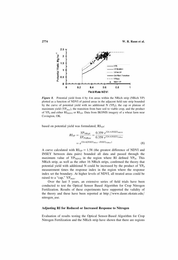
based on potential yield was formulated, RIYP:
RIYP ¼YPNRigh
YPFldRate
¼0:359 e324:4 INSEYNRICH
0:359 e324:4 INSEYFldRate
¼ e324:4ðINSEYNRich�INSEYFldRateÞ ð8Þ
A curve calculated with RIYP ¼ 1.58 (the greatest difference of NDVI and
INSEY between data pairs) bounded all data and passed through the
maximum value of YPNDVI in the region where RI defined YPN. This
NRich strip, as well as the other 16 NRich strips, confirmed the theory that
potential yield with additional N could be increased by the product of YP0
measurement times the response index in the region where the response
index set the boundary. At higher levels of NDVI, all treated areas could be
raised to a “cap,” YPmax.
Over the last 5 years, an extensive series of field trials have been
conducted to test the Optical Sensor Based Algorithm for Crop Nitrogen
Fertilization. Results of these experiments have supported the validity of
the theory and these have been reported at http://www.dasnr.okstate.edu/nitrogen_use.
Adjusting RI for Reduced or Increased Response to Nitrogen
Evaluation of results testing the Optical Sensor-Based Algorithm for Crop
Nitrogen Fertilization and the NRich strip have shown that there are regions
Figure 8. Potential yield from 4 by 4 m areas within the NRich strip (NRich YP)
plotted as a function of NDVI of paired areas in the adjacent field rate strip bounded
by the curve of potential yield with no additional N (YP0), the cap or plateau of
maximum yield (YPmax), the transition from bare soil to viable crop, and the product
of YP0 and either RINDVI or RIYP. Data from IKONIS imagery of a wheat farm near
Covington, OK.
W. R. Raun et al.2774

in the field where the response to additional N is less than or occasionally
greater than predicted by the algorithm.
Measuring the variability in plant stand and growth at high resolution,
less than 0.4 m2, in farmer fields can enable us to adjust the response
index for mid-season N fertilization in grain crops. In general, this small
area spatial variability can be estimated by the coefficient of variation
(CV) of high-resolution measurements of NDVI. CV has been shown to be
highly correlated with plant population within each 0.4 m2 area. NDVI is
well correlated with N uptake (Stone et al., 1996), and since N uptake is
the product of N content and plant biomass (plant population), it follows
that estimates of N uptake will be improved by identifying changes in
plant population and plant growth. Because of this relationship, more can
be deciphered about the potential yield obtainable with added N fertilization
than by an average value of NDVI within the sensed and treated area. If
plant stands and growth are irregular (high CV), the potential yield with
added N fertilization, RI, will be lower than if plant stands are uniform
(low CV) with the same mean NDVI. On-the-go monitoring of the NDVI
coefficient of variation offers the potential to improve our calculation of N
fertilizer rate.
The ability to accurately measure CV’s on-the-go is also a function of
the sensors employed. The sensors developed by Oklahoma State University
and currently sold by NTech Industries (Ukiah, CA) collect many individual
readings (.10 in each 0.4 m2 traveling at 10 mph). No other precision
agricultural technology being developed today can collect as many compre-
hensive readings on such a small scale, and on-the-go. Work by Taylor et al.
(1997) indicated that 15 to 16 readings from each area of interest were
required to obtain a reliable composite soil sample. The 10 readings
collected from each 0.4 m2 used here were considered to be sufficient to
obtain a composite sample from such a small area, understanding that
the 10 sensor readings were representative of each 0.4 m2 surface
area. The resultant CV from the area of interest is representative of
the variability from the same 0.4 m2 area, not just a small portion as
would be the case with chlorophyll meters. Clearly, plant stands should be
expected to vary at the same scale for which they are planted, which is by
seed in corn.
Over the last 2 years, high-frequency measurements of NDVI were
made and wheat yields collected at 1 m2 resolution (Fig. 9). These data
show a definite relationship between CV within a plot and grain yield,
despite the scatter in data. An Eq. (9) relating the response index to the
coefficient of variation can be derived the linear model for CV – wheat
yield data:
YPCV ¼ �0:0399CV � 3:3736 ð9Þ
Optical Sensor-Based Algorithm for Crop Nitrogen Fertilization 2775

Dividing by the average yield at CV ¼ 0, YPCV0 gives:
YPCV
YPCV0
¼ �0:01219CV þ 1
YPCV=YP0
YPCV0=YP0
¼RICV
RICV0
¼ �0:01219CV þ 1
RICV ¼ RICV0ð�0:01219CV þ 1Þ ð10Þ
When measured in the field, NDVIFldRate always has a CV . 0. Equation (11)
can be used to calculate the intercept RICV0:
RICV0 ¼RIMax
�0:1219CVMaxRI
ð11Þ
where RIMax is the maximum response index along the NRich strip and
CVMaxRI is the CV of the field rate NDVI used to calculate RIMax. Predicted
yield using RICV, YPCV, is calculated by Eq. (12):
YPCV ¼ RICV YP0 ð12Þ
These equations hold for RINDVI, RIYP, or any other response index predicting
increased yield with additional fertilizer N. The effect of CV on the response
index is similar to that seen with changes in measured RI (Fig. 10). Although
CV of wheat used to calculate YPmax is generally very low, there can be
instances when yields predicted using RICV are greater than YPmax.
Figure 9. Relationship between observed grain yield and the coefficient of variation
from sensor readings taken at early stages of growth (Feekes 4 to 6) in winter wheat
from 21 locations over a 3-year period, 2000–2003.
W. R. Raun et al.2776

DISCUSSION
If the resolution where significant differences in biological properties (plant or
soil) were found at 0.4 m2, that same resolution would be where recognizable
differences in statistical properties could be discerned as well. Nutrients can
vary at different scales for different reasons. Variability at the finest scale
encompasses all causes. At coarser scales, we average out some of the
cause for variability. Spatial variability of soil nutrients has already been
established for a resolution scale of 0.4 m2. Therefore, variability among
0.4 m2 areas is a function of nutrient availability, whereas variability within
0.4 m2 is likely a function of crop conditions other than nutrient availability.
Furthermore, it should be noted that plants and their roots integrate nutrient
variability that can exist within each 0.4 m2, but that is not expressed
because plant uptake and/or growth will average whatever variability might
be present at that scale.
Although CVs from small yield potential plots assisted in removing some
of the variation in predicted yield when combined with INSEY (in season
estimated yield), this approach is flawed since the CV needs to be applied
to the response index for added N fertilization. Adjusting RI as a function
of CV can account for the inability to reach the yield predicted by RI or
maximum potential yield, YPmax.
The yield potential obtainable without added N fertilization (YP0) for a
minimum sized field element should be independent of CV. This was
confirmed when evaluating the relationship between CV determined from
NDVI readings taken between Feekes 4 and 6 over 21 locations from 2000
to 2003, and where yield data were also collected from 1 m2 areas (Fig. 6).
Although there was a trend for grain yields to decrease with increasing CV,
correlation was poor.
Unlike YP0, the yield potential obtainable with added N fertilization
(YPN) should be dependent on CV. While actual yield level with no added
Figure 10. The effect of CV of high-resolution NDVI measurements on the response
index and potential wheat yield.
Optical Sensor-Based Algorithm for Crop Nitrogen Fertilization 2777

inputs is independent of CV, the yield level that can be achieved if changes or
additions are made is directly related to how much the level of variability
existed within each 0.4 m2 area. When CV is low, a responsive field
element should be capable of greater yield than when a similarly responsive
field element CV is large. To test this concept, observed grain yield
obtained when added N fertilization occurred after sensing was evaluated as
a function of predicted yield using INSEY and the coefficient of variation at
the time of sensing in the equation (YPN_CV). Predictive methods for deter-
mining YPN_CV were delineated in the previous section. For all the plots
reported in Fig. 7, NDVI sensor readings were taken from winter wheat
somewhere between Feekes growth stages 4 and 6. Enough readings were
collected from each plot to determine the CV. Following sensor readings, N
was applied at different rates (varied by location and year) to achieve the
yield potential estimated in the RI-NFOA algorithm. CV data were not used
to determine N application rates. To evaluate the potential usefulness of CV
for predicting the yield that could be achieved with added N fertilization,
actual yield, YPN and YPN_CV were plotted for all 6 trials where these data
were collected (Fig. 11). YPN clearly resulted in overestimating actual
yields obtained, 5.5 Mg ha21. YPN_CV values more closely followed
observed yield. When actual INSEY values exceed 0.006, observed yield
clearly reached a plateau or yield maximum of 3.0 Mg ha21. Although the
Figure 11. Relationship between observed grain yield and in-season-estimated-yield
(INSEY, NDVI divided by the # of days from planting to sensing where growing
degree days were greater than 0), including the predicted yield that could be obtained
with added N fertilization (YPN ¼ INSEY or YP0 times the response index) and YPN
as a function of the coefficient of variation YPN_CV from six trials where added N
fertilization was received after sensing.
W. R. Raun et al.2778

current YPN_CV formula employed resulted in a plateau at somewhat higher
INSEY values (0.008) than with observed yield (0.006), it predicted a yield
plateau.
The need to sense biological properties on a small scale (0.4 m2 or
smaller) was established by Solie et al. (1999). Not until recently did we
consider the evaluation of statistical properties within each 0.4 m2, under-
standing that the variability within each 0.4 m2 would be associated with
something other than nutrient variability that would be minimal at this
scale. Fortunately, the sensors developed and used in all the Oklahoma
State University Sensor research are capable of collecting enough data
within each 0.4 m2 to calculate meaningful statistical estimates at this small
scale. Now, these statistical estimates on each 0.4 m2 can be combined with
average NDVI from the same 0.4 m2 to better predict mid-season yield and
subsequent fertilizer N rate requirements. Using the RI-NFOA algorithm
reported earlier, Raun et al. (2002) showed that winter wheat NUE was
improved by more than 15% when N fertilization was based on INSEY
calculated from optically sensed NDVI, determined for each 1 m2 area, and
the response index when compared to traditional practices at uniform N
rates. We are not aware of any biological basis to suggest that this approach
would not be suitable in other cereal crops.
REFERENCES
Black, A.L. and Bauer, A. (1988) Setting winter wheat yield goals. In Central GreatPlains Profitable Wheat Management Workshop Proceedings; Havlin, J.L., ed.;Potash & Phosphate Institute: Atlanta, Georgia.
Blackmer, T.M., Schepers, J.S., and Varvel, G.E. (1994) Light reflectance comparedwith other nitrogen stress measurements in corn leaves. Agronomy Journal, 86:934–938.
Cabrera, M.L. and Kissel, D.E. (1988) Evaluation of a method to predict nitrogenmineralized from soil organic matter under field conditions. Soil Science Societyof America Journal, 52: 1027–1031.
Dahnke, W.C., Swenson, L.J., Goos, R.J., and Leholm, A.G. (1988) SF-822. InChoosing a Crop Yield Goal; North Dakota State Extension Service: Fargo, NorthDakota.
Fiez, T.E., Pan, W.L., and Miller, B.C. (1995) Nitrogen use efficiency of winterwheat among landscape positions. Soil Science Society of America Journal, 59:1666–1671.
Fox, R.H., Piekielek, W.P., and Macneal, K.E. (2001) Comparison of late-season diag-nostic tests for predicting nitrogen status of corn. Agronomy Journal, 93: 590–597.
Johnson, G.V. (1991) General model for predicting crop response to fertilizer.Agronomy Journal, 83: 367–373.
Johnson, G.V. and Raun, W.R. (2003) Nitrogen response index as a guide to fertilizermanagement. Journal of Plant Nutrition, 26: 249–262.
Johnson, G.V., Raun, W.R., Zhang, H., and Hattey, J.A. (2000) Soil Fertility Handbook;Oklahoma Agricultural Experiment Station: Stillwater, Oklahoma, 61–64.
Optical Sensor-Based Algorithm for Crop Nitrogen Fertilization 2779

Johnston, A.E. (2000) Efficient use of nutrients in agricultural production systems.
Communications in Soil Science and Plant Analysis, 31: 1599–1620.
Lengnick, L.L. (1997) Spatial variation of early season nitrogen availability indicators
in corn. Communications in Soil Science and Plant Analysis, 28: 1721–1736.
Makowski, D. and Wallach, D. (2001) How to improve model-based decision rules for
nitrogen fertilization. European Journal of Agronomy, 15: 197–208.
Mullen, R.W., Freeman, K.W., Raun, W.R., Johnson, G.V., Stone, M.L., and Solie, J.B.
(2003) Identifying an in-season response index and the potential to increase wheat
yield with nitrogen. Agronomy Journal, 95: 347–351.
Mulvaney, R.L. and Khan, S.A. (2001) Diffusion methods to determine different forms
of nitrogen in soil hydrolysates. Soil Science Society of America Journal, 65:
1284–1292.
Mulvaney, R.L., Khan, S.A., Hoeft, R.G., and Brown, H.M. (2001) A soil organic
nitrogen fraction that reduces the need for nitrogen fertilization. Soil Science
Society of America Journal, 65: 1164–1172.
Potash Phosphate Institute. (2000) In Plant Food Uptake for Great Plains Crops;
Potash Phosphate Institute: Norcross, Georgia.
Raun, W.R. and Johnson, G.V. (1999) Improving nitrogen use efficiency for cereal
production. Agronomy Journal, 91: 357–363.
Raun, W.R. and Westerman, R.L. (1991) Nitrate-N and phosphate-P concentration in
winter wheat at varying growth stages. Journal of Plant Nutrition, 14: 267–281.
Raun, W.R., Johnson, G.V., Stone, M.L., Solie, J.B., Lukina, E.V., Thomason, W.E.,
and Schepers, J.S. (2001) In-season prediction of potential grain yield in winter
wheat using canopy reflectance. Agronomy Journal, 93: 131–138.
Raun, W.R., Solie, J.B., Johnson, G.V., Stone, M.L., Mullen, R.W., Freeman, K.W.,
Thomason, W.E., and Lukina, E.V. (2002) Improving nitrogen use efficiency in
cereal grain production with optical sensing and variable rate application.
Agronomy Journal, 94: 815–820.
Raun, W.R., Solie, J.B., Johnson, G.V., Stone, M.L., Whitney, R.W., Lees, H.L.,
Sembiring, H., and Phillips, S.B. (1998) Micro-variability in soil test, plant nutrient,
and yield parameters in bermudagrass. Soil Science Society of America Journal, 62:
683–690.
Raun, W.R., Solie, J.B., Martin, K.L., Freeman, K.W., Stone, M.L., Johnson, G.V., and
Mullen, R.W. (2005) Growth stage, development, and spatial variability in corn
evaluated using optical sensor readings. Journal of Plant Nutrition, 28 (1): in press.
Rehm, G. and Schmitt, M. (1989) Minnesota Extension Service, University of
Minnesota. In Setting realistic crop yield goals; St. Paul: Minnesota, AG-FS-3873.
Schmitt, M.A., Randall, G.W., and Rehm, G.W. (1998) University of Minnesota
Extension Service. In A soil nitrogen test option for N recommendations with
corn; St. Paul: Minnesota, FO-06514-GO.
Solie, J.B., Raun, W.R., and Stone, M.L. (1999) Submeter spatial variability of selected
soil and bermudagrass production variables. Soil Science Society of America
Journal, 63: 1724–1733.
Solie, J.B., Raun, W.R., Whitney, R.W., Stone, M.L., and Ringer, J.D. (1996) Optical
sensor based field element size and sensing strategy for nitrogen application. Trans.
ASAE, 39 (6): 1983–1992.
Stone, M.L., Solie, J.B., Raun, W.R., Whitney, R.W., Taylor, S.L., and Ringer, J.D.
(1996) Use of spectral radiance for correcting in-season fertilizer nitrogen
deficiencies in winter wheat. Trans. ASAE, 39 (5): 1623–1631.
W. R. Raun et al.2780

Taylor, S.L., Johnson, G.V., and Raun, W.R. (1997) A field exercise to acquaintstudents with soil testing as a measure of soil fertility status and field variability.Journal of Natural Resources Life Sci. Educ., 26: 132–135.
Taylor, S.L., Payton, M.E., and Raun, W.R. (1999) Relationship between mean yield,coefficient of variation, mean square error and plot size in wheat field experiments.Communications in Soil Science and Plant Analysis, 30: 1439–1447.
Tkachuk, R. (1977) Calculation of the nitrogen-to-protein conversion factor. InNutritional Standards and Methods of Evaluation for Food Legume Breeders;Hulse, J.H., Rachie, K.O. and Billingsley, L.W., eds.; International DevelopmentResearch Centre: Ottawa, Canada., 78–82.
Varvel, G.E., Schepers, J.S., and Francis, D.D. (1997) Ability for in-season correctionof nitrogen deficiency in corn using chlorophyll meters. Soil Science Society ofAmerica Journal, 61: 1233–1239.
Varvel, G.E., Schepers, J.S., and Francis, D.D. (1997) Chlorophyll meter and stalknitrate techniques as complementary indices for residual nitrogen. Journal ofProd. Agric., 10: 147–151.
Vaughan, B., Barbarick, K.A., Westfall, D.G., and Chapman, P.L. (1990a) Tissuenitrogen levels for dryland hard red winter wheat. Agronomy Journal, 82: 561–565.
Vaughan, B., Westfall, D.G., Barbarick, K.A., and Chapman, P.L. (1990b) Springnitrogen fertilizer recommendation models for dryland hard red winter wheat.Agronomy Journal, 82: 565–571.
Voss, R. (1998) Fertility recommendations: past and present. Communications inSoil Science and Plant Analysis, 29: 1429–1440.
Wood, C.W., Reeves, D.W., Duffield, R.R., and Edmisten, K.L. (1992) Fieldchlorophyll measurements for evaluation of corn nitrogen status. Journal of PlantNutrition, 15: 487–500.
Zhang, H., Smeal, D., Arnold, R.N., and Gregory, E.J. (1996) Potato nitrogenmanagement by monitoring petiole nitrate level. Journal of Plant Nutrition,19: 1405–1412.
Optical Sensor-Based Algorithm for Crop Nitrogen Fertilization 2781