LLNL-PRES-694059This work was performed under the auspices of the U.S. Department of Energy by Lawrence Livermore National Laboratory under contract DE-AC52-07NA27344. Lawrence Livermore National Security, LLC

Optical Ranging Overview and Analysis of Calibration Data

PDV Workshop 2016

Natalie Kostinski (LLNL),Brandon La Lone (NSTec), Corey Bennett (LLNL), Marylesa Howard

(NSTec), Adam Lodes (LLNL), Bruce Marshall (NSTec)

June 9, 2016

LLNL-PRES-6940592

“Not with a Bang But a Chirp”Barney Oliver (Bell Labs)

Memorandum on high-power radar pulses

“This is the way the world ends. Not with a bang but a whimper.” –T.S. Eliot

LLNL-PRES-6940593

What is a chirp?

• A chirp is a signal in which the frequency increases or decreases with time• In this talk, we mostly care about linear chirps:

Time Domain Frequency Domain

Quadratic Phase

LLNL-PRES-6940594

What is Optical Ranging (OR)?

OR is a fast interferometric technique used to measure distance to a target at periodic intervals

Spectral interferometer: — light pulses in target and reference arms interfere — chromatic dispersion in the fiber maps spectral information

into the time domain (real-time dispersive Fourier transformation)

— beat waveform is recorded

Also known as “Broadband Laser Ranging” (BLR)

LLNL-PRES-6940595

Schematic of current setup

Fiber converts the interference spectrum into the time domain via real-time dispersive Fourier transformation

A

B

C

LLNL-PRES-6940596

Idealized frequency domain description demonstrates the insensitivity to Doppler shift

DopplerTime Delay

After Linear Dispersion

Time (t)

Targ

et

Ref

Time Delay = Beat freq/(dF/dt)Position = c*Time Delay/2

Inte

nsity

Time Delay

Beat: Electrical Waveform

Opt

ical

Fre

quen

cy (F

)

B C

Doppler

LLNL-PRES-6940597

Chirped signals

The chirp is due to Third Order Dispersion (TOD) in fiber

Time Delay

After Nonlinear DispersionTa

rget

Ref

Time Delay

Opt

ical

Fre

quen

cy

Time

Inte

nsity

Beat: Electrical Waveform

Doppler

Beat Freq

B C

Doppler

LLNL-PRES-6940598

Calibration before experiment

The calibration establishes a correction for dechirping the beat waveform, and a relation between beat frequency and distance

LLNL-PRES-6940599

Example calibration files

It is the beat frequency that we care about...this will correspond to a particular distance to target

We also care about what we call the pulse edge or start time

Near balance point of interferometer

LLNL-PRES-69405910

Analysis steps for calibration data

Collect data at different distances (5 Pulses each at 41 distances)

For every pulse,— Find envelope and subtract— Estimate the phase— Dechirp the signal— Find frequency of dechirped signal

Do a linear least squares fit of signal beat frequency vs distance to get a slope – the correction to be applied to experimental data

LLNL-PRES-69405911

Envelope detection

For a particular distance file— Find the envelope and subtract from original signal

LLNL-PRES-69405912

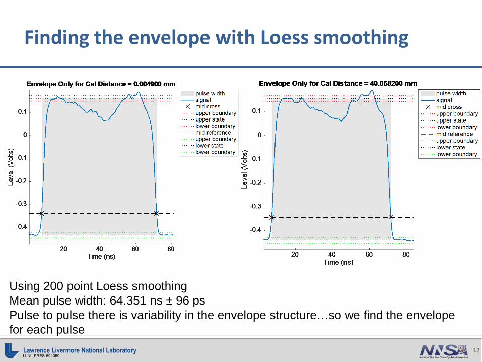
Finding the envelope with Loess smoothing

Using 200 point Loess smoothingMean pulse width: 64.351 ns ± 96 psPulse to pulse there is variability in the envelope structure…so we find the envelope for each pulse

LLNL-PRES-69405913

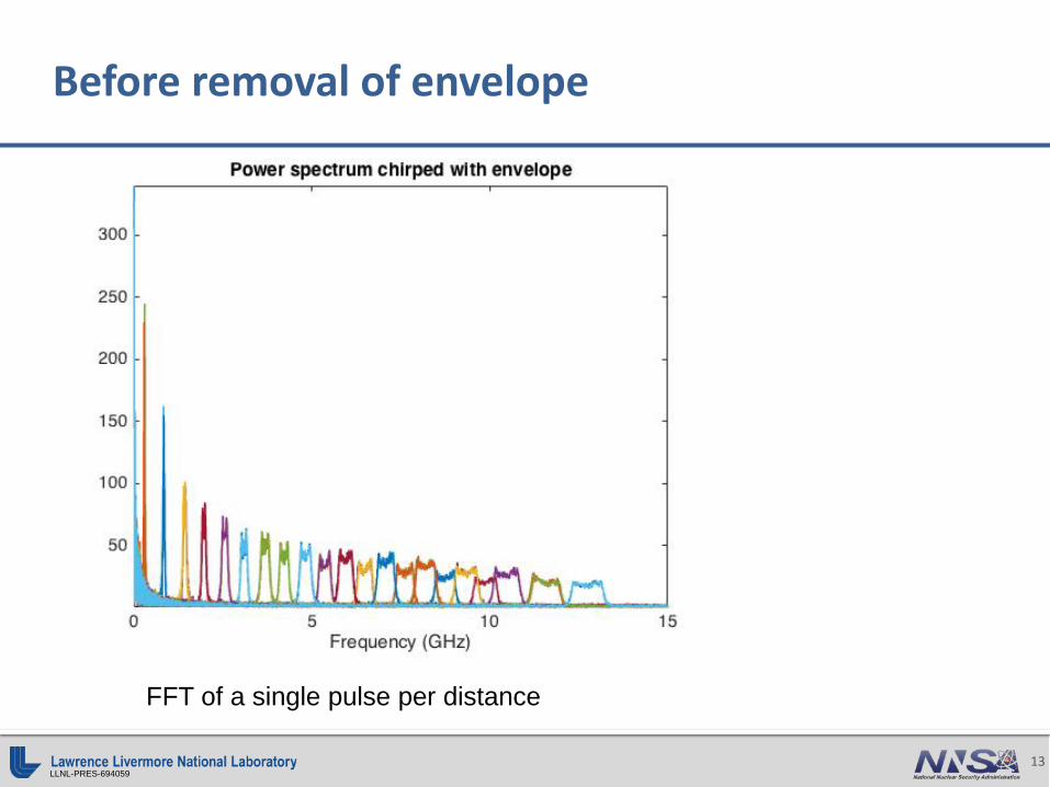
Before removal of envelope

FFT of a single pulse per distance

LLNL-PRES-69405914

Before removal of envelope: a closer look

Baseband…the envelope information

Signals we care about at 4 different distances

LLNL-PRES-69405915

After removal of the envelope

Envelope removed

LLNL-PRES-69405916

Finding the envelope with a 2nd order Butterworth lowpass filter

LLNL-PRES-69405917

After envelope removal

Residual power near dc (imperfect envelope detection)..overlap of spectral content near the balance point

LLNL-PRES-69405918

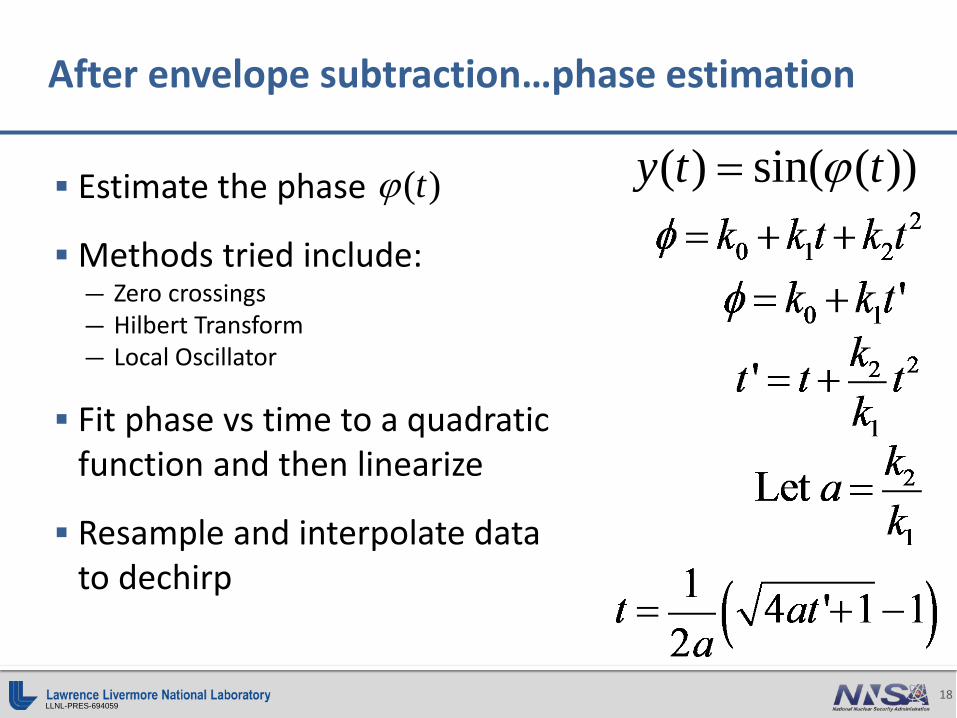
After envelope subtraction…phase estimation

Estimate the phase

Methods tried include:— Zero crossings— Hilbert Transform— Local Oscillator

Fit phase vs time to a quadratic function and then linearize

Resample and interpolate data to dechirp

))(sin()( tty ϕ=)(tϕ

LLNL-PRES-69405919

After dechirping

Envelope method: 200 point Loess smoothingPhase method: Zero crossings

LLNL-PRES-69405920

Before and after dechirping

LLNL-PRES-69405921

Distance to beat frequency calibration slope

Fit frequency to calibration distance to get the slope to use to correct future experimental data Conversion is .217 GHz/mm or 4.607 mm/GHz

56.3 mm is the “balance point” = no beat frequency

LLNL-PRES-69405922

Spectrogram of calibration measurements

LLNL-PRES-69405923

Another example: Sagebrush calibration measurements

Find envelope with Savitzky-Golay 220 point smoothing window

LLNL-PRES-69405924

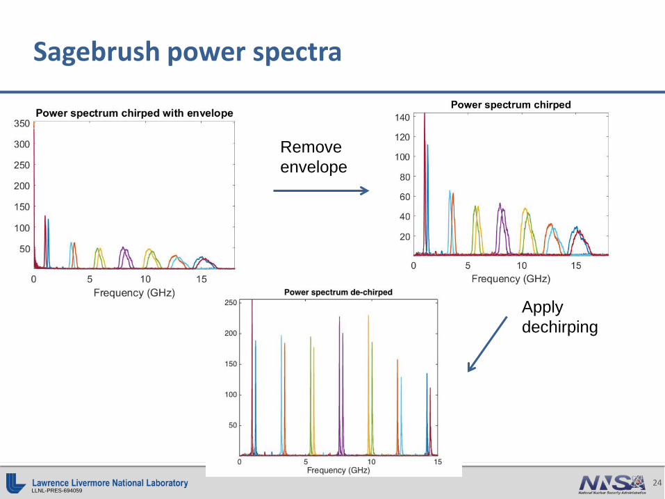
Sagebrush power spectra

Remove envelope

Apply dechirping

LLNL-PRES-69405925

Sagebrush: A closer look

LLNL-PRES-69405926

Sagebrush calibration analysis summary

Savitzky-Golay 220 points smoothing windowZero crossing phase estimationConversion: 2.271 mm/GHz

LLNL-PRES-69405927

A look at real data: explosive-driven aluminum test

Results show 12 cm target tracking with 14 GHz detection bandwidth