optical moorings-of-opportunity for validation of ocean color satellites

691

Journal of Oceanography, Vol. 64, pp. 691 to 703, 2008

Keywords:⋅⋅⋅⋅⋅ Optics,⋅⋅⋅⋅⋅ moorings,⋅⋅⋅⋅⋅ validation.

* Corresponding author. E-mail: [email protected]

Copyright©The Oceanographic Society of Japan/TERRAPUB/Springer

Optical Moorings-of-Opportunity for Validation of OceanColor Satellites

VICTOR S. KUWAHARA1*, GRACE CHANG2, XIAOBING ZHENG3, TOMMY D. DICKEY2

and SONGNIAN JIANG2

1Faculty of Education, Soka University, Tokyo 192-8577, Japan2Ocean Physics Laboratory, University of California Santa Barbara, 6487 Calle Real Suite A, Goleta, CA 93117, U.S.A.3Remote Sensing Department, Anhui Institute of Optics and Fine Mechanics, Hefei, China

(Received 24 September 2007; in revised form 3 April 2008; accepted 3 April 2008)

Buoy-mooring platforms are advantageous for time-series validation and vicariouscalibration of ocean color satellites because of their high temporal resolution andability to perform under adverse weather conditions. Bio-optical data collected onthe Bermuda Testbed Mooring (BTM) were used for comparison with satellite oceancolor data in an effort to further standardize sampling and data processing methodsfor high quality satellite-mooring comparisons. Average percentage differences be-tween satellite-measured and mooring-derived water leaving radiances were about20% at the blue wavelengths, decreasing to as low as 11% in the blue-green to greenwavebands. Based on a series of data processing methods and analyses, recommenda-tions concerning rigor of quality control for collected data, optimal averaging of high-frequency data, sensor self-shading wind corrections, and instrumentation placementrequirements are given for the design and application of optical moorings for oceancolor satellite validation. Although buoy-mooring platforms are considered to beamong the very best methods to validate ocean color satellite measurements, match-up discrepancies due to water column variability and atmospheric corrections re-main important issues.

are still needed for many operational and application pur-poses. The optimal utilization of ocean color imagersmounted on satellite platforms is constrained by severalfactors, including the quality and interpretation of theradiometric data sets. Of utmost importance to data qual-ity are the accuracy of the corrections (including quanti-fication of the degradation of optical detectors and at-mospheric effects) and the efficacy of ocean color algo-rithms that are required to relate satellite ocean colormeasurements to in-water quantities (O’Reilly et al.,1998; Fargion and Mueller, 2000; Hooker and McClain,2000; Pinkerton et al., 2003; IOCCG, 2006). Thus, it iscritical that remote sensing platforms be complementedwith continuous in situ measurements to generate andrefine the necessary algorithm input parameters for bio-optical products (i.e. Dickey et al., 2006).

One of the most successful approaches to validatingand vicariously calibrating remotely sensed ocean colordata has been the use of in situ optical measurements, i.e.ship-based, moored buoys, drifters and profiling floats(Chavez et al., 1997; Fargion and Mueller, 2000; Hooker

1. IntroductionNo other type of observational platform has had a

greater impact on large-scale, synoptic measurements ofthe marine biological environment than ocean color sat-ellites. Results obtained from ocean color imaging satel-lites such as the Nimbus-7 Coastal Zone Color Scanner(CZCS), the Sea-viewing Wide Field-of-view Sensor(SeaWiFS), and the Moderate-Resolution ImagingSpectroradiometer (MODIS) have greatly expanded ourknowledge of global distributions of phytoplankton, oceanprimary productivity, and biogeochemical fluxes (e.g.,Aiken et al., 1992; Hooker et al., 1992; Behrenfeld andFalkowski, 1997; Campbell et al., 2002; Behrenfeld etal., 2005). However, determinations of water columnproperties from satellite platforms are complicated andmajor improvements and increased information content

692 V. S. Kuwahara et al.

and McClain, 2000; Dickey et al., 2001, 2006; Struttonet al., 2001; Clark et al., 2003; Dickey, 2003; Kuwaharaet al., 2003; Pinkerton et al., 2003). In particular, theEulerian buoy-mooring observational platform has provento be an effective vehicle for both validation and vicari-ous calibration of ocean color satellites. Buoy-mooringplatforms are capable of sampling under even the mostadverse of weather and sea-state conditions with high tem-poral resolution for months at a time before the opticalsensors and system require servicing (Clark et al., 1997;Dickey et al., 2001, 2006). On the other hand, ocean colorsatellites are effectively restricted during even the slight-est cloud coverage and wind generated white-cap condi-tions. Multi-year deployments with periodic recoveriesand re-deployments of buoy-mooring systems fitted withoptical instrumentation (hereafter referred to as opticalmoorings) have become possible and successful as a re-sult of technological advances in hardware, powersources, data storage, telemetry capabilities, and copperanti-fouling devices (Chavez et al., 2000; Manov et al.,2004).

Optical moorings have formed the foundation of sev-eral long-term ocean monitoring projects and validationand/or vicarious calibration efforts (Chavez et al., 1997;Clark et al., 1997, 2003; Ishizaka et al., 1997; Kishino etal., 1997; Dickey et al., 1998, 2001, 2006; Letelier et al.,2000; Barnes et al., 2001; Strutton et al., 2001; Pinkertonet al., 2003; Spada et al., 2007). Moorings-of-opportu-nity can provide comprehensive, interdisciplinary in situobservations complementing satellite remotely senseddata for deriving synergistic descriptions of oceano-graphic features and their evolution in space and time, aswell as providing optical validation and, potentially, vi-carious calibration data. Optical moorings have helpedfacilitate ocean color satellite validation efforts by pro-viding high frequency, ground-truth measurements in avariety of open ocean locations; they have already col-lectively influenced correction techniques and algorithmdevelopment.

Although the potential of optical moorings has beendemonstrated, intercomparisons between different meas-urement and methodological techniques have yet to bestandardized. For example, protocols to calculate relevantin situ water-leaving radiance, Lw(λ), and normalizedwater-leaving radiance, Lwn(λ), have been recommended,but detailed descriptions of instrumentation placement,sampling frequency, site-specific limitations, etc. have yetto be standardized and are thus inconsistent between stud-ies (Kuwahara et al., 2003). In order to assure that radio-metric and bio-optical data acquired from optical moor-ings meet standards of quality and accuracy, clear andwell-documented sampling and data processing methodsneed to be standardized.

The purpose of this study is to make recommenda-

tions for the design and application of optical moorings-of-opportunity for ocean color satellite ground-truthingpurposes on a global scale. Specifically, we: (1) demon-strate that moorings-of-opportunity are viable platformsfor ocean color satellite validation by comparing in situoptical mooring and satellite ocean color match-ups ofLw(λ), (2) discuss the quality control and data analysisprotocols necessary for quality measurements, and(3) examine different ways to optimally deploy instru-mentation to minimize errors.

2. Materials and ProceduresData relevant to this study were collected on the

BTM, which was designed and configured to provide highfrequency in situ measurements at a fixed location in deepwaters off Bermuda for oceanographic science (Dickeyet al., 2001). The BTM is located at roughly 31°N, 64°W,about 80 km southeast of Bermuda in waters of ~4567 mdepth. BTM instrumentation of primary interest to thepresent study includes a chlorophyll fluorometer at 35 mand radiometers for upwelling radiance and downwellingirradiance. Each of the latter systems, co-located at 14and 21 m depths, utilize Satlantic, Inc. OCI-200 and OCR-200 radiometers that measure downwelling irradiance,Ed(λ, z), and nadir upwelling radiance, Lu(λ, z), at sevenwavelengths centered at 412, 443, 490, 510, 555, 665,and 683 nm (spectral bandwidth is 10 nm). These wave-lengths are compatible with those of the SeaWiFS oceancolor imager plus 683 nm. In addition to the subsurfaceradiometer packages, an OCI-200 was mounted on theBTM surface buoy just above the sea surface forEd(λ, 0+) and a Satlantic, Inc. Stordat-7 radiometer wasdeployed at 5 m depth to measure Lu(λ, 5m) at the sameseven wavelengths as those listed above. Sampling by theOCI/OCR-200 radiometers was done for 45 seconds at 6Hz every hour. The sampling rate for the Stordat-7 was 2Hz every hour for 30 seconds. All sensors were factorycalibrated following the standards set down by the oceancolor community (Mueller and Austin, 2003). Althoughpre- and post-calibrations of all radiometers were con-ducted, we utilized the post-calibration for the presentstudy since calibration drift was minimal for all instru-ments at all wavelengths (<1.5%). The data presented herewere collected during the 12th deployment of the BTM,between 30 July and 5 November 1999.

2.1 Data quality assurance/quality control (QA/QC)A data pre-processing routine was developed to se-

lect BTM data deemed appropriate for analysis. This rou-tine involved calculation of the calibrated measurementsfor the entire deployment at each wavelength for eachinstrument at each depth and a series of quality assur-ance and quality control (QA/QC) analyses, describedhere (Fig. 1A).

Ocean Color Validation Using Moorings 693

(1) The time-series data were inspected and scruti-nized for obvious data dropouts from instrument/powerfailure and symptoms of salt or other depositions on theoptical windows of the radiometers. Subsurface radiomet-ric data were subjected to the test for fouling followingwork by Abbott and Letelier (1998), who suggested thatdata are affected by bio-fouling when the upwelling radi-ance ratio of 683/555 nm exceeds 0.1, which is a valueappropriate for clear oligotrophic water masses such asthose found near Bermuda. In the present study, ratio val-ues for each depth (5, 15, and 21 m) were well below the0.1 threshold level, suggesting negligible influence frombio-fouling and effectiveness of precautionary anti-foul-ing methods (i.e. copper shutters; Manov et al., 2004).No data points showed signs of obvious instrument deg-radation or failure.

(2) The time-series of normalized spectra and wave-length-to-wavelength ratios from each surface and sub-surface data set were analyzed to determine the consist-ency and shape of each spectrum. The purpose of thisexercise is to determine whether the wavelength-to-wave-length ratio maintains consistency or “rank-order”throughout the deployment as defined by the relativemagnitude of normalized irradiance at all wavelengths,and to determine whether the wavelength-to-wavelengthratio values fall within limits defined by clear-sky mod-els of incident daylight (Kuwahara et al., 2003). It is ex-pected that the collected data should maintain a consist-ent normalized rank-order unless the instrument sensor

is damaged or improperly calibrated. The results obtainedfrom the time series of interest indicate that consistentwavelength-to-wavelength order was maintained; thisimplies that sensor diode integrity and reliable pre- andpost-deployment calibration prevailed.

(3) For incident spectral irradiance above the seasurface, Ed(λ, 0+), a comparison of the magnitudes ofmeasured Ed(λ, 0+) with clear-sky model Ed(λ, clear-sky)estimates by Frouin et al. (1989) were calculated for thesolar zenith angle at each measurement time for the en-tire deployment. Data were labeled as suspect if the inci-dent measurements exceeded a threshold factor of 1.25 ×Ed(λ, clear-sky). The factor 1.25 allows measured spec-tral irradiances to moderately exceed calculated clear-skyirradiances due to scattering from clouds. None of thedaily average Ed(λ, 0+) values failed this clear-sky qual-ity control test.

(4) Self-shading by the radiometers was correctedfollowing the methods presented by Gordon and Ding(1992). The error associated with radiometer self-shad-ing, ε(λ), can be represented as:

ε(λ) = [LuT(λ) – Lu

M(λ)]/LuT(λ), (1)

and

ε(λ) = 1 – exp[–k at(λ)r], (2)

where LuT(λ) is radiance corrected for self-shading and

Fig. 1. Flow-chart showing the procedures used during this study: data quality assurance/quality control (QA/QC), post-process-ing, and error analyses.


LuM(λ) is uncorrected radiance, at(λ) is the total absorp-

tion coefficient, r is the radius of the instrument housing(r = 0.44 m), and k = 2/tanθ0w (θ0w is the refracted solarzenith angle). This method assumes that absorption domi-nates over scattering processes, which is true for SargassoSea waters. The absorption coefficient was estimated us-ing the model presented by Morel (1991):

at(λ) = [aw(λ) + 0.06achl*(λ)Chl0.65][1 + 0.2y(λ)], (3a)

where

y(λ) = exp[–0.014(λ – 440)], (3b)

aw(λ) is the absorption coefficient of pure water (Popeand Fry, 1997), achl*(λ) is the chlorophyll-specific ab-sorption coefficient (Prieur and Sathyendranath, 1981),and Chl is the BTM-measured chlorophyll-a concentra-tion. Because values of at(λ) are extremely low in theSargasso Sea, radiometer self-shading effects were small,with ε(λ) ≈ 1%. We assumed that buoy-shading effectswere negligible; radiometers were mounted well belowthe base of the buoy (z ≥ 5 m) and on an arm extendingaway from the centerline of the mooring. In addition, sat-ellite and mooring match-up times used in this study wereall within two hours of Bermuda local noon, reducing theeffects of the buoy shading.

2.2 Data post-processingAfter performing the QA/QC protocols for moored

radiometric data, SeaWiFS and mooring data match-uptimes were identified. Successful match-ups are mostdependent on clear sky conditions and equivalent spatialcoverage (i.e. mooring occurring in a pixel). Of the en-tire 101-day BTM radiometric time series between 30 Julyand 5 November 1999, 23 suitable SeaWiFS satellitematch-ups were available, or roughly 23% of collecteddata. For comparison, PlyMBODy optical data, collectedin a relatively cloudy oceanic region (English Channel),matched up less than 6% of the time during a ~10 monthdeployment and about 10% of MOBY data are realizedfor SeaWiFS match-ups (Pinkerton et al., 2003). Thesedifferences underscore both the limitations and benefitsof using optical moorings-of-opportunity for satellite vali-dation and vicarious calibration, as moorings provideautonomously collected, long, continuous time series fromwhich satellite match-up data may be selected.

For the purpose of ocean color satellite validation itis necessary to average individual high-frequency meas-urements. The averaging of high frequency data accountsfor fluctuations in the incident light field, such as thosecaused naturally by wave-focusing (e.g., Zaneveld et al.,2001; Zheng et al., 2002), and allows comparisons to bemade with satellites using a single, averaged measure-

ment for a particular satellite image. For the BTM datasets, three different averaging techniques were tested. Foreach wavelength at each depth: (1) daily averages werecalculated using high-frequency data from 0700 to 1900Atlantic Standard Time (AST), (2) averages were com-puted for daily noon between 1000 and 1400 AST, and(3) 1-hr averages were computed, centered around thetime nearest to the SeaWiFS satellite overpass times. Sat-ellite overpass times were all within 1-hr of mooring datacollection.

The vertical diffuse attenuation coefficients fordownwelling irradiance and upwelling radiance, Kd(λ, z)and KL(λ, z), respectively, were determined directly fromQA/QC’ed radiometric measurements. Givendownwelling irradiance measured by radiometers at twodifferent depths, the diffuse attenuation coefficient fordownwelling irradiance at the midpoint of the two depthsis given by:

K ,zd

dzlnE , z ,

,

d dλ λ

λλ

( ) = − ( )[ ] ( )

= −( )( ) ( )

4a

1

zln

E , z

E , z4bd 2

d 1∆

where depths z2 > z1. Kd(λ, 18m) was computed usingmeasured Ed(λ, z) at 15 and 21 m. Further QA/QC analy-ses are performed on calculated Kd(λ, z); Kd(λ, z) shouldbe greater than the absorption coefficient of pure waterat each wavelength (Pope and Fry, 1997). Throughout thetime series, Kd(λ, 18m) values for λ = 665 and 683 nmfailed the pure water absorption coefficient test, likelydue to the low signal-to-noise ratio for Ed(λ, z) at the redwavelengths. Similar to Kd(λ, z), given two underwaterupwelling radiance sensors, the vertical attenuation co-efficient for upwelling radiance at the center of that depthinterval is calculated by:

K ,zd

dzln , z ,

.

L u

u 2

u 1

L 5a

1

zln

L , z

L , z5b

λ λ

λλ

( ) = − ( )[ ] ( )

= −( )( ) ( )

∆

KL(λ , 10m) was computed from measurements ofLu(λ, 5m) and Lu(λ, 15m), whereas KL(λ, 18m) was ob-tained using Lu(λ, z) measurements at 15 and 21 m, andfinally KL(λ, 13m) was calculated from Lu(λ, 5m) andLu(λ, 21m).

Water leaving radiance, Lw(λ), was determined byextrapolating upwelling radiance measured at depth z tothe surface following:


Lu(λ,0−) extrapolated using: Lu(λ,0−) extrapolated using:

Kd(18m) Lu(5m) Kd(18m) Lu(15m) Kd(18m) Lu(21m) KL(10m) Lu(5m) KL(18m) Lu(15m) KL(13m) Lu(21m)

Kd(18m) Lu(5m) 6 . 7 % 15% −−−−3.3% −13% −−−−4.6%

−−−−6.3% 0 . 1 6 % 3 . 2 % −23% −−−− 0 .05%

−37% −32% 19% −51% 10%

Kd(18m) Lu(15m) −−−−6.7% 7 . 9 % −−−−10% −20% −11%6 . 3 % 6 . 5 % 9 . 5 % −16% 6 . 3 %

37% 5 . 7 % 55% −14% 47%

Kd(18m) Lu(21m) −15% −−−−7.9% −18% −28% −19%

−−−− 0 .16% −−−−6.5% 3 . 0 % −23% −−−− 0 .21%32% −−−−5.7% 50% −20% 41%

KL(10m) Lu(5m) 3 . 3 % 10% 18% −−−−9.8% −−−−1.2%

−−−−3.2% −−−−9.5% −−−−3.0% −26% −−−−3.2%

−19% −55% −50% −57% −−−−8.8%

KL(18m) Lu(15m) 13% 20% 28% 9 . 8 % 8 . 6 %23% 16% 23% 26% 22%

51% 14% 20% 57% 60%

KL(13m) Lu(21m) 4 . 6 % 11% 19% 1 . 2 % −−−−8.6%0 . 0 5 % −−−−6.3% 0 . 2 1 % 3 . 2 % −22%

−−−−10% −47% −41% 8 . 8 % −60%

Table 1. Comparisons of Lu(λ, 0–) calculated using Eq. (6a) and vertical diffuse attenuation coefficients for upwelling radianceand downwelling irradiance computed at and extrapolated from various depths. Each table cell shows results at three wave-lengths: 412, 490, and 555 nm, respectively computed using averages between 0700 and 1900 AST. Percentage differenceswere calculated using Eq. (7) and averaged over the time series. Differences of less than 10% are indicated in bold.

L L e 6au uK ,z zLλ λ λ, , z ,0− ( )( ) = ( ) ( )

and through the surface according to:

Lw(λ) = 0.543Lu(λ, 0–), (6b)

where only nadir-viewing geometry is considered (thesurface reflectance becomes independent of wind speed)and the constant value, 0.543, corresponds to the upwardtransmittance term (Austin, 1974). Lu(λ, 0–) and Lw(λ)were computed 12 different ways using Eqs. (6a) and (6b):(1)–(3) KL(λ, 10m) and Lu(λ, z), (4)–(6) KL(λ, 13m) andLu(λ, z), and (7)–(9) KL(λ, 18m) and Lu(λ, z), where z =5, 15, and 21 m; Kd(λ, 18m) was substituted for KL(λ, z)and (10) Lu(λ, 5m), (11) Lu(λ, 15m), and (12) Lu(λ, 21m).For this study we present Lw(λ) rather than normalizedwater-leaving radiance, Lwn(λ), in order to evaluate ef-fects of solar zenith angle variability.

2.3 SeaWiFS data processingSeaWiFS data were provided by the NASA SIMBIOS

(National Aeronautics and Space Administration SensorIntercomparison for Marine Biological and Interdiscipli-

nary Ocean Studies) project for a 5 × 5 pixel box (roughly25 sq. km) centered on the nominal BTM location. The5 × 5 pixel box was selected as opposed to a 1 × 1 pixelbox to maximize satellite mach-ups due to environmen-tal variability at the BTM site and to provide more robustdata. A total of 1,251 SeaWiFS files (global and site-spe-cific local area coverage) were processed; 246 of thesefiles passed to Level 2 SeaWiFS products and were con-sidered useable. After reducing data points to those thathad at least one valid pixel in the 5 × 5 box, 87 match-upsremained. Of these 87 total match-ups, 46 local area cov-erage data points remained once the redundant data fromglobal area coverage were removed. Twenty-three of thesedata points matched-up with the BTM data collectionperiod and were used for the comparative analysis withthe BTM radiometer data. Due to frequent failure of thepure water absorption coefficient test, the red wavelengthsof 665 and 683 nm were not used in the analyses pre-sented here.

3. Assessment and ResultsIn the present study, downwelling irradiance and

upwelling radiance were measured on a mooring at mul-tiple depths, allowing us to establish the requirements for


reliable measurements necessary for validation of oceancolor satellite data.

3.1 Vertical diffuse attenuation coefficients, Kd(λ, z) andKL(λ, z)The vertical diffuse attenuation coefficients for

upwelling radiance and downwelling irradiance, KL(λ, z)and Kd(λ, z), evaluated for multiple depths were used toextrapolate Lu(λ, 0–) (Fig. 3). Comparisons were madebetween derived values of Lu(λ, 0–) (Table 1) to deter-mine the optimal placement of radiometers for satellitevalidation purposes. Percentage differences were com-puted using the following equation:

%, ,

. , ,,diff

L L

L L

u u

u u

λλ λ

λ λ( ) = ×

( ) − ( )[ ]( ) − ( )[ ]

( )− −

− −100

0 0

0 5 0 071 2

1 2

where the subscripts 1 and 2 specify two different meth-ods of computing Lu(λ, 0–), e.g., 1: using KL(λ, 10m) andLu(λ, 5m) and 2: using Kd(λ, 18m) and Lu(λ, 5m). Notethat these comparisons involved mooring measurementsonly. In general, derivations of Lu(λ, 0–) using Kd(λ, 18m)

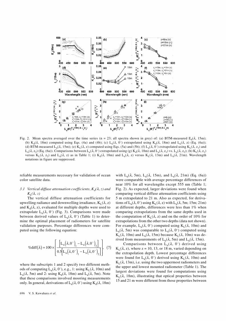
with Lu(λ, 5m), Lu(λ, 15m), and Lu(λ, 21m) (Eq. (6a))were comparable with average percentage differences ofnear 10% for all wavelengths except 555 nm (Table 1;Fig. 2). As expected, larger deviations were found whencomparing vertical diffuse attenuation coefficients using5 m extrapolated to 21 m. Also as expected, for deriva-tions of Lu(λ, 0–) using KL(λ, z) with Lu(λ, 5m; 15m; 21m)at different depths, differences were less than 1% whencomparing extrapolations from the same depths used inthe computation of KL(λ, z) and on the order of 10% forextrapolations from the other two depths (data not shown).For example, Lu(λ, 0–) computed using KL(λ, 10m) andLu(λ, 5m) was comparable to Lu(λ, 0–) computed usingKL(λ, 10m) and Lu(λ, 15m) because KL(λ, 10m) was de-rived from measurements of Lu(λ, 5m) and Lu(λ, 15m).

Comparisons between Lu(λ, 0–) derived usingKL(λ, z), where z = 10, 13, or 18 m, varied depending onthe extrapolation depth. Lowest percentage differenceswere found for Lu(λ, 0–) derived using KL(λ, 10m) andKL(λ, 13m), i.e. using the two uppermost radiometers andthe upper and lowest mounted radiometer (Table 1). Thelargest deviations were found for computations usingKL(λ, 18m), illustrating that optical properties between15 and 21 m were different from those properties between

Fig. 2. Mean spectra averaged over the time series (n = 23; all spectra shown in grey) of: (a) BTM-measured Ed(λ, 15m);(b) Kd(λ, 18m) computed using Eqs. (4a) and (4b); (c) Lu(λ, 0–) extrapolated using Kd(λ, 18m) and Lu(λ, z) (Eq. (6a));(d) BTM-measured Lu(λ, 15m); (e) KL(λ, z) computed using Eqs. (5a) and (5b); (f) Lu(λ, 0–) extrapolated using KL(λ, z1) andLu(λ, z2) (Eq. (6a)). Comparisons between Lu(λ, 0–) extrapolated using (g) Kd(λ, 18m) and Lu(λ, z1) vs. Lu(λ, z2); (h) KL(λ, z1)versus KL(λ, z2) and Lu(λ, z) as in Table 1; (i) Kd(λ, 18m) and Lu(λ, z) versus KL(λ, 13m) and Lu(λ, 21m). Wavelengthnotations in figure are suppressed.


SeaWiFS-measured: Lw(λ) derived using mooring:

Kd(18m) Lu(5m) Kd(18m) Lu(15m) Kd(18m) Lu(21m) KL(10m) Lu(5m) KL(18m) Lu(15m) KL(13m) Lu(21m)

Lw(412 nm) −56% −59% −62% −54% −49% −54%

−30% −37% −42% −25% −22% −25%

−23% −34% −40% −17% −17% −17%

Lw(443 nm) −60% −61% −65% −60% −50% −59%

−37% −41% −47% −35% −24% −34%

−32% −39% −45% −27% −20% −27%

Lw(490 nm) −57% −54% −57% −58% −46% −57%

−32% −31% −35% −32% −17% −30%

−26% −28% −34% −24% −12% −23%

Lw(510 nm) −64% −58% −52% −66% −45% −64%

−42% −36% −43% −45% −16% −42%

−38% −34% −41% −38% −11% −36%

Lw(555 nm) −61% −43% −47% −68% −34% −65%

−38% −13% −18% −47% 3.8% −42%

−33% −9.6% −16% −41% 11% −37%

Table 2. Comparisons between SeaWiFS-measured and mooring-derived values of Lw(λ). Each table cell shows three differentaveraging schemes: daily averaged (0700–1900 AST), 4-hr averaged (1000–1400 AST), and 1-hr averaged (nearest satelliteoverpass time) differences, respectively. Percentage differences were computed using Eq. (8) and averaged over the timeseries.

5 and 15 m. Lu(λ, 0–) derived using Kd(λ, z) versus thoseusing KL(λ, z) were comparable, except for KL(λ, 18m)(Table 1; Fig. 2). In general, differences computed at 555nm were greater than those at the other wavelengths. Ra-diance spectra were at a minimum at this wavelength; lowsignal-to-noise ratios in clear Sargasso Sea waters mayhave been the reason for poor correlations at 555 nm (Fig.2). Daily averaged (over daylight hours), 4-hr averaged(centered at noon), and 1-hr averaged (centered at over-pass) results were quite similar to each other.

BTM data showed that Kd(λ, z) was reliable in propa-gating Lu(λ, z) measurements at depth to just below thesurface. Because Kd(λ, z) undergoes a quality controlscreening (pure water absorption coefficient comparison)and it is an important variable in many bio-optical mod-els (e.g., Morel and Maritorena, 2001), it may be usefulin some operations to utilize Kd(λ, z) to extrapolateLu(λ, z) to the surface only, when KL(λ, z) is not readilyavailable. In other words, if a limited number of radiom-eters can be deployed or if some sensors fail, it may bedesirable to utilize one Lu(λ, z) sensor and two Ed(λ, z)sensors. Regardless of whether Kd(λ, z) or KL(λ, z) is (orboth are) used, sensors deployed at multiple depths arestrongly recommended to assure against data loss in theevent of sensor failure.

3.2 Water-leaving radianceWater-leaving radiances were computed using all

derived Lu(λ, 0–) quantities and Eq. (6b) (12 differentcomputations). These mooring-derived values were thencompared to SeaWiFS-measured Lw(λ) (Fig. 3; Table 2).Percentage differences were computed according to thefollowing equation:

%diff(λ) = 100 × [(Lw(λ)2 – Lw(λ)1)/Lw(λ)1], (8)

where Lw(λ)2 and Lw(λ)1 are water-leaving radiancesmeasured by SeaWiFS and derived from BTM radiomet-ric measurements, respectively. Comparisons betweensatellite-and mooring-derived Lw(λ) were wavelengthdependent. For the uppermost water column (5–15 m),percentage differences generally increased with wave-length. Interestingly, the opposite was true for Lw(λ) de-rived from Lu(λ, 21m). The reason for this is unknown.Pinkerton et al. (2003) reported higher absolute percent-age differences between SeaWiFS-measured andPlyMBODy-derived Lwn(λ) at the blue (412–443 nm) andred (670 nm) wavelengths (56 and 77%) compared to theblue-green to green wavebands (490–555 nm = ~20%),likely due to increased turbidity in the region.

BTM results showed that mooring data averaged over


daylight hours (0700–1900 AST) did not compare wellwith ocean color satellite measurements, which are col-lected at one instant in time. Absolute differences wereof the order of 50–70% for all wavelengths at all depthsusing KL(λ, z) or Kd(λ, 18m). On the other hand, resultsfor averaging performed over 4-hrs and 1-hr were im-proved as indicated by absolute differences of roughly25% (30–40%) and <20% (20–40%), respectively forLw(λ) derived using KL(412 nm, z) [Kd(412 nm, 18 m)](Fig. 3; Table 2). In all three time averaging cases, deri-vations using KL(λ, 18m) with Lu(λ, 15 and 21m) werebetter than those for KL(λ, 10m), KL(λ, 13m), orKd(λ, 18m). Recall that results from vertical diffuse at-tenuation coefficient comparisons showed that opticalproperties between 15 and 21 m were different from thoseproperties between 5 and 15 m.

4. DiscussionIn general, the differences between satellite-mea-

sured and BTM-derived Lw(λ) were comparable to thosefound using other optical moorings, except when aver-ages between 0700–1900 AST were used. Average dif-ferences over the SeaWiFS wavebands were 37% forPlyMBODy results (Pinkerton et al., 2003). Water-leav-ing radiance derived using KL(λ, 18m) and Lu(λ, 15m)were greatly improved, with differences of 20% in theblue, decreasing to 11% in the green wavebands. Variouserror analyses associated with in situ measurements were

conducted to evaluate the impact of: instrumentation in-accuracies (e.g., radiometric drift, miscalibrations,biofouling, wavelength shifts), mooring motion, and en-vironmental effects (solar angle and wind speed) on thediscrepancies related to methods of estimating Lw(λ) (Fig.1C). Radiance is an extremely difficult measurement tomake. For example, Chang et al. (2003) found differencesof ~20% between three different in situ methods of esti-mating Lw(λ).

4.1 Instrumentation effectsPropagation of errors from inaccurate measurements

of Ed(λ, z) and Lu(λ, z) caused by, e.g., radiometer drift,miscalibration, or biofouling, were investigated by com-puting Kd(λ, 18m) and KL(λ, 18m) from time-averagedBTM measurements of Ed(λ, z) and Lu(λ, z), where z =15 and 21, then varying these values of Kd(λ, 18m) andKL(λ, 18m) from 0 to ±100% by steps of ±20%. Water-leaving radiance was derived from variable values ofKd(λ , 18m) and KL(λ , 18m) and BTM-measured

Fig. 4. Kd(λ, 18m) and KL(λ, 18m) error analysis results.(a) Kd(λ, 18m) averaged over the time series (n = 23; blackline with closed circles) plotted with Kd(λ , 18m) ±Kd(λ, 18m) × 20%, 40%, 60%, 80%, and 100%. (b) As in(a) but for KL(λ, 18m). (c) and (d) Derived Lw(λ) using ver-tical diffuse attenuation coefficients in (a) and (b), respec-tively, and Eqs. (6a) and (6b). (e) and (f) Percent differ-ences in Lw(λ) (Eq. (8)).

Fig. 3. Time-averaged water-leaving radiance, Lw(λ), spectra(n = 23) measured by SeaWiFS and derived (a) usingKd(λ, 18m) and Lu(λ, z); (b) using KL(λ, z1) and Lu(λ, z2).Comparisons between Lw(λ) (c) derived using the three dif-ferent depths in (a); and (d) derived using the three differ-ent depth combinations in (b).


Lu(λ, 15m) (Eqs. (6a) and (6b)). The results of this analy-sis are shown in Fig. 4. Naturally, higher values of dif-fuse attenuation coefficients resulted in greater changes,therefore the computation of Lw(λ) using KL(λ, 18m) wasmuch more sensitive to changes than those usingKd(λ, 18m), and longer wavelengths were most affected.Moreover, increases as opposed to decreases inKd(λ, 18m) and KL(λ, 18m) resulted in higher percent-age differences between derived Lw(λ). Generally, a 20%error in the computation of Kd(λ, z) and KL(λ, z) resultedin <10% errors in the derivation of Lw(λ), however up to60% errors were found when KL(λ, z) was 100% of itstrue value (blue wavelengths). These errors increaseexponentially with increasing wavelength and would beeven greater for Case II water.

Variability in mooring-derived Lw(λ) can also be at-tributed to radiometer wavelength shifts (up to ±5 nmcaused by temperature variations). Wavelength shifts of+1 to +5 nm by steps of 1-nm were applied to measuredLu(λ, 5m) and Lu(λ, 15m). KL(λ, 10m) was then derivedfollowing Eqs. (5a) and (5b), and Lu(λ, 0–) and Lw(λ) werecomputed using Eqs. (6a) and (6b), extraolating fromLu(λ, 5m). Percentage differences were calculated usingEq. (8), with Lw(λ)2 = wavelength-shifted values andLw(λ)1 = non-wavelength-shifted values. Shifts of 1-nmresulted in <2.5% change across all wavelengths (aver-age difference was 1.3%), whereas ~6.5% changes oc-curred with a 5-nm shift (range of 2.2–13.2%). The blue-green wavelengths (490 and 510 nm) were most sensi-tive to wavelength shifts (data not shown). Results fromshifts of –1 to –5 nm were the same but of opposite sign.

4.2 Mooring motionVertical mooring heave effects on radiometric meas-

urements, which are dependent on weather and sea-stateconditions, were examined by deriving Lw(λ) fromLu(λ, 0–) extrapolated using a range of Kd(λ, z + ∆z) andKL(λ, z + ∆z) where z = 18 m for Kd(λ, z) and z = 5, 15,and 21 m for KL(λ, z), and ∆z was varied from 0.25 to 3m by steps of 0.25 m. Pressure sensors mounted on theBTM have measured the maximum heave of the BTM asabout 3 m. Percentage differences were computed usingEq. (8), where Lw(λ)2 = depth-shifted values and Lw(λ)1= non-depth-shifted values. The results show that heaveeffects increased with heave-depth (∆z) and depth of ver-tical attenuation coefficient, i.e. maximum effects wereseen for ∆z = 3 m and for derivations using KL(λ, 18m)(Fig. 5). Heave effects were also more prominent at 555nm than other wavelengths, although differences at 410nm for KL(λ, 10m) were relatively high. An upward moor-ing heave of 1-m resulted in differences between depth-shifted and non-depth shifted derivations of Lw(490 nm)ranging between 2.2% (3.4% for 555 nm) for KL(490 nm,10 m) to 3.2% (7.5% for 555 nm) for KL(490 nm, 18 m).Differences of 6.4% (9.8% for 555 nm) and 9.2% (20.9%for 555 nm) were found for Lw(490 nm) with a heave of3-m (Fig. 5). Heave effects can be corrected by using pres-sure sensors mounted at the same depth as radiometers.

Mooring horizontal motions related to the watch-cir-cle (i.e. maximum distance a mooring travels around itsanchor) have not been analyzed here, but horizontal vari-ability can affect satellite-to-mooring match-ups (Changand Gould, 2006). Mooring watch-circles are dependent

Fig. 5. Results from mooring heave error analysis. Lw(λ) spectra extrapolated using averaged (n = 23) (a) Kd(λ, 18m + ∆z) andLu(λ, 5m + ∆z); (b) KL(λ, 10m + ∆z) and Lu(λ, 5m + ∆z); (c) KL(λ, 13m + ∆z) and Lu(λ, 21m + ∆z); and (d) KL(λ, 18m + ∆z)and Lu(λ, 15m), and ∆z = 0.25 to 3 m by increments of 0.25 m. Percentage differences in Lw(λ) between non-depth-shifted(∆z = 0 m) and depth-shifted parameters (Eq. (8)) (e)–(h) derived using (a)–(d).


on water depth, wind speed and direction, currents, sea-state, and type of mooring design (i.e. semi-taught ver-sus catenary). The BTM watch-circle for the semi-taughtdesign is 5 km diameter whereas SeaWiFS and (MODIS-aqua) spatial resolution is ~1 km. Therefore, equivalentspatial coverage of SeaWiFS and mooring data may notbe obtained when matching the latitude and longitude ofthe mooring’s anchor with a satellite pixel. This does notpose a serious problem under horizontally homogeneousatmospheric and oceanic conditions, but may greatly af-fect match-ups in spatially variable environments (i.e.coastal ocean as described by Chang and Gould, 2006).Latitude and longitude obtained from a surface-mountedglobal positioning system (GPS) can help alleviate issuesassociated with mooring horizontal motions.

4.3 Environmental variabilityMismatches between satellite-measured and moor-

ing-derived Lw(λ) can also be attributed to environmen-tal conditions such as solar angle variability due to mis-matched satellite overpass times and variable wind speeds,which are related to transmission across the air-sea inter-face (Eq. (6b)). These factors were evaluated using theradiative transfer model, Hydrolight. Briefly, the well-documented Hydrolight model solves radiative transferequations in water, based on invariant imbedding theory(Mobley, 1994). Hydrolight output data relevant to this

study include Kd(λ, z), KL(λ, z) at z = 10, 13, and 18 m,and Lw(λ). Necessary inputs to Hydrolight include theboundary conditions and the inherent optical properties(IOPs). The IOPs were obtained from a historical Case Iwater model, assuming two components: pure water andchlorophyll-bearing particles with co-varying coloreddissolved organic matter and detritus. Pure water coeffi-cients were taken from Pope and Fry (1997). Chlorophyllconcentration (Chl) was assumed to be constant withdepth; Chl = 0.515 µg l–1, which was the average Chlmeasured by the BTM over the period of interest.Hydrolight input boundary conditions include wind speed,solar angle, cloud cover, downwelling sky irradiance, andocean bottom type. Cloud cover was held at 0%,downwelling sky irradiance was computed directly fromthe RADTRAN model and waters were assumed to beoptically deep (i.e. no influences from the ocean bottom).Two different simulations were run with these inputs:

(1) Wind speed was held constant at 5 m s–1 whilesolar angle was varied from 38.0 to 25.7°. The angles wereobtained by calculation of solar zenith angle between 1000and 1200 AST by steps of 15-min. In addition to the sam-pling time of day, these computations required latitudeand Julian day (JD; equations (2-2) and (2-3) from Kirk,1994). The latitude of the BTM is 31.7311°N and JD wasset at the approximate midpoint of the time series of in-terest, JD = 250 (7 September 1999). Differences were

Fig. 6. Results from environmental variability analysis. Simulated Lw(λ), Kd(λ, 18m) and KL(λ, 13m) computed using inputvariables described in Discussion: Environmental variability section and: (a)–(c) Variable solar zenith angles for 1000 to1200 AST, by increments of 15-min (symbols denote every 30-min) and (d)–(f) variable wind speeds.


evaluated between each solar angle and 25.7° (noontimesolar zenith angle), e.g., 25.7 compared to 38.0°, 25.7 and35.5°, etc. Solar angle had a great impact on computa-tions of Lw(λ), as indicated above. A 2-hr (1-hr) differ-ence in time resulted in ~15% (~4%) differences in de-rived Lw(λ). Lower wavelengths were slightly more af-fected by increasing solar angles (Fig. 6). Values ofKd(λ, z) and KL(λ, z) remained relatively unchanged (dif-ferences of <1%) until solar angle increased to more than7.5° from solar noon or >1.5 hours from 1200 AST. Dif-ferences then increased to 5–6%. These errors associatedwith solar zenith angle variability have been reduced sig-nificantly with the computation of Lwn(λ).

(2) Wind speed was varied from 0 to 15 m s–1 bysteps of 3 m s–1 while solar angle was held constant at30°. All other inputs were the same as for simulation (1).Differences reported were calculated between 0 m s–1 andeach increment of increasing wind speed, e.g., 0 and 3m s–1, 0 and 9 m s–1, etc. It was found that wind effectswere minimal, with less than 3.5% difference betweenLw(λ) computed for 0 m s–1 and 15 m s–1 wind speeds.Effects decreased with increasing wavelengths (Fig. 6).The influence of wind speeds on Kd(λ, z) and KL(λ, z)were similarly small (<2.2%) but increased with increas-ing wavelength (Fig. 6).

5. Recommendations and ConclusionsOur recommendations for the use of moorings-of-

opportunity for ocean color satelli te validation(oligotrophic waters) are as follows:

• Comparisons between the pre- and post-radiom-eter calibrations are essential (Mueller and Austin, 2003).It was confirmed that stringent comparisons between thetwo are necessary to verify how radiometer diodes mightdrift during deployment.

• Proper anti-biofouling precautions and proce-dures are essential for successful data collection. In ad-dition to shutters, wipers and anti-fouling material, werecommend that time-series data should be inspected forpotential fouling signals.

• QA/QC methods, e.g., clear-sky model and pure-water comparisons, must be employed and their usabilityhas been confirmed.

• Although instrument self-shading effects arerelatively small in clear, oceanic waters, correction fac-tors are relatively simple to compute and should be usedas confirmed in the present study.

• One-hour averages of high resolution time se-ries measurements of Ed(λ, z) and Lu(λ, z) centered near-est to the satellite overpass time showed the best resultscompared to other time-averaging methods, but 4-hr av-erages around daily noon are also suitable. Averaginghelps alleviate problems associated with wave focusing,intermittent cloud cover and other environmental vari-

ability at site.• Extrapolations of Lu(λ, z) to Lw(λ) are more

accurate when KL(λ, z) is used, as confirmed in the presentstudy. However, Kd(λ, z) can be a reasonable alternativeextrapolation variable. Here it is important to clarify thatalthough Kd(λ, z) and KL(λ, z) are completely differentoptical properties, in some instances when instrumentsfail and/or only instrument deployments are possible analternative option may be utilized.

• Pressure sensors should be co-located with ra-diometers to enable corrections due to mooring heave andinstrumentation effects, i.e. radiometer wavelength shiftsmust be considered.

• A surface buoy-mounted GPS is necessary foraccurate mooring-to-satellite pixel match-ups in horizon-tally variable environments.

• Radiometers should be placed within one opti-cal depth of the sea surface, above the subsurface chloro-phyll maximum, but also at a depth below the influenceof buoy shadowing effects. Procedures to address poten-tial buoy shadow effects are necessary.

• At least two upwelling radiance and twodownwelling irradiance sensors, i.e. sensor redundancy,are recommended in the case of sensor failure.

While dedicated calibration buoys such as theMOBY, YBOM and BOUSSOLE systems contribute todirect satellite vicarious calibration efforts, we show thatmoorings-of-opportunity can be cost-effective methodsfor validating data collected by ocean color satellites whenusing careful quality control procedures. Time-averagedpercentage differences between SeaWiFS-measured andBTM mooring-derived Lw(λ) were about 20% at the bluewavelengths, decreasing to as low as 11% in the blue-green to green wavebands. These results, however, do notmeet satellite ocean color goals of estimating Lwn(λ) towithin 5%. Nonetheless, these relatively small differencesare quite remarkable given the extreme difficulties in ac-curately measuring Lw(λ) in situ and remotely.

Our study shows that existing and future buoy-moor-ing systems are and will be essential to ocean color valida-tion and vicarious calibration. However, buoy-mooringsystems alone are not the complete answer as they onlyprovide documentation of discrepancies, not solutions.Future observational platform systems must include, forexample, robust measurements relating to atmosphericoptical and environmental conditions. Optical data froma wide variety of oceanic environments and complemen-tary interdisciplinary data for comparative analyses areessential to continuing improvements to the quality ofsatellite ocean color data and associated algorithms forthe derivation of environmentally importantbiogeochemical parameters (IOCCG, 1998, 1999, 2000,2004, 2006).


AcknowledgementsThe Bermuda Testbed Mooring (BTM) during the

time period of interest (Deployment #12) was supportedby the NSF Ocean Technology and Interdisciplinary Co-ordination Program, NSF Chemical Oceanography Pro-gram, and NSF Biological Oceanography Program (TD:OCE-9627281, OCE-9730471, OCE-9819477), NASA(TD: NAS5-97127), the ONR Ocean Engineering andMarine Systems Program (DF: N00014-96-1-0028 andN00014-94-1-0346), and the University of California,Santa Barbara. Derek Manov and Frank Spada of OPLare thanked for providing expert engineering and techni-cal support of the BTM and its optical instruments usedfor this study. Special thanks are extended to John Kempfor his dedication to the BTM, and to the Captain andcrew of the R/Vs Weatherbird II and Atlantic Explorerfor their continuing assistance at sea.

ReferencesAbbott, M. R. and R. M. Letelier (1998): Decorrelation scales

of chlorophyll as observed from bio-optical drifters in theCalifornia Current. Deep-Sea Res. II, 45, 1639–1667.

Aiken, J., G. F. Moore and P. M. Holligan (1992): Remote sens-ing of oceanic biology in relation to global climate change.J. Phycol., 28, 579–590.

Austin, R. W. (1974): The remote sensing of spectral radiancefrom below the ocean surface. p. 317–344. In Optical As-pects of Oceanography, ed. by N. G. Jerlov and E. S.Nielson, Academic.

Barnes, R. A., R. E. Eplee, G. M. Schmidt, F. S. Patt and C. R.McClain (2001): The calibration of SeaWiFS, Part 1: directtechniques. Appl. Opt., 40, 6682–6700.

Behrenfeld, M. J. and P. G. Falkowski (1997): A consumer’sguide to phytoplankton primary productivity models.Limnol. Oceanogr., 42, 1479–1491.

Behrenfeld, M. J., E. Boss, D. A. Siegel and D. M. Shea (2005):Carbon-based ocean productivity and phytoplankton physi-ology from space. Global Biogeochem. Cycles, 19, GB1006,doi:10.1029/2004GB002299.

Campbell, J., D. Antoine, R. Amstrong, K. Arrigo, W. Balch,R. Barber, M. Behrenfeld, R. Bidigare, J. Bishop, M. Carr,W. Esaias, P. Falkowski, N. Hoepffner, R. Iverson, D. Kiefer,S. Lohrenz, J. Marra, A. Morel, J. Ryan, V. Vedemikov, K.Waters, C. Yentsch and J. Yoder (2002): Comparison of al-gorithms for estimating ocean primary production from sur-face chlorophyll, temperature, and irradiance. GlobalBiogeochem. Cycles, 16, 1–15.

Chang, G. C. and R. W. Gould, Jr. (2006): Comparisons of op-tical properties of the coastal ocean derived from satelliteocean color and in situ measurements. Opt. Exp., 14,10,149–10,163.

Chang, G. C., E. Boss, C. Mobley, T. D. Dickey and W. S. Pegau(2003): Toward closure of upwelling radiance in coastalwaters. Appl. Opt., 42, 1574–1582.

Chavez, F. P., J. T. Pennington, R. Herlien, H. Jannasch, G.Thurmond and G. E. Friederich (1997): Moorings and drift-ers for real-time interdisciplinary oceanography. J. Atmos.

Oceanic Technol., 14, 1199–1211.Chavez, F. P., P. D. Wright, R. Herlien, M. Kelley, F. Shane and

P. G. Strutton (2000): A device for protecting mooredspectroradiometers from biofouling. J. Atmos. OceanicTechnol., 17, 215–219.

Clark, D. K., H. R. Gordon, K. J. Voss, Y. Ge, W. Broenkowand C. Trees (1997): Validation of atmospheric correctionover the oceans. J. Geophys. Res., 102, 17,209–17,217.

Clark, D. K., M. A. Yarbrough, M. Feinholz, S. Flora, W.Broenkow, Y. S. Kim, B. C. Johnson, S. W. Brown, M. Yuenand J. L. Mueller (2003): MOBY, a radiometric buoy forperformance monitoring and vicarious calibration of satel-lite ocean color sensors: measurement and data analysisprotocols. In Ocean Optics Protocols for Satellite OceanColor Sensor Validation, Volume VI, ed. by J. L. Mueller,G. S. Fargion and C. R. McClain, NASA/TM-2003-211621,NASA Goddard Space Flight Center.

Dickey, T. D. (2003): Emerging ocean observations for inter-disciplinary data assimilation systems. J. Mar. Syst., 40–41, 5–48.

Dickey, T., D. Frye, H. Jannasch, E. Boyle, D. Manov, D.Sigurdson, J. McNeil, M. Stramska, A. Michaels, N.Nelson, D. Siegel, G. Chang, J. Wu and A. Knap (1998):Initial results from the Bermuda Testbed Mooring Program.Deep-Sea Res. I, 45, 771–794.

Dickey, T. D., S. Zedler, D. E. Frye, H. Jannasch, D. Manov, D.Sigurdson, J. D. McNeil, L. Dobeck, X. Yu, T. Gilboy, C.Bravo, S. C. Doney, D. A. Siegel and N. Nelson (2001):Physical and biogeochemical variability from hours to yearsat the Bermuda Testbed Mooring site: June 1994–March1998. Deep-Sea Res. II, 48, 2105–2131.

Dickey, T. D., G. C. Chang and M. R. Lewis (2006): Opticaloceanography: recent advances and future directions usingglobal remote sensing and in situ observations. Rev.Geophys., 44, RG1001, doi:10.1029/2003RG000148.

Fargion, G. S. and J. L. Mueller (2000): Ocean optics protocolsfor satellite ocean color sensor validation, rev. 2. In NASATechnical Memo, 2000-209966, NASA Goddard SpaceFlight Center.

Frouin, R., D. W. Lingner, C. Gautier, K. S. Baker and R. C.Smith (1989): A simple analytical formula to compute clearsky total and photosynthetically available solar irradianceat the ocean surface. J. Geophys. Res., 94, 9731–9742.

Gordon, H. R. and K. Ding (1992): Self-shading of in-wateroptical instruments. Limnol. Oceanogr., 37, 491–500.

Hooker, S. B. and C. R. McClain (2000): The calibration andvalidation of SeaWiFS data. Prog. Oceanogr., 45, 427–465.

Hooker, S. B., W. E. Esaias, G. C. Feldman, W. W. Gregg andC. R. Maclain (1992): SeaWiFS Technical Report Series,An Overview of SeaWiFS and Ocean Color. p. 24. In NASATechnical Memorandum, 104566, Vol. 1, NASA GoddardSpace Flight Center.

IOCCG Report Number 1 (1998): Minimum requirements foran operational ocean-colour sensor for the open ocean.p. 46. In International Ocean Colour Coordinating Group,ed. by A. Morel.

IOCCG Report Number 2 (1999): Status and plans for satelliteocean-colour missions: Considerations for complementarymissions. p. 43. In International Ocean Colour Coordinat-


ing Group, ed. by J. A. Yoder.IOCCG Report Number 3 (2000): Remote sensing of ocean

colour in coastal and other optically-complex waters. p. 140.In International Ocean Colour Coordinating Group, ed. byS. Sathyendranath.

IOCCG Report Number 4 (2004): Guide to the creation anduse of ocean-colour, Level-3, binned data products. p. 88.In International Ocean Colour Coordinating Group, ed. byD. Antoine.

IOCCG Report Number 5 (2006): Remote sensing of inherentoptical properties: Fundamentals, tests of algorithms, andapplications. p. 126. In International Ocean Colour Coor-dinating Group, ed. by Z.-P. Lee.

Ishizaka, J., I. Asanuma, N. Ebuchi, H. Fukushima, H.Kawamura, K. Kawasaki, M. Kishino, M. Kubota, H.Masuko, S. Matsumura, S. Saitoh, Y. Senga, M. Shimanuki,N. Tomii and M. Utashima (1997): Time series of physicaland biological parameters off Shimane, Japan, during fallof 1993: First observation by moored optical buoy systemfor ADEOS data verification. J. Oceanogr., 53, 245–258.

Kirk, J. T. O. (1994): Light and Photosynthesis in Aquatic Eco-systems. 2nd ed., Cambridge University.

Kishino, M., J. Ishizaka, S. Saitoh, Y. Senga and M. Utashima(1997): Verification plan of OCTS atmospheric correctionand phytoplankton pigment by moored optical buoy sys-tem. J. Geophys. Res., 102, 17,197–17,207.

Kuwahara, V. S., P. G. Strutton, T. D. Dickey, M. R. Abbott, R.M. Letelier, M. R. Lewis, S. McLean, F. P. Chavez, A. H.Barnard and J. R. Morris (2003): Radiometric and bio-opti-cal measurements from moored and drifting buoys: meas-urement and data analysis protocols. p. 35–79. In OceanOptics Protocols for Satellite Ocean Color Sensor Valida-tion, Revision 4, Vol. VI: Special Topics in Ocean OpticsProtocols and Appendices, ed. by J. L. Mueller, G. S.Fargion and C. R. McClain, NASA/TM-2003-21621, NASAGoddard Space Flight Center.

Letelier, R. M., D. M. Karl, M. R. Abbott, P. Flament, M.Freilich, R. Lukas and T. Strub (2000): Role of late wintermesoscale events in the biogeochemical variability of theupper water column of the North Pacific Subtropical Gyre.J. Geophys. Res., 105, 28,723–28,739.

Manov, D. V., G. C. Chang and T. D. Dickey (2004): Methodsfor reducing biofouling of moored optical sensors. J. Atmos.Oceanic Technol., 21, 957–967.

Mobley, C. D. (1994): Light and Water: Radiative Transfer inNatural Waters. Academic.

Morel, A. (1991): Light and marine photosynthesis: A spectralmodel with geochemical and climatological implications.Prog. Oceanogr., 26, 263–306.

Morel, A. and S. Maritorena (2001): Bio-optical properties ofoceanic waters: A reappraisal. J. Geophys. Res., 106, 7163–7180.

Mueller, J. L. and R. Austin (2003): Characterization Oceano-graphic and Atmospheric Radiometers. p. 17–33. In OceanOptics Protocols for Satellite Ocean Color Sensor Valida-tion, Revision 4, Vol. II: Instrument Specifications, Char-acterization and Calibration, ed. by J. L. Mueller, G. S.Fargion and C. R. McClain, NASA/TM-2003-21621, NASAGoddard Space Flight Center.

O’Reilly, J., S. Maritorena, B. G. Mitchell, D. Siegel, K. L.Carder, S. Garver, M. Kahru and C. McClain (1998): Oceancolor chlorophyll algorithms for SeaWiFS. J. Geophys. Res.,103, 24,937–24,953.

Pinkerton, M. H., S. J. Lavender and J. Aiken (2003): Valida-tion of SeaWiFS ocean color satellite data using mooreddatabuoy. J. Geophys. Res., 108, 3133, doi:10.1029/2002JC001337.

Pope, R. M. and E. S. Fry (1997): Absorption spectrum (380–700 nm) of pure water. II. Integrating cavity measurements.Appl. Opt., 36, 8710–8723.

Prieur, L. and S. Sathyendranath (1981): An optical classifica-tion of coastal and oceanic waters based on the specificspectral absorption curves of phytoplankton pigments, dis-solved organic matter, and other particulate materials.Limnol. Oceanogr., 26, 671–689.

Spada, F. W., D. V. Manov and G. Chang (2007): Interdiscipli-nary ocean sensor technology development. Sea Tech.,March, 31–35.

Strutton, P. G., J. P. Ryan and F. P. Chavez (2001): Enhancedchlorophyll associated with tropical instability waves in theequatorial Pacific. Geophys. Res. Lett., 28, 2005–2008.

Zaneveld, J. R. V., E. Boss and P. A. Hwang (2001): The influ-ence of coherent waves on the remotely sensed reflectance.Opt. Exp., 9, 260–266.

Zheng, X., T. Dickey and G. Chang (2002): Variability of thedownwelling diffuse attenuation coefficient with considera-tion of inelastic scattering. Appl. Opt., 41, 6477–6488.

optical moorings-of-opportunity for validation of ocean color satellites

Documents