optical interferometry in practice eurosummer school observation and data reduction with the very...

Optical interferometry in practice

EuroSummer School

Observation and data reduction with the Very Large Telescope Interferometer

Goutelas, FranceJune 4-16, 2006

C.A.Haniff

Astrophysics Group, Department of Physics,University of Cambridge, UK

6th June 2006

VLTI EuroSummer School 26th June 2006C.A.Haniff – Optical interferometry in practice

A reminder of where we areA reminder of where we are

• Telescopes sample the fields at r1 and r2.

• Optical train delivers the radiation to a laboratory.

• Delay lines assure that we measure when t1=t2.

• The instruments mix the beams and detect the fringes.


Review of basic approach and rationaleReview of basic approach and rationale

• We need to measure the visibility function on a range of different baselines, each sensitive to structure on an angular scale /B.

• Interferometry is often the only way to investigate these scales.


OutlineOutline

• What are the things that make interferometry less than straightforward in practice?

– Sampling of the (u, v) plane

– Beam relay

– Delay compensation

– Beam combination

– Spatial wavefront fluctuations

– Temporal wavefront fluctuations

– Sensitivity

– Calibration


OutlineOutline



– Beam relay





– Sensitivity

– Calibration


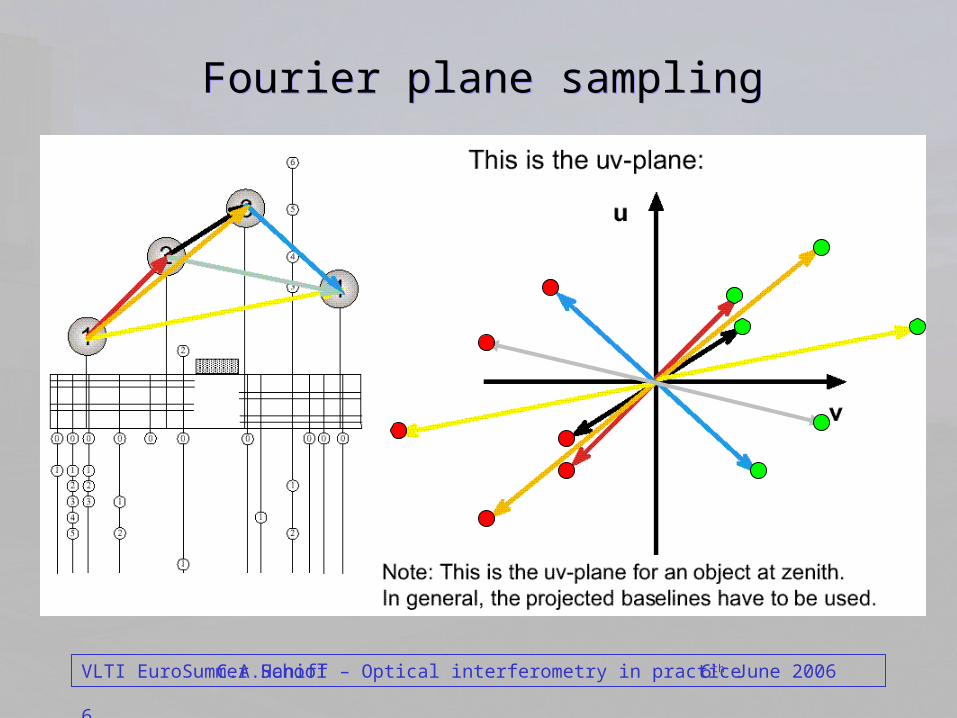
Fourier plane samplingFourier plane sampling


Fourier plane sampling (cont.)Fourier plane sampling (cont.)

• In practice rather than re-locate the telescopes to measure different spatial frequencies, we can often take advantage of the Earth’s rotation. In this case the tips of the uv vectors sweep out ellipses.

• The properties of these will be governed by:

– The hour angles of the observation.– The declination of the source.– The stations being used.

• Issues to be thinking about will include:

– Is there any shadowing of the telescopes by each other? – The allowed range of the delay lines - are they long enough?– The zenith distance - will the seeing be too poor at low elevations?

– Can the interferometer fringe-track ok?


Examples of Fourier plane coverageExamples of Fourier plane coverage

Whatever these look like, don’t forget the “rules of thumb”!

Dec -15 Dec -65


Image complexity and number of telescopesImage complexity and number of telescopes

4 telescopes, 6 hours

Model

8 telescopes, 6 hours


OutlineOutline



– Beam relay





– Sensitivity

– Calibration


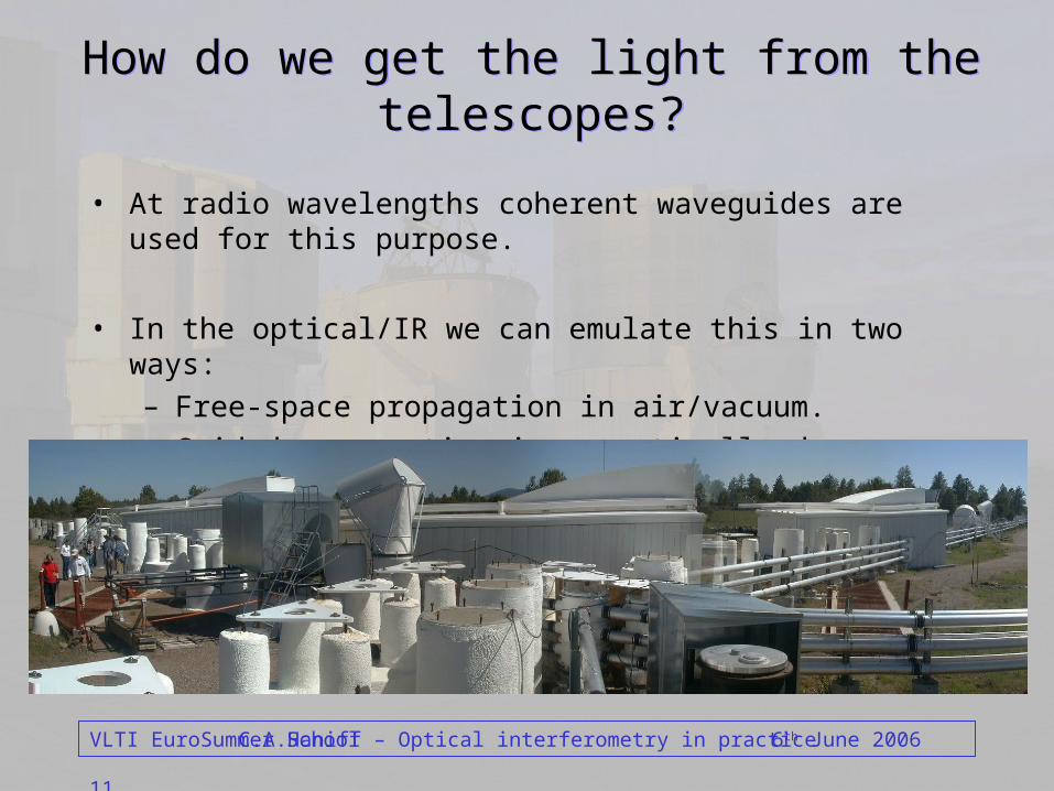
How do we get the light from the telescopes?How do we get the light from the telescopes?

• At radio wavelengths coherent waveguides are used for this purpose.

• In the optical/IR we can emulate this in two ways:

– Free-space propagation in air/vacuum.

– Guided propagation in an optically denser medium, e.g. using an optical fibre.


Issues for the beam relay implementationIssues for the beam relay implementation

• Whatever method is used, the following issues need to be managed:

– Longitudinal dispersion. i.e. the possibility of a mismatch in the optical paths in each interferometer arm due to the wavelength-dependence of the refractive index of the propagating medium.

– The polarization state of the propagating beams: this needs to be matched if the beams are to interfere successfully.

– How can a range of wavelengths be transported in parallel?

– How lossy is the propagation overall?

– How costly is the relay system?


Current preferencesCurrent preferences

• Currently, the most favoured approach has been to use free-space propagation in air-filled or evacuated pipes:

– Few problems existwith longitudinal dispersionand turbulence if the relaypipes are evacuated.

– For air-filled pipes a smallbeam diameter can help tolimit wavefront fluctuations.

– Generally a beam diameterD>(z)½ is used, where z is the propagation length, so as to mimimize diffraction losses.


• The key issues to take home are:

– Non-normal reflections will lead to differential amplitude and phase changes to be introduced into orthogonal polarization states. • As long as these are “identical” in each interferometer arm, the beams will

interfere.

– Polarizers placed either at the telescopes, or in front of the beam combiners, offer the possibility of disentangling the polarization and spatial structure of an arbitrary source.

An aside on polarizationAn aside on polarization

• In general there are two issues to deal with.

1. Can we control the polarization state sufficiently to interfere the beams from the telescopes?

2. Can we control the polarization state so as to make images of the sky in any polarization state we desire?

In most optical/IR implementations, problem (1) is always addressed, whereas problem (2) is generally left for “future generations” to think about!


OutlineOutline



– Beam relay





– Sensitivity

– Calibration


Why delay lines?Why delay lines?


Delay lines requirementsDelay lines requirements

• When the source is at the zenith no delay compensation is needed:

– VLTI has opdmax120m.

• The OPD correction varies roughly as B cos() d/dt, with the zenith angle.– VLTI has vmax 0.5cm/s

(though the carriages can move much faster than this).

• The correction has to be better than lcoh 2/.

– VLTI stability is 14nm rms.


Some practical caveatsSome practical caveats

• Unless very specialized beam-combining optics are used it is only possible to correct the OPD for a single direction in the sky.

– This is what gives rise to the FOV limitation: max [/B][/].

– This longitudinal dispersion implies that different locations of the delay line carts will be required to equalize the OPD at different wavelengths!

– For a 100m baseline and a source 50o from the zenith this OPD corresponds to 10m between 2.0-2.5m.

– More precisely, this implies the use of a spectral resolution, R > 5 (12) to ensure good fringe contrast (>90%) in the K (J) band.

• For an optical train in air, the OPD is actually different for different wavelengths since the refractive index n = n().


OutlineOutline



– Beam relay





– Sensitivity

– Calibration


Beam combinationBeam combination

• The essential principle here is:

Add the E fields, E1+E2, and then detect the time averaged intensity:

(E1+E2)(E1+E2)* = |E1|2 + |E2|2 + E1E2* + E2E1* = |E1|2 + |E2|2 + 2|E1||E2| cos() ,

where is the phase difference between E1 and E2.

• In practice there are two straightforward ways of doing this:

– Image plane combination:• AMBER and aperture masking experiments.

– Pupil plane combination:• MIDI and systems using fibre couplers (VINCI).


Image plane combinationImage plane combination• Mix the signals in a focal plane as in a Young’s slit experiment:

– In the focused image the transverseco-ordinate measures the delay.

– Fringes encoded by use of a non-redundant input pupil.

– The choice of the number of beamscombined is selected to optimise thesignal-to-noise.

– Possible to use dispersion prior todetection in the direction perpendicular to the fringesAllows measurement of the coherence function at multiple .


Pupil plane combinationPupil plane combination• Mix the signals by superposing afocal (collimated)

beams:

Then focus superposed beams ontoa single element detector.

– Fringes are visualised by measuring intensity versus time.

– Fringes encoded by use of a non-redundant modulation of delay ofeach beam.

– The number of beams combined isselected to optimise the S/N andspectral dispersion can be usedprior to detection.


Issues for the futureIssues for the future• Stability and throughput.

• Spectral bandpass.

• Ability to deal with large number of input beams.

Integrated optics 2 and 3-way combiners

Bulk optics 4-way 1-2.5m combiner.

10cm


OutlineOutline



– Beam relay





– Sensitivity

– Calibration


Spatial fluctuations of the wavefrontSpatial fluctuations of the wavefront


Spatial fluctuations of the wavefrontSpatial fluctuations of the wavefront

• These are characterized by Fried’s parameter, r0.

– The circular aperture size over which the mean square wavefront error is approximately 1 radian2.

– This scales as 6/5.

– The fluctuations exhibit a particularly steep spectrum: -11/3.

– And are potentially limited by an outer scale, L0, beyond which their strength saturates.

– Tel. Diameters > or < r0 delimit different regimes of instantaneous image structure:

• D < r0 quasi-diffraction limited images with image motion.

• D > r0 high contrast speckled (distorted) images.

– Median r0 value at Paranal is 15cm at 0.5m.


How do these spatial corrugations affect things?How do these spatial corrugations affect things?

A1 A3 A6 A10 AN, N>101.030 0.134 0.065 0.040 0.294 N -3/2

– Reduces the rms visibility (-----) amplitude as D/r0 increases.

– Leads to increased fluctuations in V.

– Both the above loss in sensitivity.

– Impacts on reliability of calibration.

– Moderate improvement is possiblewith tip-tilt correction ( ).

– Higher order corrections improvethings but more slowly.


SolutionsSolutions

• In principle, there are two approaches to deal with spatial fluctuations for telescopes of finite size:

/m 1.25 1.65 2.2 3.5 5.0ATs 3.8 2.7 1.9 1.1 0.7UTs 16.7 11.9 8.4 4.8 3.1

• Use an adaptive optics system correcting higher order Zernike modes:– Can use either the source or an off-axis reference star to sense atmosphere.– But need to worry about how bright and how far off axis is sensible.

• Instead, spatially filter the light arriving from the collectors:– Can use either a monomode optical fibre or a pinhole. – This trades off a fluctuating visibility for a variable throughput.


Spatial filteringSpatial filtering

Top secret


Getting the best of both worldsGetting the best of both worlds

• In fact, one can take advantage of both of these strategies:

– Solid = with spatial filter

– Dashed = without spatial filter.

– Different curves are for 2, 5 and 9 Zernike mode correction.

• Implications are:– For perfect wavefronts S/N D.– Spatial filtering always helps.

– Can work with large D/r0 (e.g. 10).

– If D/r0 is too large for the AO system, make D smaller.


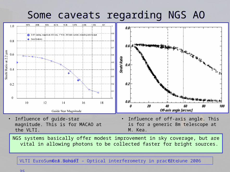
Some caveats regarding NGS AOSome caveats regarding NGS AO

• Influence of guide-star magnitude. This is for MACAO at the VLTI.

• Influence of off-axis angle. This is for a generic 8m telescope at M. Kea.

NGS systems basically offer modest improvement in sky coverage, but are vital in allowing photons to be collected faster for bright sources.


OutlineOutline



– Beam relay





– Sensitivity

– Calibration


The Earth’s atmosphere – temporal effectsThe Earth’s atmosphere – temporal effects


Temporal wavefront fluctuationsTemporal wavefront fluctuations• These are characterized by a coherence time, t0.

– Heuristically this is the time over which the wavefront phase changes by approximately 1 radian.

• Related to spatial scale of turbulence and windspeed:– Assume that Taylor’s “frozen turbulence” hypothesis holds, i.e.

that the timescale for evolution of the wavefronts is long compared with the time to blow past your telescope.

– Obtain a characteristic timescale t0 = 0.314 r0/v, with v a nominal wind velocity. Scales as 6/5.

• Typical values can range between 3-20ms at 0.5m.– Expect larger spatial scales to correspond to longer temporal ones.– Some evidence that windspeed is inversely correlated with r0.– Recent data from Paranal show median value of 20ms at 2.2m.


How does this temporal variation affect thingsHow does this temporal variation affect things• Temporal fluctuations provide a fundamental limit to the sensitivity of

optical arrays.

– Short-timescale fluctuations blur fringes:• Need to make measurements on

timescales shorter than ~t0.

– Long-timescale fluctuations move thefringe envelope out of measurableregion.

• Fringe envelope is few microns

• Path fluctuations tens of microns.

• Requires dynamic tracking of pistonerrors.


Perturbations to the amplitude and phase of VPerturbations to the amplitude and phase of V

• Apart from forcing any interferometric measurements to be made on a very short timescale, the other key problems introduced by temporal wavefront fluctuations are that they alter the phase of the measured visibility (i.e. coherence) function. Note that if the “exposure time is too long, they reduce the amplitude of the measured visibility too.

• How do we get around the problem of “altered” phases?

– Dynamically track the atmospheric excursions at the sub-wavelength level• Phase is then a useful quantity.

– Measure something useful that is independent of the fluctuations.• Relative phase.

• Closure phase.

Simple Fourier inversion of the coherence function becomes impossible.


Dynamic fringe tracking basicsDynamic fringe tracking basics

• We can identify several possible fringe-tracking systems:

– Those that ensure we are close to the coherence envelope.

– Those that ensure we remain within the coherence envelope.

– Those that lock onto the white-light fringe.

• The first two of these still need to be combined with short exposure times for any data taking.

• Only the last of these allows for direct Fourier inversion of the measured visibility function.

• As an aside, the second of these is generally referred to as “envelope” tracking or coherencing, while the third is often called “phase” tracking.


Envelope trackingEnvelope tracking

• Fringe envelope tracking methods - e.g. group delay tracking.

– Observe fringes in dispersed light.

– Dispersed fringes are tilted when OPD non-zero

– Recover fringe envelope position using 2-D power spectrum.

– Can integrate for several seconds – high sensitivity.

delay/

1/

FFT

FFT


Phase trackingPhase tracking

• The “easy” way:– Use a broad-band fringe tracking channel and lock onto white-

light fringe.

– Follow the fringe motion in real-time and sample fast enough so that fringe motion between samples is << 180 degrees.

– Can use a broad-band channel to phase-reference other narrow-band channels:

• Increases effective coherence time to seconds.

• Equivalent to self-referenced adaptive optics on the scale of the array.

– Because it’s a high precision technique it has 2.5 mag poorer sensitivity than group-delay tracking.


Off-axis phase referencingOff-axis phase referencing

– Use bright off-axis reference starto monitor the atmosphericperturbations in real-time.

– Feed corrections to parallel delay-lines observing science target.

– Use a metrology system to tie twooptical paths together.

• The “complex” way: dual-feed operation. This is what PRIMA aims to deliver:

In principle can extend effective coherence time by orders of magnitude if the white-light fringe is tracked.


Dual-feed interferometry (cont’d)Dual-feed interferometry (cont’d)

• Practical issues:

– Off-axis wavefront perturbationsbecome uncorrelated as field angleincreases and decreases.

– With 1 field-of-view <1% of skyhas a suitably bright reference source(H<12).

Off-axis reduction in mean visibility for the VLTI site as a function of D and .

– Metrology is non-trivial.

– Laser guide stars are not suitablereference sources.


Good observablesGood observables

• In the absence of a PRIMA-like system, optical/IR interferometrists have had to rely upon measuring phase-type quantities that are immune to atmospheric fluctuations.

• These are self-referenced methods - i.e. they use simultaneous measurements of the source itself:

– Reference the phase to that measured at a different wavelength - differential phase:

• Depends upon knowing the source structure at some wavelength.

• Need to know atmospheric path and dispersion.

– Reference the phase to those on different baselines - closure phase:• Independent of source morphology.

• Need to measure many baselines at once.


Closure phases (i)Closure phases (i)

• Measure visibility phase () on three baselines simultaneously.

• Each is perturbed from the true phase () in a particular manner:

12 = 12 + 1 - 2

23 = 23 + 2 - 3

31 = 31 + 3 - 1

• Construct the linear combination of these:

12+23+31 = 12 + 23 + 31

The error terms are antenna dependent

The source information is baseline dependent.


Closure phases (ii)Closure phases (ii)

• For an array of N telescopes, with N-1 unknown phase perturbations we can measure N(N-1)/2 visibility phases.

• This implies that there must be (N-1)(N-2)/2 quantities we can infer from our measurements that only depend on the source structure.

• The corresponding closure phases are one such set of these.

Ntels 3 4 5 8 NNbas 3 6 10 28 N(N-1)/2

Nclos_indep 1 3 6 21 (N-1)(N-2)/2Nclos_all 1 4 10 56 N(N-1)(N-2)/6

Frac_phase 0.33 0.50 0.60 0.75 1-(2/N)


Using “good” observablesUsing “good” observables

• Average them (properly) over many realizations of the atmosphere.

• Differential phase, if we are comparing with the phase at a wavelength at which the source is unresolved, is a direct proxy for the Fourier phase we need.

– Can then Fourier invert straightforwardly.

• Closure phase is a peculiar linear combination of the true Fourier phases:

– In fact, it is the argument of the product of the visibilities on the baselines in question, hence the name triple product (or bispectrum).

V12V23V31 = |V12| |V23| |V31| exp(I[12 + 23 + 31]) = T123

– So we have to use the closure phases as additional constraints in some nonlinear iterative inversion scheme.


OutlineOutline



– Beam relay





– Sensitivity

– Calibration


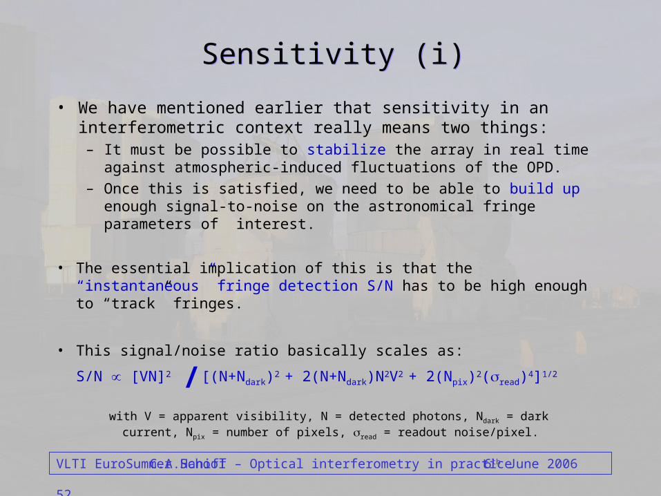
Sensitivity (i)Sensitivity (i)

• We have mentioned earlier that sensitivity in an interferometric context really means two things:– It must be possible to stabilize the array in real time against atmospheric-

induced fluctuations of the OPD.

– Once this is satisfied, we need to be able to build up enough signal-to-noise on the astronomical fringe parameters of interest.

• The essential implication of this is that the “instantaneous” fringe detection S/N has to be high enough to “track” fringes.

• This signal/noise ratio basically scales as:

S/N [VN]2 [(N+Ndark)2 + 2(N+Ndark)N2V2 + 2(Npix)2(read)4]1/2

with V = apparent visibility, N = detected photons, Ndark = dark current, Npix = number of pixels, read = readout noise/pixel.

/


Sensitivity (ii)Sensitivity (ii)

S/N [VN]2/[N2 + 2V2N3 +2Np24 ]1/2

[V2N] , with = 1/2 or 1.

• In general we want this to be > 1.

– Good fringe visibility is more important that more light.

– Resolved sources have V << 1. This implies very large reductions in the sensitivity of an interferometric array if the source being used to stabilize the array is resolved.

– On the longest interferometric baselines, the S/N will always be low.

– Don’t forget: bright sources are generally big - the small ones are faint!


Sensitivity (iii)Sensitivity (iii)

Apparent magnitudes of 1mas blackbodies of different temperatures.



Apparent magnitudes of 1mas blackbodies of different temperatures.



•This doesn’t mean that we shouldn’t improve the sensitivity of interferometers:

•All interesting sources aren’t blackbodies.

•Targets that are resolved need more flux to make a good measurement.

•But:

•Think about what is needed – always!


Sensitivity (iv)Sensitivity (iv)

• In summary:

– Need to have enough V2N to stabilize the array.

– Then we need to have enough integration time to build up a useful S/N on the science signal.

– The problem is that many sources of interest will have small V.

• Solutions:

– Use off-axis reference sources for stabilization (PRIMA).

– Decompose all long baselines into shorter ones where V is not so low.


OutlineOutline



– Beam relay





– Sensitivity

– Calibration


CalibrationCalibration

• The basic observables we wish to estimate are fringe amplitudes and phases.

• In practice the reliability of these measurements is generally limited by systematic errors, not the S/N we have just discussed.

• Hence there is a crucial need to calibrate the interferometric response:

– Measurements of sources with known amplitudes and phases:• Unresolved targets close in time and space to the source of interest.

– Careful design of instruments:• Spatial filtering.

– Measurement of quantities that are less easily modified by systematic errors:

• Phase-type quantities.


Examples of real dataExamples of real data

• Measurements with the NPOI

Perrin et al, AA, 331 (1998)

• Measurements with FLUOR

•


Examples of fake dataExamples of fake data

Preference fordefault model

Good reconstruction

“Poor” reconstruction

So you need to know what is required for the science.


SummarySummary• Sampling of the (u, v) plane

• What is needed for the scientific questions being addressed.• Will the array operate satisfactorily on these baselines.

• Beam relay• Maximum efficiency and stability.

• Delay lines• Intrinsic performance, dispersion at long baselines.

• Spatial fluctuations• Impact on sensitivity, potential limitations of AO.

• Temporal fluctuations• Impact on sensitivity, need for fringe tracking.• Good observables and how these are used.

• Sensitivity• An appropriate measure of this in terms of stabilizing the array.• V2N scaling.

• Calibration• Importance of matching this to the science desired.

optical interferometry in practice eurosummer school observation and data reduction with the very...

Documents

optical interferometry

hoursmodel8 telescopes

freespace propagation

guided propagation

optical train

optical paths

optical fibre

range of wavelengths