optical design with zemax - uni-jena.dedesign+wit… · illumination introduction in illumination,...
TRANSCRIPT

www.iap.uni-jena.de
Optical Design with Zemax
Lecture 9: Imaging
2013-01-08
Herbert Gross
Winter term 2012
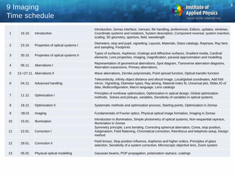
2 9 Imaging
Time schedule
1 16.10. Introduction
Introduction, Zemax interface, menues, file handling, preferences, Editors, updates, windows,
Coordinate systems and notations, System description, Component reversal, system insertion,
scaling, 3D geometry, aperture, field, wavelength
2 23.10. Properties of optical systems I Diameters, stop and pupil, vignetting, Layouts, Materials, Glass catalogs, Raytrace, Ray fans
and sampling, Footprints
3 30.10. Properties of optical systems II Types of surfaces, Aspheres, Gratings and diffractive surfaces, Gradient media, Cardinal
elements, Lens properties, Imaging, magnification, paraxial approximation and modelling
4 06.11. Aberrations I Representation of geometrical aberrations, Spot diagram, Transverse aberration diagrams,
Aberration expansions, Primary aberrations,
5 13.+27.11. Aberrations II Wave aberrations, Zernike polynomials, Point spread function, Optical transfer function
6 04.12. Advanced handling
Telecentricity, infinity object distance and afocal image, Local/global coordinates, Add fold
mirror, Vignetting, Diameter types, Ray aiming, Material index fit, Universal plot, Slider,IO of
data, Multiconfiguration, Macro language, Lens catalogs
7 11.12. Optimization I Principles of nonlinear optimization, Optimization in optical design, Global optimization
methods, Solves and pickups, variables, Sensitivity of variables in optical systems
8 18.12. Optimization II Systematic methods and optimization process, Starting points, Optimization in Zemax
9 08.01 Imaging Fundamentals of Fourier optics, Physical optical image formation, Imaging in Zemax
10 15.01. Illumination Introduction in illumination, Simple photometry of optical systems, Non-sequential raytrace,
Illumination in Zemax
11 22.01. Correction I
Symmetry principle, Lens bending, Correcting spherical aberration, Coma, stop position,
Astigmatism, Field flattening, Chromatical correction, Retrofocus and telephoto setup, Design
method
12 29.01. Correction II Field lenses, Stop position influence, Aspheres and higher orders, Principles of glass
selection, Sensitivity of a system correction, Microscopic objective lens, Zoom system
13 05.02. Physical optical modelling Gaussian beams, POP propagation, polarization raytrace, coatings
1. Fundamentals of Fourier optics
2. Physical optical image formation
3. Imaging in Zemax
3 9 Imaging
Contents
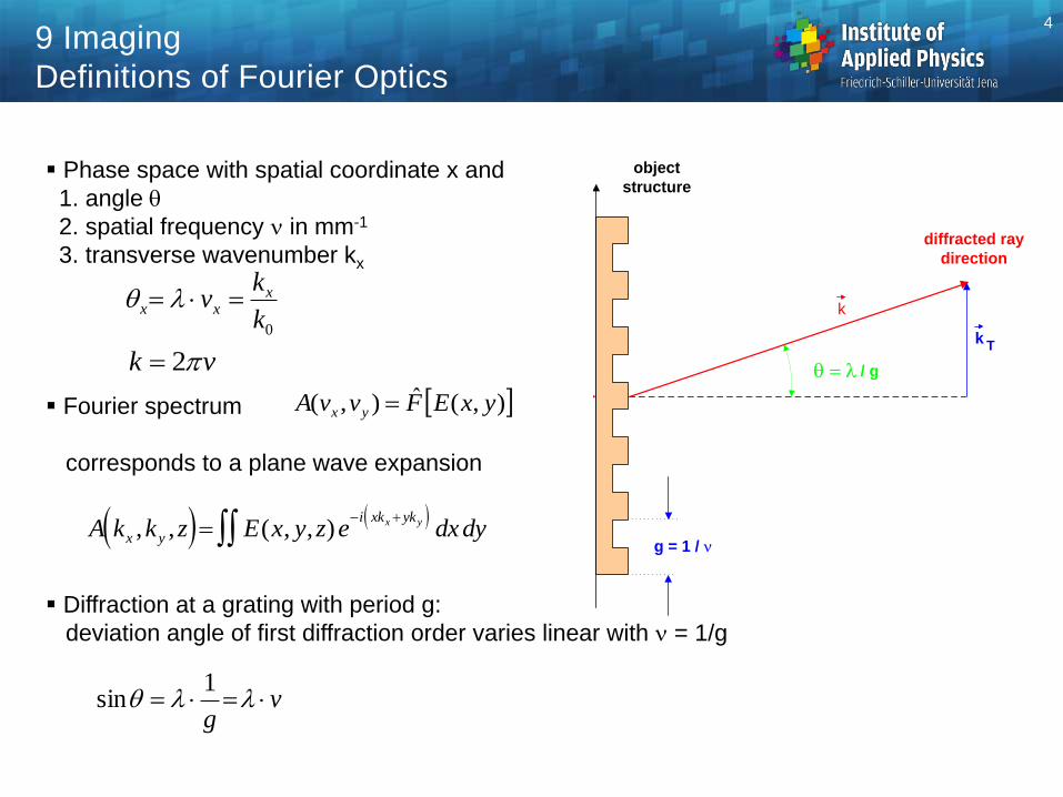
diffracted ray
direction
object
structure
g = 1 /
/ g
k
kT
9 Imaging
Definitions of Fourier Optics
Phase space with spatial coordinate x and
1. angle
2. spatial frequency in mm-1
3. transverse wavenumber kx
Fourier spectrum
corresponds to a plane wave expansion
Diffraction at a grating with period g:
deviation angle of first diffraction order varies linear with = 1/g
0k
kv x
xx
),(ˆ),( yxEFvvA yx
A k k z E x y z e dxdyx y
i xk ykx y, , ( , , )
vk 2
vg
1
sin
4
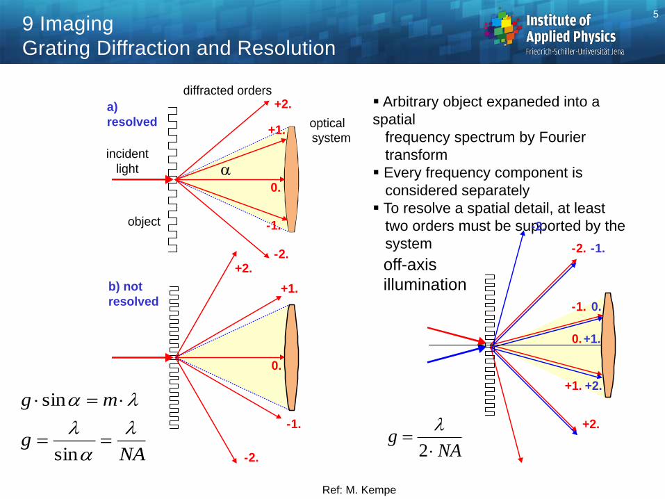
Arbitrary object expaneded into a
spatial
frequency spectrum by Fourier
transform
Every frequency component is
considered separately
To resolve a spatial detail, at least
two orders must be supported by the
system
NAg
mg
sin
sin
off-axis
illumination
NAg
2
Ref: M. Kempe
9 Imaging
Grating Diffraction and Resolution
optical
system
object
diffracted orders
a)
resolved
b) not
resolved
+1.
+1.
+2.
+2.
0.
-2.
-1.
0.
-2.
-1.
incident
light
+1.
0.
+2.
+1.
0.
+2.
-2.
-2. -1.
-1.
5
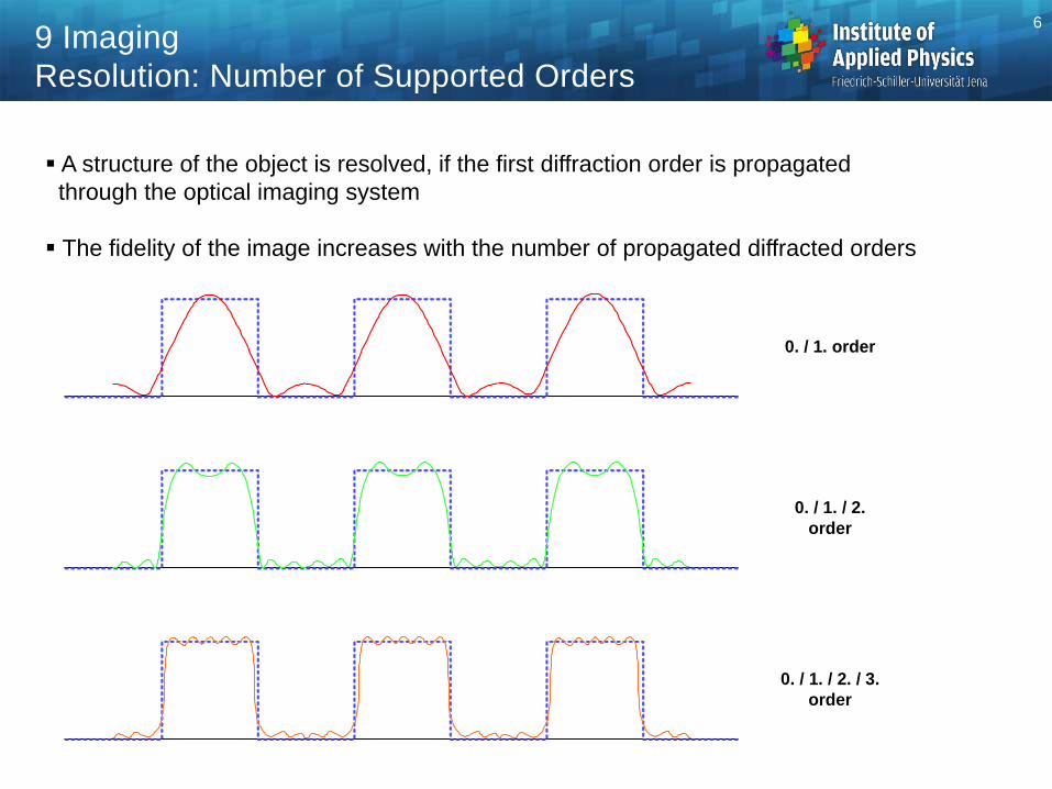
A structure of the object is resolved, if the first diffraction order is propagated
through the optical imaging system
The fidelity of the image increases with the number of propagated diffracted orders
0. / 1. order
0. / 1. / 2.
order
0. / 1. / 2. / 3.
order
9 Imaging
Resolution: Number of Supported Orders
6
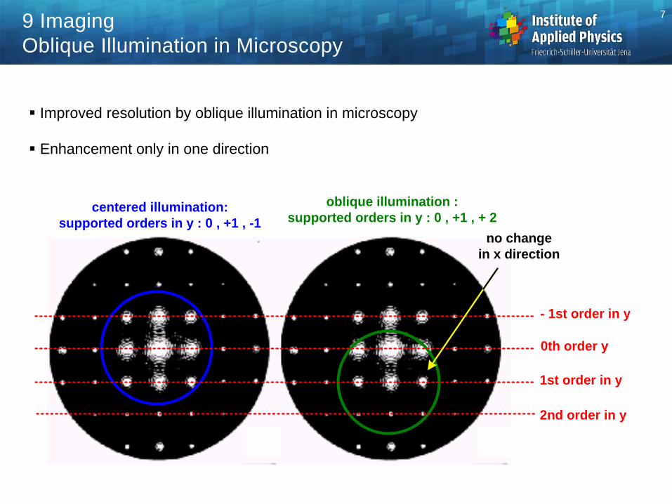
Improved resolution by oblique illumination in microscopy
Enhancement only in one direction
centered illumination:
supported orders in y : 0 , +1 , -1
oblique illumination :
supported orders in y : 0 , +1 , + 2
0th order y
1st order in y
2nd order in y
- 1st order in y
no change
in x direction
9 Imaging
Oblique Illumination in Microscopy
7

9 Imaging
Fourier Optical Fundamentals
Helmholtz wave equation:
Propagation with Green‘s function g,
Amplitude transfer function, impulse response
For shift-invariance:
convolution
Green‘s function of a spherical wave
Fresnel approximation
Calculation in frequency space: product
Optical systems:
Impulse response g(x,y) is coherent transfer function, point spread function (PSF).
G(x,y) corresponds to the complex pupil function
Fourier transform: corresponds to a plane wave expansion
),(*),','(),','( yxEzyyxxgzyxE
g r rr r
ei k r r
( , ' )'
'
1
4
g x y zi
ze eikz
i
zx y
( , , )( )
2 2
),(),,(),,( yxyxyx vvEzvvGzvE
)( 22
),,( yx vvziikz
yx ezvvG
dydxyxEyxyxgzyxE
),(),,','(),','(
8
9 Imaging
Diffraction at the System Aperture
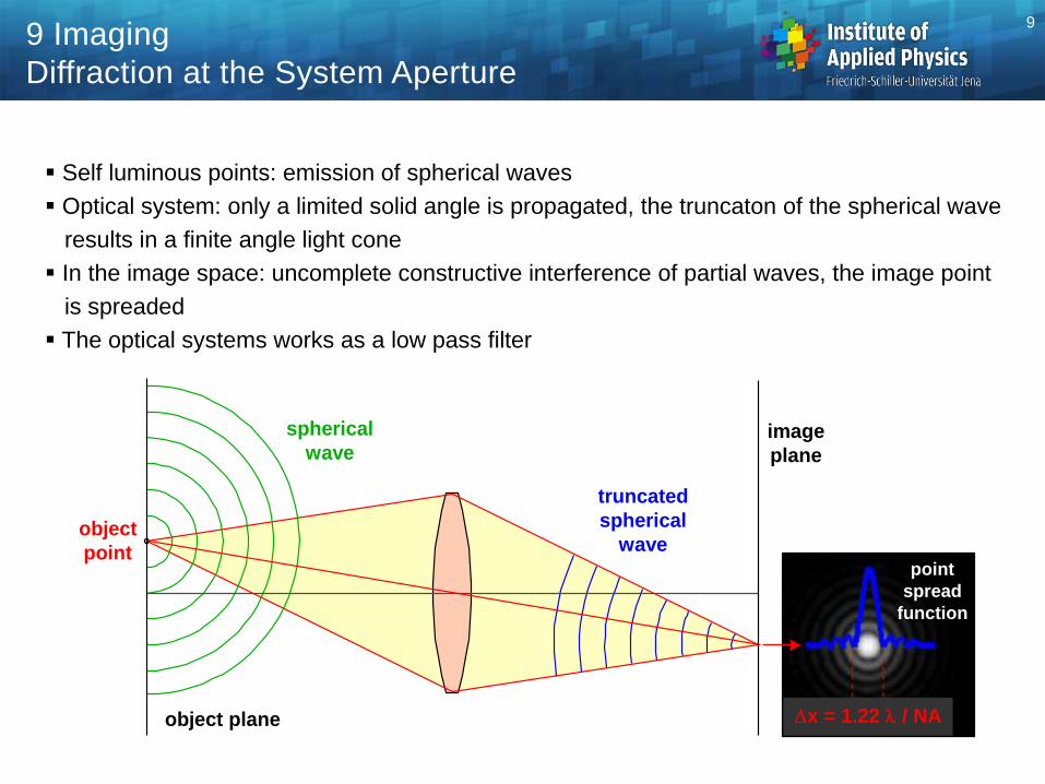
Self luminous points: emission of spherical waves
Optical system: only a limited solid angle is propagated, the truncaton of the spherical wave
results in a finite angle light cone
In the image space: uncomplete constructive interference of partial waves, the image point
is spreaded
The optical systems works as a low pass filter
object
point
spherical
wave
truncated
spherical
wave
image
plane
x = 1.22 / NA
point
spread
function
object plane
9

pppp
pp
vyvxi
pp
yxOTF
dydxyxg
dydxeyxg
vvH
ypxp
2
22
),(
),(
),(
),(ˆ),( yxIFvvH PSFyxOTF
pppp
pp
y
px
p
y
px
p
yxOTF
dydxyxP
dydxvf
yvf
xPvf
yvf
xP
vvH
2
*
),(
)2
,2
()2
,2
(
),(
9 Imaging
Optical Transfer Function: Definition
Normalized optical transfer function
(OTF) in frequency space
Fourier transform of the Psf-
intensity
OTF: Autocorrelation of shifted pupil function, Duffieux-integral
Absolute value of OTF: modulation transfer function (MTF)
MTF is numerically identical to contrast of the image of a sine grating at the
corresponding spatial frequency
10
x p
y p
area of
integration
shifted pupil
areas
f x
y f
p
q
x
y
x
y
L
L
x
y
o
o
x'
y'
p
p
light
source
condenser
conjugate to object pupil
object
objective
pupil
direct
light
at object diffracted
light in 1st order
9 Imaging
Interpretation of the Duffieux Iintegral
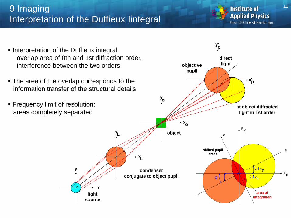
Interpretation of the Duffieux integral:
overlap area of 0th and 1st diffraction order,
interference between the two orders
The area of the overlap corresponds to the
information transfer of the structural details
Frequency limit of resolution:
areas completely separated
11
9 Imaging
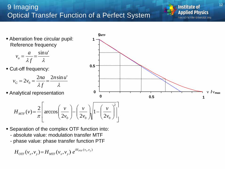
Optical Transfer Function of a Perfect System
Aberration free circular pupil:
Reference frequency
Cut-off frequency:
Analytical representation
Separation of the complex OTF function into:
- absolute value: modulation transfer MTF
- phase value: phase transfer function PTF
'sinu
f
avo
'sin222 0
un
f
navvG
2
000 21
22arccos
2)(
v
v
v
v
v
vvHMTF
),(),(),( yxPTF vvHi
yxMTFyxOTF evvHvvH
/ max
00
1
0.5 1
0.5
gMTF
12

I Imax V
0.010 0.990 0.980
0.020 0.980 0.961
0.050 0.950 0.905
0.100 0.900 0.818
0.111 0.889 0.800
0.150 0.850 0.739
0.200 0.800 0.667
0.300 0.700 0.538
9 Imaging
Contrast / Visibility
The MTF-value corresponds to the intensity contrast of an imaged sin grating
Visibility
The maximum value of the intensity
is not identical to the contrast value
since the minimal value is finite too
Concrete values:
minmax
minmax
II
IIV
I(x)
-2 -1.5 -1 -0.5 0 1 1.5 2
0
0.1
0.2
0.3
0.4
0.5
0.6
0.7
0.8
0.9
1
x
Imax
Imin
object
image
peak
decreased
slope
decreased
minima
increased
13
9 Imaging
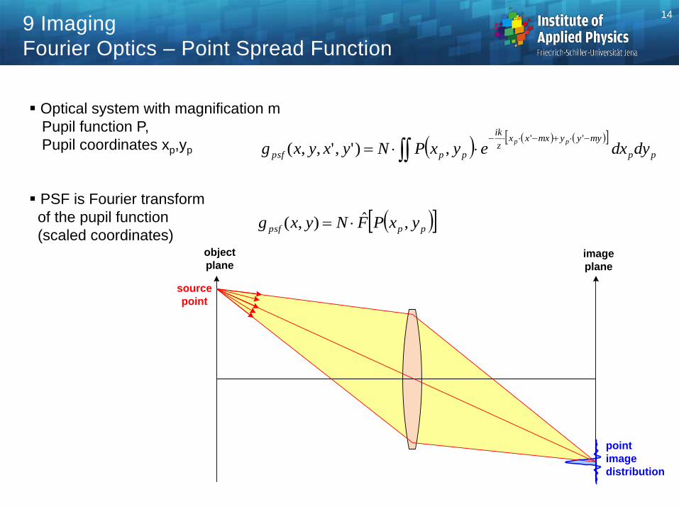
Fourier Optics – Point Spread Function
Optical system with magnification m
Pupil function P,
Pupil coordinates xp,yp
PSF is Fourier transform
of the pupil function
(scaled coordinates)
pp
myyymxxxz
ik
pppsf dydxeyxPNyxyxgpp ''
,)',',,(
pppsf yxPFNyxg ,ˆ),(
object
planeimage
plane
source
point
point
image
distribution
14
9 Imaging
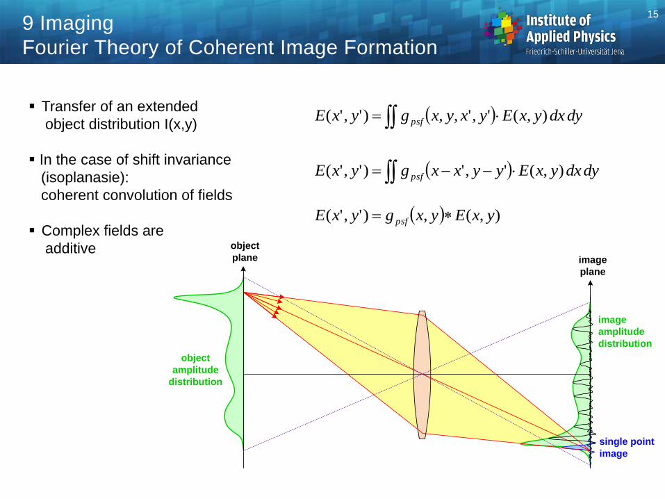
Fourier Theory of Coherent Image Formation
Transfer of an extended
object distribution I(x,y)
In the case of shift invariance
(isoplanasie):
coherent convolution of fields
Complex fields are
additive
object
plane image
plane
object
amplitude
distribution
single point
image
image
amplitude
distribution
dydxyxEyxyxgyxE psf ),(',',,)','(
dydxyxEyyxxgyxE psf ),(',')','(
),(,)','( yxEyxgyxE psf
15

9 Imaging
Fourier Theory of Coherent Image Formation
object
amplitude
U(x,y)
PSF
amplitude-
response
Hpsf (xp,yp)
image
amplitude
U'(x',y')
convolution
result
object
amplitude
spectrum
u(vx,vy)
coherent
transfer
function
hCTF (vx,vy)
image
amplitude
spectrum
u'(v'x,v'y)
product
result
Fourier
transform
Fourier
transform
Fourier
transform
16
9 Imaging
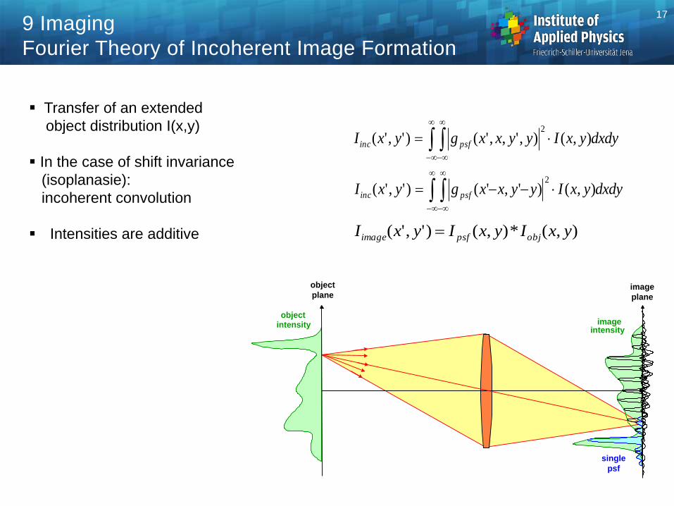
Fourier Theory of Incoherent Image Formation
objectintensity image
intensity
single
psf
object
planeimage
plane
Transfer of an extended
object distribution I(x,y)
In the case of shift invariance
(isoplanasie):
incoherent convolution
Intensities are additive
dydxyxIyyxxgyxI psfinc
),()','()','(2
),(*),()','( yxIyxIyxI objpsfimage
dydxyxIyyxxgyxI psfinc
),(),',,'()','(2
17
9 Imaging
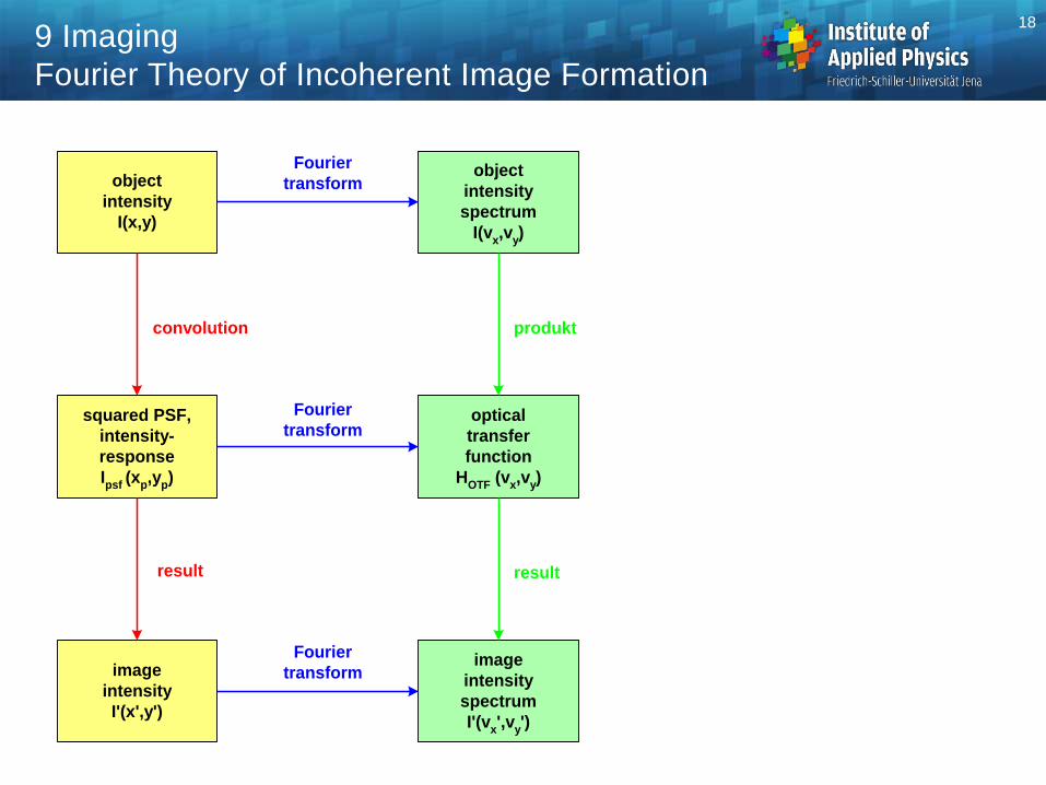
Fourier Theory of Incoherent Image Formation
object
intensity
I(x,y)
squared PSF,
intensity-
response
Ipsf
(xp,y
p)
image
intensity
I'(x',y')
convolution
result
object
intensity
spectrum
I(vx,v
y)
optical
transfer
function
HOTF
(vx,v
y)
image
intensity
spectrum
I'(vx',v
y')
produkt
result
Fourier
transform
Fourier
transform
Fourier
transform
18
9 Imaging
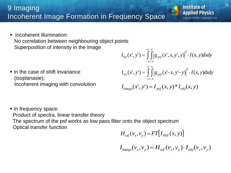
Incoherent Image Formation in Frequency Space
Incoherent illumination:
No correlation between neighbouring object points
Superposition of intensity in the image
In the case of shift invariance
(isoplanasie):
Incoherent imaging with convolution
In frequency space:
Product of spectra, linear transfer theory
The spectrum of the psf works as low pass filter onto the object spectrum
Optical transfer function
dydxyxIyyxxgyxI psfinc
),()','()','(2
),(*),()','( yxIyxIyxI objpsfimage
dydxyxIyyxxgyxI psfinc
),(),',,'()','(2
),(),( yxIFTvvH PSFyxotf
),(),(),( yxobjyxotfyximage vvIvvHvvI
19

Circular disc with diameter
D = d x Dairy
Small d << 1 : Airy disc
Increasing d:
Diffraction ripple disappear
0 0,5 1 1,5 210 -4
10 -3
10 -2
10 -1
10 0
d = 0.1
d = 0.2
d = 0.5
d = 1.0
d = 1.5
d = 2.0
Log I(r)
rsinu /
d = 0.1 d = 0.2 d = 0.5 d = 1.0 d = 1.5 d = 2.0
9 Imaging
Incoherent Image of a Circular Disc
20
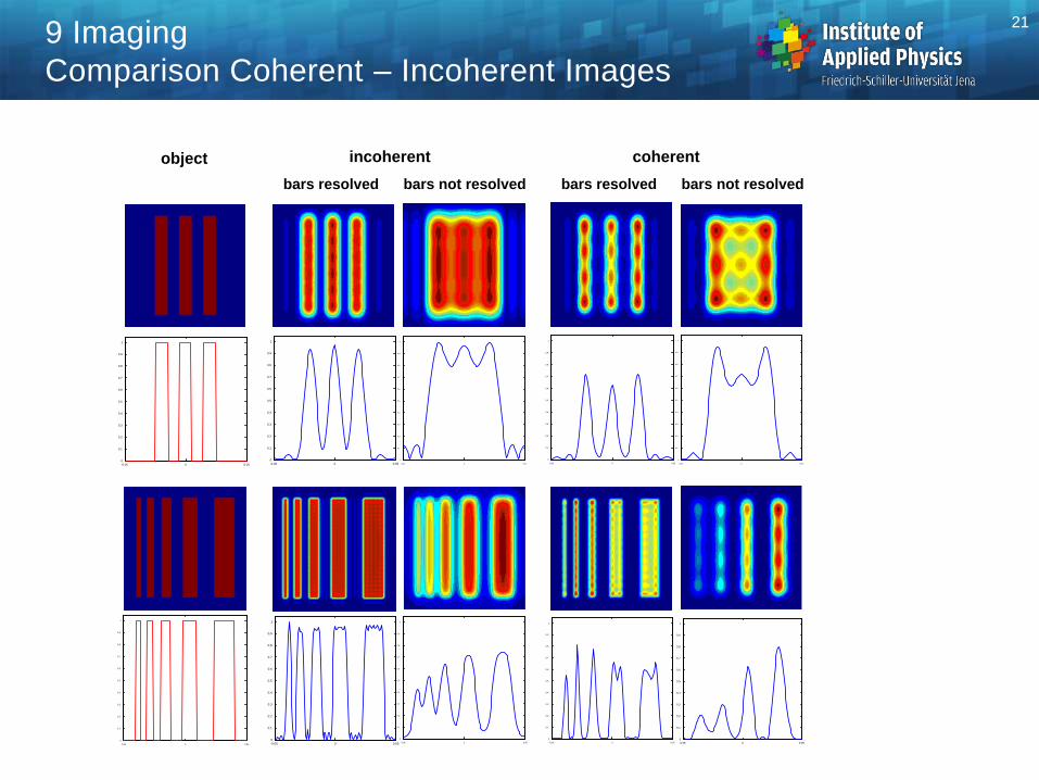
9 Imaging
Comparison Coherent – Incoherent Images
object
-0.05 0 0.05
0
0.1
0.2
0.3
0.4
0.5
0.6
0.7
0.8
0.9
1
incoherent coherent
-0.05 0 0.05
0
0.1
0.2
0.3
0.4
0.5
0.6
0.7
0.8
0.9
1
-0.05 0 0.05
0
0.1
0.2
0.3
0.4
0.5
0.6
0.7
0.8
0.9
1
-0.05 0 0.05
0
0.1
0.2
0.3
0.4
0.5
0.6
0.7
0.8
0.9
1
-0.05 0 0.05
0
0.1
0.2
0.3
0.4
0.5
0.6
0.7
0.8
0.9
1
-0.05 0 0.05
0
0.1
0.2
0.3
0.4
0.5
0.6
0.7
0.8
0.9
1
-0.05 0 0.05
0
0.1
0.2
0.3
0.4
0.5
0.6
0.7
0.8
0.9
1
-0.05 0 0.05
0
0.1
0.2
0.3
0.4
0.5
0.6
0.7
0.8
0.9
1
-0.05 0 0.05
0
0.1
0.2
0.3
0.4
0.5
0.6
0.7
0.8
0.9
1
-0.05 0 0.05
0
0.1
0.2
0.3
0.4
0.5
0.6
0.7
0.8
0.9
1
bars resolved bars not resolved bars resolved bars not resolved
21

Possible options in Zemax:
Convolution of image with Psf
1. geometrical
2. with diffraction
Geometrical raytrace analysis
1. simple geometrical shapes (IMA-files)
2. bitmaps
Diffraction imaging:
1. partial coherent
2. extended with variable PSF
Structure of options in Zemax not clear
Redundance
Field definition and size scaling not good
Numerical conditions and algorithms partially not stable
22 9 Imaging
Imaging in Zemax
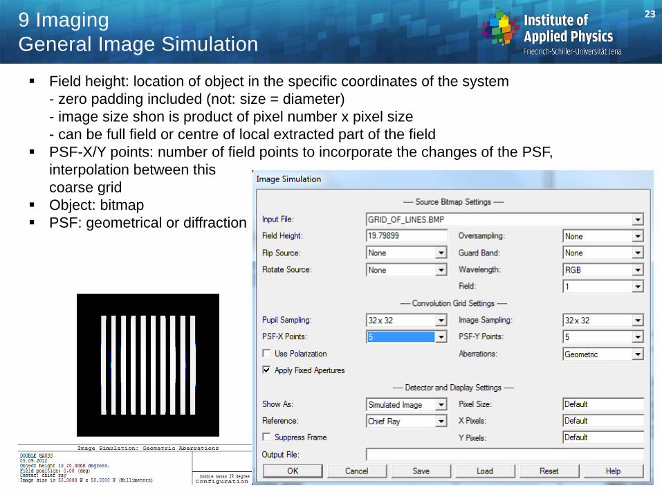
Field height: location of object in the specific coordinates of the system
- zero padding included (not: size = diameter)
- image size shon is product of pixel number x pixel size
- can be full field or centre of local extracted part of the field
PSF-X/Y points: number of field points to incorporate the changes of the PSF,
interpolation between this
coarse grid
Object: bitmap
PSF: geometrical or diffraction
23 9 Imaging
General Image Simulation

Total field size: defined by system
Field height/size: reduced field corresponding to the structure as considered in the
imaging calculation
Field position: reference point of the considered reduced field (center) in the total field
Image size: size of the represented field size, should be a little larger as field size
to clearly see the boundary
In some tools calculated as product of pixel number and pixel size
24 9 Imaging
General Image Simulation
total field of
the system
field height/
field size
image size /
pixel size times
pixel number
field
position /
field index
x
y

Geometrical imaging by raytrace
Binary IMA-files with geometrical shapes
Choice of:
- field size
- image size,
- wavelengths
- number of rays
Interpolation possible
25 9 Imaging
Geometric Imaging I
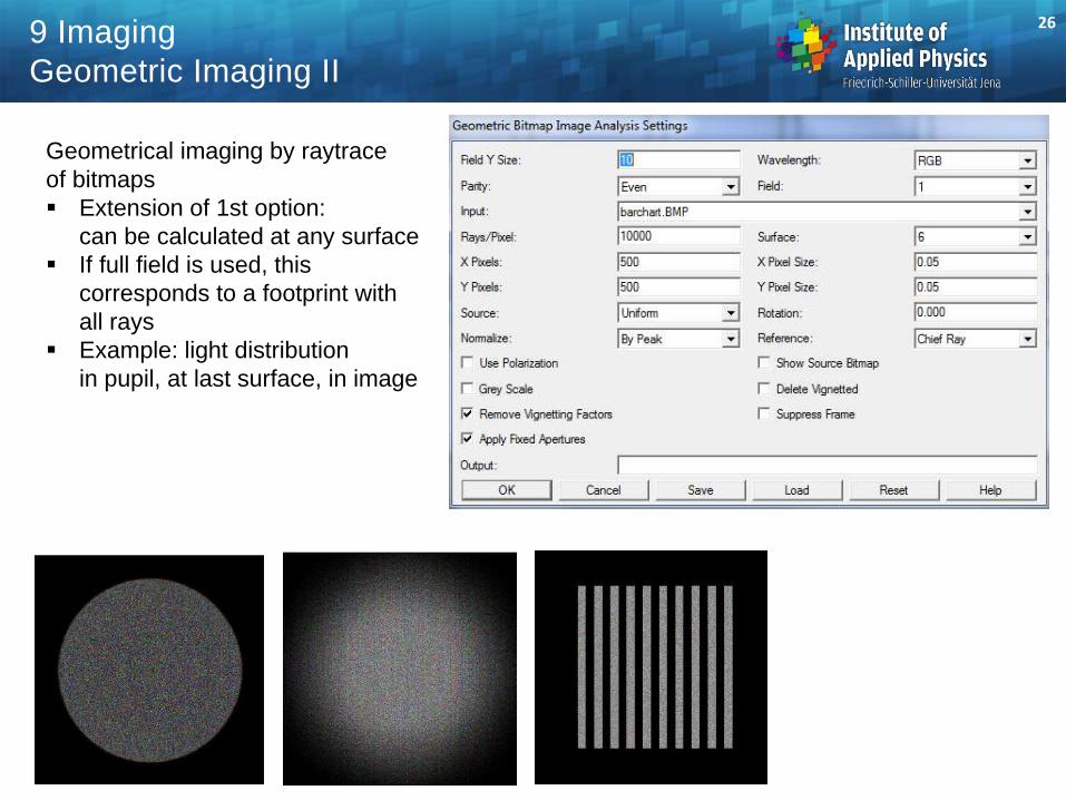
Geometrical imaging by raytrace
of bitmaps
Extension of 1st option:
can be calculated at any surface
If full field is used, this
corresponds to a footprint with
all rays
Example: light distribution
in pupil, at last surface, in image
26 9 Imaging
Geometric Imaging II

Different types of partial coherent model algorithms possible
Only IMA-Files can be used as objects
describes the coherence factor (relative pupil filling)
Control and algorithms not clear, not stable
27 9 Imaging
Patial Coherent Imaging

Classical convolution of psf
with pixels of IMA-File
Coherent and incoherent
model possible
PSF may vary over field
position
28 9 Imaging
Extended Diffraction