OPG/NSERC Research ChairWatershed Biochemistry

2001-2002 Workshop ReportMay 21-22, 2002

July 30, 2002

Summary of Contents

Peter Dillon Introduction to the workshop …………………………………………. 2

Julian AherneCritical loads of sulphur and nitrogen — steady-state water chemistry and first-order acidity balance models………………………………. 7

Shaun Watmough Acid deposition and the terrestrial environment…………………….. 9

Keith SomersPatterns in climate parameters.Understanding the role of climate signals……………………………. 11

Jim ButtleThresholds influencing slope – riparian zone – stream coupling:an example from the Canadian Shield……………………………….. 14

Catherine EimersSources and Controls of Sulphur Cycling in Muskoka-HaliburtonCatchments……………………………………………………………. 16

Peter DillonLake Mass Balances………………………………………………….. 18

Sherry SchiffDissolved Organic Matter, What can isotopes tell us?……………….. 20

Julian AherneMAGIC — simulating drought induced sulphate peaks in stream chemistry at Plastic Lake…………………………………. 21

Dean JeffriesRecovery of aquatic ecosystems in south eastern Canada from acidicdeposition…………………………………………………………….. 23

Bill KellerRecovery of Acidified Lakes near Sudbury, Ontario, Canada……….. 28

Norman YanBiological effects of acid deposition…………………………………. 31

Keith Somers, Bioassessments: The effects of stressors on streams.Why do (rapid) bioassessments?……………………………………………. 34

Julie Schulenburg Master Thesis Proposal: Determining the impacts of golf course construction and operation on the benthic macroinvertebrate communities in streams on the Precambrian Shield………………… 37

Isabelle LavoieDoctoral Thesis Proposal: Diatoms as a biological indicatorof water quality in streams of Ontario and Quebec………………….. 38

Andrew Paterson Paleolimnological Studies: Acid deposition/ Climate Change………. 39

Lewis MolotPhoto-Oxidation of Humic DOC in Northern Lakes…………………. 41

Dolly KothawalaMaster Thesis Project: Spatial and temporal patterns of dissolvedorganic carbon (DOC) molecular size distribution by high performance size exclusion chromatography (HPSEC)……………… 43

APPENDIX A. References…………………………………………….49

APPENDIX B. List of Addresses…………………………………….. 51

1

OPG/NSERC Research ChairWatershed Biochemistry

1) Introduction to workshop Peter Dillon2) Environmental Research Supported by OPG Greg Pope

Rob Lyng3) Critical loads of S and N – the SSWC and FAB models Julian Aherne4) Acid deposition and the terrestrial environment Shaun Watmough5) Patterns in climate parameters Keith Somers6) Hydrology, flowpaths, source areas Jim Buttle7) Controls on sulphur cycling in catchments Cathy Eimers8) Lake mass balances – S, N Peter Dillon9) Nitrogen cycling in catchments Sherry Schiff

10) MAGIC Julian Aherne11) Recovery from acid deposition in Canada Dean Jeffries12) Recovery in the Sudbury region Bill Keller13) Biological effects of acid deposition Norm Yan14) Bioassessment: the effects of stressors on streams Keith Somers15) Rapid bioassessment – benthos Julie Schulenburg16) Bioassessment using stream periphyton Isabelle Lavoie17) Paleolimnological studies: acid deposition, climate change Andrew Paterson18) Photochemistry of DOC Lew Molot19) DOC speciation Dolly Kothawalla

2

Peter Dillon, Introduction to the workshop

Dr. Peter Dillon opened the workshop and presented the background information that ledto the research chair and the partnership between Ontario Power Generation (OPG), NSERC andTrent University.

The scientific programme of the OPG/NSERC Industrial Research Chair in WatershedBiogeochemistry was designed in response to anticipated increases in sulphur (S) and nitrogen(N) emissions from Ontario Power Generation Inc. In 1996, fossil power accounted for just 13%of OPG’s total power production capacity, but increased to 27% by 1999. Although measuresbased on technological methods were employed by OPG to keep emission rates below the cap setby regulation, deposition of strong acid anions (sulphate and nitrate) was expected to rise inresponse to the increased emissions. As well, emissions and possibly deposition of trace metalssuch as mercury (Hg) were anticipated to increase.

In addition to changing acid deposition rates, there is strong evidence that climatepatterns in many parts of the world including Ontario are being altered very substantially as aresult of global increases in greenhouse gas concentrations, and that changes in stratosphericozone are influencing the level of ultraviolet radiation that is reaching the earth’s surface.Moreover, other stressors are affecting our environment on a large spatial scale. It is also evidentthat these stresses do not act independently, but interact in ways that accelerate ecosystemdegradation. As part of an industry that contributes to the Canadian pool of carbon emissions,OPG has an interest in the effects of climate change as well as an interest in acid deposition.

In Canada, nearly 45% of the land area is considered sensitive to acid deposition, andlakes and watersheds located on the Canadian Shield are considered the most vulnerable, due tothe low buffering capacity of the typically shallow soils that overlay Shield bedrock. A largeportion of eastern Canada, including much of Ontario and Quebec as well as the AtlanticProvinces is underlain by granitic bedrock of the Canadian Shield, and this area also receives thehighest levels of acid deposition in the country.

The Watershed Biogeochemistry research programme focuses on some of these sensitivelakes and their catchments in the Muskoka-Haliburton region of south-central Ontario, an areawhich receives currently approximately 50 meq/m2 of SO4 and 55 meq/m2 N (as NO3

-, NH4+)

annually, and which is almost entirely underlain by acid-sensitive soils. A number of catchmentsin this region have been studied since the early 1980s, and have shown negative chemical andbiological effects of acidification. In response to previous reductions in industrial S emissions,however, about half of the lakes studied in this region had shown signs of recovery (as indicatedby decreasing sulphate concentration), while the remaining half had shown no positive responseto changes in deposition. Furthermore, those that had shown some positive change had improvedmarkedly less than expected based on the change in deposition. It was apparent that the responseof lakes and their catchments to changes in acid deposition is variable, and is likely modified bywithin-catchment processes.

Projects planned as part of the research programme were intended to improve ourunderstanding of the way in which biogeochemical processes in lakes’ watersheds control their

3

rate of degradation when the deposition of strong acids increases and their rate of recovery whenacid deposition rates decline. Furthermore, because it was apparent that environmentalperturbations such as acid deposition do not act in isolation, but are often augmented or offset byother factors, the interaction between changes in climate and acid deposition was intended to be amajor focus of the research. The research programme was designed to consider the effects ofspecific climate perturbations such as summer droughts on the chemical and biological responseof aquatic ecosystems, and to differentiate between those effects mediated by changes in aciddeposition and those brought about by a varying climate.

Four projects were initiated to address these research objectives:

· Evaluation of existing environmental data in Ontario related to surface and groundwaterchemistry, to assess the likelihood that expected changes in acid deposition will result inmeasurable changes in water quality.

· Measurement of the chemical and biological response of aquatic ecosystems to changesin OPG’s sulphur emissions including: (i) measurement and modeling of the chemicalresponse of a representative set of lakes and their terrestrial catchments (ii) assessment ofbiological effects using simple indicators, and (iii) evaluation of the changes in mercurydeposition related to fossil fuel use.

· Evaluation of the interrelationships between climate change, the sulphur cycle in lakesand watersheds, and changes in emission and deposition of acid precursors, with specificreference to El Niño episodes.

· Investigation of the role of dissolved organic carbon (DOC) in integrating the effects ofmultiple stressors including acid deposition, changing climate and others.

Project 1 Analysis of Long-term Trends

1A Changes in Long-term ChemistryActivities:· Analysis of long-term chemical data sets at Dorset (32 lakes, 24 streams)· Comparison with trends/patterns in Norway, at Turkey Lakes, ELA, Wisconsin· Collaboration with EU project, RECOVER 2010 on recovery rates and

controlling factors

H0 (1): Spatial pattern of recovery in lakes is a function of catchment physiography, i.e.wetland area.H0 (2): Temporal pattern of recovery in lakes is a function of climate, specifically the ElNino pattern.

4

Collaborators:Bob Ferrier (Macaulay Land Use Research Institute, UK)Dean Jeffries (Environment Canada)Alan Jenkins (Centre for Ecology and Hydrology, UK)Kathy Webster (U. Wisconsin, USA)Richard Wright (NIVA, Norway)

1B PaleolimnologyActivities:· Collection of sediment cores available from lakes with long-term chemical

records for analysis of acid deposition and climate effects· Tree core collection from gauged catchment(s) for analysis of deposition and

climate effects

H0 (1): Temporal pattern over the long-term and climate variables, particularly El Nino,are coherent.H0 (2): There has been a decrease in some ions/metals (Ca) and an increase in others (Al)available to forests in acidified catchments.

Collaborators:Brian Cumming (Queens U.)Roland Hall (U. Waterloo)Andrew Paterson (Queens U.)John Smol (Queens U.)

Project II Measurement and Modelling of Chemical and Biological Response

IIA Chemical effectsActivities:· Lakes, streams, soil and ground water, wetlands: measurements for 5 years, sites

with existing long-term record chosen· Forest biomass, soil chemistry at Harp, Plastic re-evaluated· Apply steady-state and dynamic models to assess critical loads

H0 (1): SO4 and base cations in streams and lakes will increase as S emissions increase,alkalinity and DOC will decrease.H0 (2): Current deposition of SO4 exceeds the critical load for lakes.H0 (3): Current deposition of SO4 exceeds the critical load for forests and soils.

5

Collaborators:Jack Cosby (U. Virginia)Arne Henriksen (NIVA, Norway)Thorjorn Larsen (NIVA, Norway)Max Posch (RIVM, Netherlands)Dick Wright (NIVA, Norway)

IIB Biological effectsActivities:· Focus on benthic invertebrates as indicators· Good background data sets on macro-invertebrates and crayfish· Use “rapid bioassessment protocol”

H0 (1): The increase in S emissions and resulting changes in water chemistry will lead tochanges in the indicator organisms.

Collaborators:Keith Somers (Ontario Ministry of Environment and Energy)

IIC Mercury depositionActivities:· Measurement of deposition at a site where previous measurements were made· Measurement of Hg flux from catchments before, during and after El Nino events· Measurement of Hg uptake by invertebrate organisms

H0 (1): Atmospheric deposition of mercury will be greater in the next 5 years than it hasover the past decade.H0 (2): Mercury flux from catchments will be greater following El Nino events.H0 (3): Mercury levels in indicator organisms will increase following El Nino events.

Collaborators:Doug Evans (Trent U.)Holger Hintelmann (Trent U.)Greg Mierle (Ontario Ministry of Environment and Energy)

6

Project III Climate as a Mediating Factor in the Recovery of Aquatic SystemsActivities:· Analysis of coherence between meteorologic, hydrologic and limnological

parameters· Separation of natural year-to-year variability, repetitive patterns (e.g. El Ninos)

and long term trends· Analysis of relative effects of climate and the change in S emissions on the

chemistry of lakes· Revise MAGIC to include wetlands, redox processes and climate effects

H0 (1): The El Nino of 1997-98 will cause increased drought and lower streamflow in1998-200, lower water tables in wetlands.H0 (2): This will result in increased mineralization of S and N, and will either reverse ordelay recovery of lakes to a greater extent than the changes in S emissions.

Collaborators:Jim Buttle (Trent U.)Jack Cosby (U. Virginia)Mike English (Wilfred Laurier U.)Bob Ferrier (Macaulay Land Use Research Institute, UK)Alan Jenkins (Centre for Ecology and Hydrology, UK)Sherry Schiff (U. Waterloo)Dick Wright (NIVA, Norway)

Project IV DOC as an Integrator of the Effects of Multiple StressesActivities:· Study the interaction of acid deposition and El Nino-induced drought on DOC

fluxes· Measure DOC fluxes and hydrology in catchments with different kinds of

wetlands

H0 (1): The export of DOC will differ between study catchments with differences inwater table and flow path.H0 (2): Hydrogeologic setting will control the response of catchments to drought.H0 (3): The increase in S deposition and drought will result in decreased DOC fluxesfrom catchments and lower DOC levels in lakes.

Collaborators:Doug Evans (Trent U.)Lewis Molot (York U.)Sherry Schiff (U. Waterloo)

7

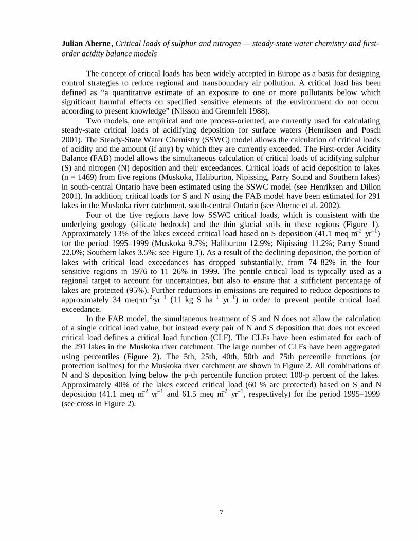
Julian Aherne , Critical loads of sulphur and nitrogen — steady-state water chemistry and first-order acidity balance models

The concept of critical loads has been widely accepted in Europe as a basis for designingcontrol strategies to reduce regional and transboundary air pollution. A critical load has beendefined as “a quantitative estimate of an exposure to one or more pollutants below whichsignificant harmful effects on specified sensitive elements of the environment do not occuraccording to present knowledge” (Nilsson and Grennfelt 1988).

Two models, one empirical and one process-oriented, are currently used for calculatingsteady-state critical loads of acidifying deposition for surface waters (Henriksen and Posch2001). The Steady-State Water Chemistry (SSWC) model allows the calculation of critical loadsof acidity and the amount (if any) by which they are currently exceeded. The First-order AcidityBalance (FAB) model allows the simultaneous calculation of critical loads of acidifying sulphur(S) and nitrogen (N) deposition and their exceedances. Critical loads of acid deposition to lakes(n = 1469) from five regions (Muskoka, Haliburton, Nipissing, Parry Sound and Southern lakes)in south-central Ontario have been estimated using the SSWC model (see Henriksen and Dillon2001). In addition, critical loads for S and N using the FAB model have been estimated for 291lakes in the Muskoka river catchment, south-central Ontario (see Aherne et al. 2002).

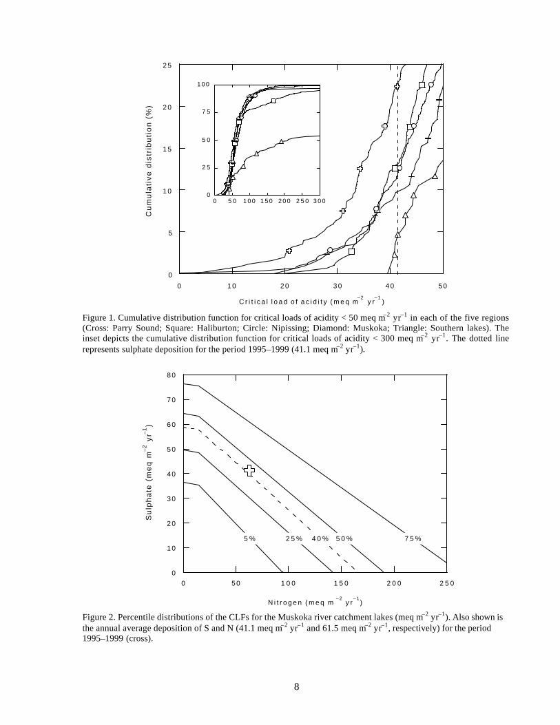
Four of the five regions have low SSWC critical loads, which is consistent with theunderlying geology (silicate bedrock) and the thin glacial soils in these regions (Figure 1).Approximately 13% of the lakes exceed critical load based on S deposition (41.1 meq m–2 yr–1)for the period 1995–1999 (Muskoka 9.7%; Haliburton 12.9%; Nipissing 11.2%; Parry Sound22.0%; Southern lakes 3.5%; see Figure 1). As a result of the declining deposition, the portion oflakes with critical load exceedances has dropped substantially, from 74–82% in the foursensitive regions in 1976 to 11–26% in 1999. The pentile critical load is typically used as aregional target to account for uncertainties, but also to ensure that a sufficient percentage oflakes are protected (95%). Further reductions in emissions are required to reduce depositions toapproximately 34 meq·m–2·yr–1 (11 kg S ha–1 yr–1) in order to prevent pentile critical loadexceedance.

In the FAB model, the simultaneous treatment of S and N does not allow the calculationof a single critical load value, but instead every pair of N and S deposition that does not exceedcritical load defines a critical load function (CLF). The CLFs have been estimated for each ofthe 291 lakes in the Muskoka river catchment. The large number of CLFs have been aggregatedusing percentiles (Figure 2). The 5th, 25th, 40th, 50th and 75th percentile functions (orprotection isolines) for the Muskoka river catchment are shown in Figure 2. All combinations ofN and S deposition lying below the p-th percentile function protect 100-p percent of the lakes.Approximately 40% of the lakes exceed critical load (60 % are protected) based on S and Ndeposition (41.1 meq m–2 yr–1 and 61.5 meq m–2 yr–1, respectively) for the period 1995–1999(see cross in Figure 2).

8

0

5

1 0

1 5

2 0

2 5

0 1 0 2 0 3 0 4 0 5 0

Cu

mu

lati

ve

dis

trib

uti

on

(%

)

C r i t i c a l l o a d o f a c i d i t y ( m e q m– 2

y r– 1

)

0

2 5

5 0

7 5

1 0 0

0 5 0 1 0 0 1 5 0 2 0 0 2 5 0 3 0 0

Figure 1. Cumulative distribution function for critical loads of acidity < 50 meq m–2 yr–1 in each of the five regions(Cross: Parry Sound; Square: Haliburton; Circle: Nipissing; Diamond: Muskoka; Triangle: Southern lakes). Theinset depicts the cumulative distribution function for critical loads of acidity < 300 meq m–2 yr–1. The dotted linerepresents sulphate deposition for the period 1995–1999 (41.1 meq m–2 yr–1).

0

1 0

2 0

3 0

4 0

5 0

6 0

7 0

8 0

0 5 0 1 0 0 1 5 0 2 0 0 2 5 0

N i t r o g e n ( m e q m– 2

y r– 1

)

Su

lph

ate

(m

eq

m–

2 y

r–1)

5 % 5 0 %2 5 % 7 5 %4 0 %

Figure 2. Percentile distributions of the CLFs for the Muskoka river catchment lakes (meq m–2 yr–1). Also shown isthe annual average deposition of S and N (41.1 meq m–2 yr–1 and 61.5 meq m–2 yr–1, respectively) for the period1995–1999 (cross).

9

Shaun Watmough, Acid deposition and the terrestrial environment

Acid deposition changed over time since pre-industrial times (1850s) to present. Higheracid deposition to catchments’ soils contributes to increased leaching of base cations and acid tosurface waters. Furthermore, tree harvesting is known to affect soil acidification by increasingthe uptake of base cations from soils.

The study presented has the objectives: (1) to determine whether soils inMuskoka/Haliburton are acidifying, (2) to identify factors responsible for soil acidification, (3)to develop (refine) models that predict the response of soils (and lakes) to acid deposition andharvesting. The study sites in Muskoka-Haliburtion regions have been monitored since the late1970s. These sites are particularly sensitive to acid deposition because they have shallow soils,low base saturation, and they receive high levels of acid deposition.

Mass balance studies were applied in seven representative sub-catchments in theMuskoka-Haliburton regions. Two of these (PC-1 and HP4) are discussed in more detail sincebaseline data is available since 1980s. At Plastic lake (PC-1), dominated by white pine andhemlock, there was no net base cation uptake between 1983 and 1999. At Harp lake (HP4),dominated by sugar maple, red maple and yellow birch there was a 20% increase in biomassbetween 1983 and 1999. At both catchments, Ca losses from soils to surface waters wereestimated using mass balances. Both catchments experienced Ca losses from soils to surfacewater and a decrease in soil pH in all soil horizons between 1982 and 1999.

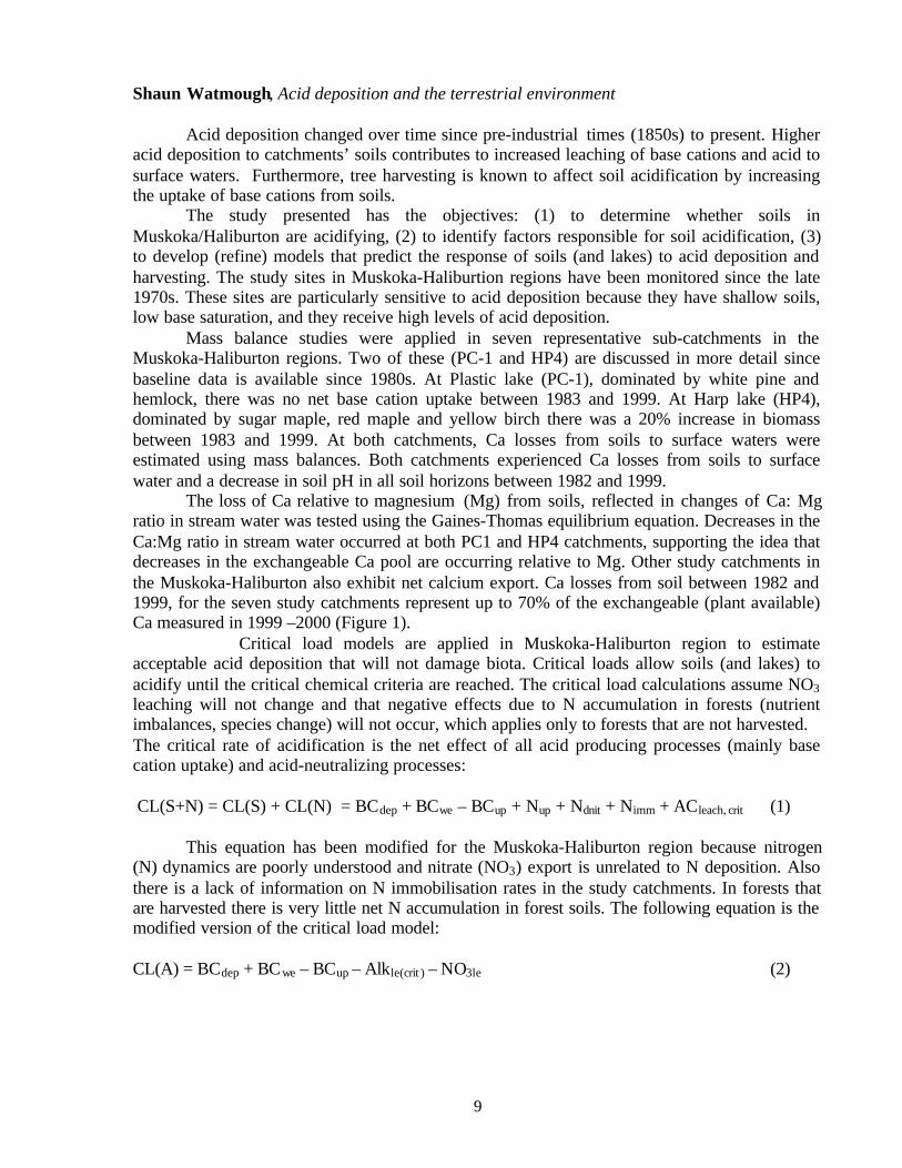
The loss of Ca relative to magnesium (Mg) from soils, reflected in changes of Ca: Mgratio in stream water was tested using the Gaines-Thomas equilibrium equation. Decreases in theCa:Mg ratio in stream water occurred at both PC1 and HP4 catchments, supporting the idea thatdecreases in the exchangeable Ca pool are occurring relative to Mg. Other study catchments inthe Muskoka-Haliburton also exhibit net calcium export. Ca losses from soil between 1982 and1999, for the seven study catchments represent up to 70% of the exchangeable (plant available)Ca measured in 1999 –2000 (Figure 1).

Critical load models are applied in Muskoka-Haliburton region to estimateacceptable acid deposition that will not damage biota. Critical loads allow soils (and lakes) toacidify until the critical chemical criteria are reached. The critical load calculations assume NO3

leaching will not change and that negative effects due to N accumulation in forests (nutrientimbalances, species change) will not occur, which applies only to forests that are not harvested.The critical rate of acidification is the net effect of all acid producing processes (mainly basecation uptake) and acid-neutralizing processes:

CL(S+N) = CL(S) + CL(N) = BCdep + BCwe – BCup + Nup + Ndnit + Nimm + ACleach, crit (1)

This equation has been modified for the Muskoka-Haliburton region because nitrogen(N) dynamics are poorly understood and nitrate (NO3) export is unrelated to N deposition. Alsothere is a lack of information on N immobilisation rates in the study catchments. In forests thatare harvested there is very little net N accumulation in forest soils. The following equation is themodified version of the critical load model:

CL(A) = BCdep + BCwe – BCup – Alkle(crit ) – NO3le (2)

10

Figure 1. Ca losses between 1982- 1999 relative to the present exchangeable Ca

There have been controversies over what constitutes an acceptable Alkle(crit ). In thecurrent study, Alkle(crit) has been set to zero, meaning that water draining the rooting zone will beallowed to acidify until the acid neutralising capacity ANC = 0 µeq/L, where ANC = (BCle –SO4

– NO3). The application of this critical load model to seven forested sub-catchments showed thatsites are much more sensitive to acid deposition if harvesting occurs and reductions in Sdeposition of approximately 50% are needed to prevent all 7 catchments to exceed the criticalchemical criteria (ANC = 0 µeq/L).

The mass balance studies showed that soils in the Muskoka-Haliburton region are stillacidifying despite reductions in S deposition and the losses of Ca through leaching andharvesting are of greatest concern. Mass balance studies are good predictors of base cationweathering. Harvesting has an enormous impact on the acid sensitivity of soils (and lakes),however harvest rates are poorly quantified at the study sites. If harvesting continues S leachingfrom soils must be reduced by up to 75% to prevent the ANC of water draining the rooting zonefalling to 0 µeq/L.

0

200

400

600

800

1000

1200

1400

1600

PC1 CB1 RC4 HP3A HP4 HP6 HP6A

Sub-Catchment

Ca

(kg

/ha

)

Ex-Ca in 1999/2000 Ca loss (1982-1999)

11

Keith Somers , Patterns in climate parameters. Understanding the role of climate signals

Over the last few years, we’ve realized that long-term patterns in water-quality andbiological parameters in Dorset-area lakes and streams are influenced by global, as well as localand regional factors. Historically our interests focused on local issues such as the impacts oflakeshore development on water quality (e.g., Dillon et al. 1994). The discovery of acidprecipitation broadened our studies to include a variety of regional factors to explain changes insulphate, pH and alkalinity (e.g., LaZerte and Dillon 1984). Most recently global climatesignals in the form of El Nino and La Nina events have been attributed to year-to-year variationin a number of water-quality parameters (Dillon et al. 1997). Consequently our interest in therole of climate signals has been growing.

There are a number of common perceptions about climatic factors and how they translateinto local weather events that directly affect Dorset-area lakes and streams. Clearly weatherpatterns vary markedly from year to year. It is generally accepted that El Nino periodscontribute to hot, dry summers, whereas La Nina events translate into cool, wet conditions in thenorthern hemisphere. El Nino events have been correlated with year-to-year variation in Dorsetwater-quality parameters such as sulphate (Dillon et al. 1997). Furthermore, El Nino has beenimplicated in affecting annual abundances of some zooplankton species (Rusak et al. 1999) andyear-class strength in fish species (Schindler 2001). However, linkages between Dorset-areaweather and global climate variables such as El Nino and La Nina (i.e., the Southern OscillationIndex or SOI), the North Atlantic Oscillation (NAO), and the Arctic Oscillation (AO) have notbeen established. Consequently, the growing evidence of the influence of climate signals onlong-term trends in chemical and biological parameters has sparked interest in a betterunderstanding of how climate signals affect local weather patterns.

Variability in the SOI is generally used to define El Nino and La Nina events. That is,extended periods of 6-or-more months of negative SOI values are often used to indicate an ElNino event and similar periods of positive values define La Nina events (Fig. 1). The periodspanning the Dorset-area data sets (i.e., 1978 to present) exhibits an increased frequency ofsignificant SOI events in the 1990s. For example, an El Nino event spanned the period fromMay 1991 to March 1995, although the anticipated hot, dry conditions were offset by theeruption of Mount Pinatubo in June 1991 and the influence of volcanic ash in the atmosphere.The subsequent period from January 1996 through March 2001 was characterized by a La Ninaevent that was briefly interrupted by an El Nino from March 1997 to April 1998. Clearly, the1990s provide an interesting contrast to the 1980s because there were only 2 El Nino events(May 1982 to Mar 1983 and November 1986 to February 1988) and 1 La Nina (July 1988 toJuly 1989) in the 1980s.

There is a variety of statistics that could be used to summarize the Dorset-area weather.In this preliminary investigation, I selected the mean average daily temperature from 4meteorological stations operated by the Dorset Environmental Science Centre. To shift alltemperatures (in oC) to positive values I added 40 and then summed the daily averages by monthto obtain an estimate of the total degree-days for each month and a total for each year. For eachmonth and the year total, I calculated the long-term mean for the period from 1979 to 2000. Tostandardize the results for each month, I subtracted the long-term mean from the observedmonthly value and then divided by the long-term mean. The resultant number multiplied by 100is the percent difference from the long-term mean. In the summary table (Fig. 2), I highlightedvalues that were more than 5% warmer than the long-term mean in green, and more than 5%colder in yellow.

Based on the annual total degree-day values, there were 3 cold years and 1 warm year inthe 1980s as compared to 4 cold years and 4 warm years in the 1990s (Fig. 2). The warmest year

12

was in 1998, whereas 1992 was the coldest year. The warmest year occurred during an El Ninoevent that began in March of 1997 and ran uninterrupted until April of 1998 (see Fig. 1). Thefollowing year, 1999, was also warmer than usual. Two relatively warm years were alsoobserved after the 1982-83 El Nino. However, 2 consecutive warm years were observed in1990-91 following a La Nina that started in July 1988 and ran through July 1989. As expected,the coldest year in 1992 followed the Mount Pinatubo eruption, and despite an extended El Ninothat ran from May 1991 through Mar 1995, the years from 1993 through 1997 were all colderthan the long-term average. After excluding the unusual events following the Mount Pinatuboeruption, there is a trend for the total degree-day temperatures in the year following the start ofan El Nino to be warmer, and the year following the start of a La Nina to be colder than thelong-term average. However, anomalous years such as 1990 and 1991 contradict thisgeneralization.

When the monthly values are examined, the months of June through October rarelyexhibit strong deviations from the long-term mean (Fig. 2). Over the 22 years, extreme valuesare most common in December, January and February. In some years, extreme values in onemonth are followed by extreme values in the opposite direction (e.g., January through April1995). These extremes tend to cancel each other out in the annual total (e.g., 1979 and 1995)suggesting that modeling climate data with monthly values may prove to be more rewardingthan using annual totals.

This preliminary analysis using monthly total degree-days indicates that there isconsiderable variability in the Dorset average air-temperature data. However, linkages betweenair temperature and the SOI are weak, perhaps because of the relatively short duration of thedata set (i.e., 22 years) and the substantial impact of the Mount Pinatubo eruption. Theobservation that total degree-days were relatively invariant from June through October, but quitevariable in December, January and February suggests that temperature extremes in these wintermonths may be very important for explaining year-to-year variation in biological and water-quality variables. This latter hypothesis will be evaluated in our future analyses.

13

Figure 1. Southern oscillation index (SOI) values by month from 1978 to 2001 with El Nino periods highlighted ingreen and La Nina events in yellow. El Nino years are indicated in red and the Mount Pinatubo year is indicated inblue.

Figure 2. Monthly total degree-days as a percent deviation from the long-term mean. Values colder than 5% arehighlighted in yellow, whereas values warmer then 5% are highlighted in green. The right-most column is thepercent difference based on the total degree-days for each year. In this column, years that are more than 1%warmer than the long-term average are highlighted in green and years that are more than 1% colder are highlightedin yellow. Red values in the left-most column indicate El Nino events and the blue value indicates the year thatMount Pinatubo erupted.

Year Jan Feb Mar Apr May Jun Jul Aug Sep Oct Nov Dec

1978 -0.4 -3.5 -0.8 -0.6 1.3 0.3 0.4 0 0 -0.7 -0.1 -0.31979 -0.7 0.8 -0.5 -0.4 0.3 0.4 1.3 -0.6 0.1 -0.4 -0.6 -1

1980 0.3 0 -1.2 1 -0.3 -0.4 -0.2 0 -0.6 -0.3 -0.5 -0.3

1981 0.2 -0.6 -2.1 -0.4 0.7 1 0.8 0.4 0.4 -0.7 0.1 0.5

1982 1.3 -0.1 0.1 -0.2 -0.7 -1.6 -1.9 -2.5 -2 -2.2 -3.2 -2.81983 -4.2 -4.6 -3.4 1.3 0.5 -0.3 -0.8 -0.2 1 0.3 -0.2 -0.1

1984 0.1 0.6 -0.9 0.2 0 -0.8 0 0 0.1 -0.6 0.2 -0.4

1985 -0.5 1 0.2 1 0.2 -0.9 -0.3 0.7 0 -0.7 -0.3 0.1

1986 0.9 -1.6 0 0.1 -0.5 0.7 0.1 -1 -0.6 0.5 -1.5 -1.8

1987 -0.9 -1.9 -2 1.9 -1.7 -1.7 -1.7 -1.5 -1.2 -0.7 -0.1 -0.71988 -0.2 -0.9 0.1 -0.1 0.8 -0.2 1.1 1.4 2.1 1.4 1.9 1.3

1989 1.7 1.1 0.6 1.6 1.2 0.5 0.8 -0.8 0.6 0.6 -0.4 -0.7

1990 -0.2 -2.4 -1.2 0 1.1 0 0.5 -0.6 -0.8 0.1 -0.7 -0.5

1991 0.6 -0.1 -1.4 1 -1.5 -0.5 -0.2 -0.9 -1.8 -1.5 -0.8 -2.31992 -3.4 -1.4 -3 1.4 0 -1.2 -0.8 0 0 -1.9 -0.9 -0.91993 -1.2 -1.3 -1.1 -1.6 -0.6 -1.4 -1.1 -1.5 -0.8 -1.5 -0.2 0

1994 -0.3 -0.1 -1.4 1.8 -1 -0.9 -1.8 -1.8 -1.8 -1.6 -0.7 -1.6

1995 -0.6 -0.5 -0.2 1.1 -0.7 -0.2 0.3 -0.1 0.3 -0.3 0 -0.8

1996 1 -0.1 0.7 0.6 0.1 1 0.6 0.4 0.6 0.4 -0.2 0.8

1997 0.5 1.6 -1.1 -0.9 -1.8 -2 -1 -2.1 -1.6 -1.9 -1.4 -1.31998 -3.3 -2.7 -3.5 -1.9 0.1 0.7 1.3 1 1.2 1 1.1 1.4

1999 2 0.8 0.9 1.4 0.1 -0.1 0.5 0.1 -0.1 0.9 1.1 1.5

2000 0.7 1.6 1 1.2 0.2 -0.6 -0.4 0.4 1 1 2 0.7

2001 1.1 1.5 0.5 -0.1 -0.8 -0.1 -0.4 -1 0.2 -0.4 0.7 -1.2

Year Jan Feb Mar Apr May Jun Jul Aug Sep Oct Nov Dec % Diff.

1979 -8.7 -20.5 6.2 0.6 1.4 1.3 1.3 -0.8 1.6 0.4 5.1 4.7 0.08

1980 3.2 -9.1 -4.9 1.7 1.6 -5.6 0.5 3.6 -0.6 -3.4 -3.0 -18.1 -2.21

1981 -18.1 12.6 0.1 2.7 -2.2 -0.1 0.0 0.3 -0.8 -3.1 1.5 1.9 -0.42

1982 -19.0 -7.1 -4.5 -6.2 5.7 -2.5 0.2 -3.3 1.1 4.4 4.7 12.1 -0.69

1983 6.5 6.3 3.3 -1.6 -5.1 0.5 1.6 3.3 4.4 1.0 0.7 -10.1 0.82

1984 -7.9 19.3 -10.8 3.8 -4.9 1.4 -0.9 2.4 -2.3 5.1 0.1 8.1 0.73

1985 -8.1 2.1 0.8 -1.4 0.1 -3.7 -1.6 -1.5 1.6 2.0 -0.1 -6.7 -1.21

1986 0.3 -3.6 2.6 5.9 3.4 -2.3 0.4 -2.4 -1.0 -0.5 -3.5 7.2 0.43

1987 9.0 -2.2 5.8 8.3 2.2 2.0 3.1 -0.1 2.0 -3.9 0.4 9.4 2.69

1988 -1.9 -1.7 2.8 -2.5 -3.2 -2.7 3.8 2.2 -0.2 -5.0 4.7 0.1 -0.24

1989 13.8 -5.7 -5.0 -4.4 0.4 1.0 1.7 0.0 0.0 1.4 -3.3 -24.7 -1.60

1990 21.8 4.6 0.6 2.8 -2.8 0.7 0.3 1.1 -1.4 -0.2 0.9 4.1 1.86

1991 0.8 5.2 3.1 3.8 5.8 3.0 0.5 1.9 -2.2 2.7 -0.2 -0.9 1.94

1992 1.8 2.8 -8.9 -3.8 -0.5 -3.1 -5.6 -3.9 -0.5 -4.3 -1.9 3.7 -2.44

1993 6.8 -16.0 -2.5 -0.1 -0.9 -1.3 0.7 1.6 -3.9 -3.3 -2.0 -0.6 -1.50

1994 -25.7 -12.9 -1.1 -0.6 -2.2 1.3 -0.3 -2.9 0.2 1.5 4.5 6.7 -1.78

1995 14.5 -10.1 5.6 -6.6 -0.6 3.9 0.3 2.3 -3.5 3.8 -7.8 -9.7 -0.44

1996 -2.9 -1.3 -5.2 -5.8 -2.8 1.6 -2.8 0.5 1.9 0.3 -5.6 10.3 -0.99

1997 -3.7 1.7 -1.8 -4.0 -7.3 2.8 -1.1 -2.4 -1.0 -0.5 -1.5 3.4 -1.40

1998 14.1 16.4 3.3 3.4 7.3 0.8 -0.9 1.3 2.5 1.9 3.2 8.3 4.17

1999 0.7 8.2 0.9 2.6 5.2 3.1 1.8 -1.8 2.8 -2.6 2.4 2.4 1.96

2000 2.7 11.0 9.7 1.2 -0.9 -2.1 -2.8 -1.4 -0.6 2.3 0.7 -11.5 0.22

Average 917 890 1149 1333 1592 1678 1816 1777 1584 1443 1205 1035

14

Jim Buttle, Thresholds influencing slope – riparian zone – stream coupling: an example fromthe Canadian Shield

Hydrologists have long-recognized the nonlinear response of basin runoff to input, andthe role that the variable interaction between input characteristics and basin antecedent wetnessplays in contributing to this nonlinearity. This interaction is incorporated into several currentsemi-distributed hydrological models (e.g. TOPMODEL, TOPOG-SBM) that explicitly considerthe role of basin morphology in influencing streamflow generation. Nevertheless, such modelsgenerally fail to capture the complex manner in which input and antecedent wetnesscharacteristics control spatial and temporal patterns of hydrologic coupling between slopes,riparian zones and streams, even in basins with relatively “simple” morphologies. We examinethe nature of hydrologic coupling based on the results of long-term studies of streamflowgeneration at point-, slope- and basin-scales in the PC1-08 basin on the Canadian Shield insouth-central Ontario.

The topography (two near-linear slopes draining to riparian zone located in mini-grauben) of PC1-08 results in an abrupt physical limit to the maximum spatial extent of theriparian zone. This means that major changes in basin runoff response to input must involveslope contributions. These slopes have very similar surface morphologies; however, there aremarked differences between the surface and bedrock topography in a number of locations in thebasin. Measurements of runoff from instrumented slope elements indicate that the propensity ofa particular slope to contribute runoff seems to depend (at least initially) on soil depth. Thus,areas of thin or no soil cover almost always generate a runoff response, while slope elementswith deeper and more variable soil cover have a more nonlinear runoff response to rainfall thatshuts down completely during mid-summer when the basin is at its driest. The morepronounced seasonal variability in the ability of slope elements with deeper soil cover togenerate runoff may reflect the presence of bedrock depressions, the variable storage of water inthese depressions, and the need to link these depressions hydrologically in order to generatesignificant slope runoff. Critical thresholds of both input depth and of antecedent wetness mustbe surpassed in order to link up saturated bedrock depressions such that these slope elements cancontribute runoff to the riparian zone. Whether these slope runoff fluxes actually contribute tobasin runoff response depends on the control of antecedent wetness on water table conditions inthe riparian zone. A continuous water table along the length of the stream valley both beforeand during an event is required to generate significant stormflow at the basin scale in PC1-08.Sustained conditions of high water tables along the length of the riparian zone are most commonin late spring and fall. Field observations indicate that they can occur during mid-summer, butonly in response to exceptionally-large rainfall inputs.

This empirically-based approach has identified some of the critical thresholds (in termsof event size, soil depth, and riparian zone groundwater volume) that need to be exceeded inorder to generate significant stormflow at the basin scale. Knowing if and when runoff fluxesfrom slopes and from basins will occur is important to our understanding of the transport of suchcompounds as DOC and SO4 to receiving wetlands and lakes. Our work on slopes suggests thatsoil distribution on basin slopes in PC1-08 exerts powerful control on whether slope elementswill generate runoff that will be delivered to the stream valley. The thickness and variability ofsoil depth on a slope also appears to influence its degree of sensitivity to antecedent wetnessconditions, such that shallow soil slopes are not very sensitive while slopes with deep andvariable soils tend to be highly sensitive. At the same time, the interaction between antecedentwetness and the soil distribution in the stream valley controls whether these runoff contributionsfrom the basin slopes will result in the generation of basin-scale stormflow. Current modelsbased on surface topography cannot capture the influence that the distribution of soil thickness

15

plays in stormflow generation in Shield basins like PC1-08. Progress in this area will requirethe identification of the point at which divergence between surface topography and bedrocktopography can lead to incorrect predictions from topographically-based hydrological models, aswell as improvements in our ability to estimate bedrock topography.

16

Catherine Eimers, Sources and Controls of Sulphur Cycling in Muskoka-HaliburtonCatchments

Long-term (~20-year) sulphate (SO4) mass balance budgets were calculated for a numberof catchments in the Muskoka-Haliburton region. Results indicated that (1) temporal patterns ofSO4 chemistry in stream water are synchronous among catchments and (2) all catchments exportmore SO4 in stream water than is input in bulk deposition in certain years, resulting in anapparent net export of SO4.

Synchronous patterns of SO4 chemistry across a range of catchments indicate that largescale or regional factors are involved. Two factors that act on a sufficiently broad scale andcould therefore be responsible for synchronous patterns of SO4 chemistry are deposition andclimate. Inter-annual changes in stream SO4 concentrations were not strongly related to temporalchanges in deposition, but were highly correlated with catchment dryness. Specifically, SO4

concentrations were higher and SO4 export from catchments was greater in years when streamflow ceased completely. The number of days with zero stream flow was generally a function ofsummer precipitation and temperature. The effects of drying and re-wetting and temperature onSO4 release in wetland and upland material are shown in Figures 1 and 2. These results indicatethat changes in climate should be considered when attempting to interpret the response ofcatchments to changes in deposition.

The second observation of net SO4 export was calculated using the following equation:

Stream export – Deposition + Weathering = Net Change (retention/export) (1)

By comparing stream export with bulk deposition only, annual net SO4 export from the uplanddraining PC1-08 catchment was calculated to range from 8 to 28 kg/ha/yr (average:approximately 20 kg/ha/yr), while export from the wetland-draining PC1 catchment ranged from–4 to 30 kg/ha/yr (average: approximately 13 kg/ha/yr). Even if weathering is assumed tocontribute 2 kg SO4/ha/yr (value estimated for the Hubbard Brook) and bulk deposition inputsare increased by an additional 20% to account for potentially unmeasured dry deposition, netexport from catchments is still large and is around 14 kg/ha/yr in PC1-08 and 8 kg/ha/yr in PC1,respectively. Net SO4 export from catchments must therefore be due to release from internalpools, which will delay the response of catchments to changes in deposition.

17

Figure 1. Sulphate release from PC1 wetland: effect of drying and temperature

Figure 2. Sulphate release from PC1-08 upland: effect of drying and temperature

wet

dry

0

100

200

300

PEAT SPHAGNUM

SO

4 r

ele

as

e (

mg

/kg

)

18/wet

25/wet

18/dry

25/dry

wet dry

0

100

200

300

400

500

600

LITTER MINERAL SOIL

SO

4 r

ele

as

e (

mg

/kg

)

18/wet

25/wet

18/dry

25/dry

18

Peter Dillon, Lake Mass Balances

Lake mass balances are currently used in several studies (Devito and Dillon 1989, Molotand Dillon, 1996) to calculate lake budgets for various substances such as carbon, nitrogen, andalkalinity. Mass balances are measured (1) to assess the relative importance of sources (such asatmosphere and terrestrial catchment) of a substance to lakes and/or catchments, (2) to modellake or catchment response to changes in parameters (e.g. input rates), and (3) to identifyimportant processes in lakes and catchments. For example, for sodium (Na) and chloride (Cl)budgets can be calculated from the equation:

TERRin + ATMin + ÄS = OUT (1)

In this case the sedimentation rate constant (í) is zero. For substances such as iron, which playsan important role in the cycling of nutrients such as P, trace metals, DOC and sulphur,sorption/desorption processes to/from lake sediments occur, and the following mass balanceequation is used:

TERRin + ATMin + REL+ ÄS = OUT + SED (2)

Where REL = release from sediments to lake, and SED = sorption to sediments from the watercolumn. For gaseous forms, such as DIC, Hg, their budgets are calculated as follows:

TERRin + ATMin + REL+ ÄS = OUT + SED + ATMout (3)

For a number of lakes in the Muskoka river catchment, budgets for alkalinity, carbon,nitrate (NO3), ammonia, organic nitrogen and total inorganic nitrogen (TIN) were calculatedusing the mass balance approach. Alkalinity is typically influenced by the redox processes inlakes (i.e. reduction processes produce alkalinity, while oxidation processes consume alkalinity).The reduction of FeIII, sulphate and nitrate is an important alkalinity generating mechanism inlakes. For example, the alkalinity budget for Plastic Lake is shown in Table1.

Table 1. Plastic lake alkalinity budget

In the calculation of carbon budgets in lakes, processes such as degassing (loss of CO2

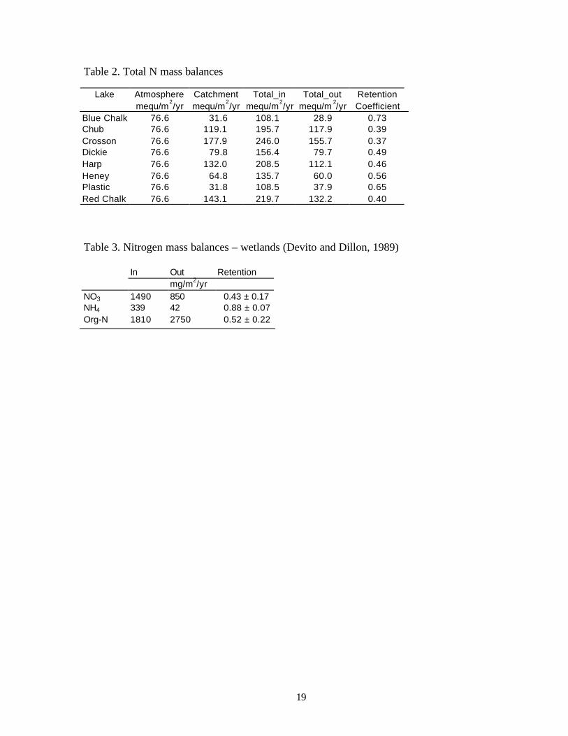
to the atmosphere) and loss to sediments are important. At Dickie lake, a much higher Cretention in sediments was computed relative to Plastic Lake (10.1 and 2.2 g C/m2/yr,respectively). Also, the CO2 degassing (mg/m2 /day) at Dickie Lake was approximately fivetimes higher than at Harp Lake. These budgets are likely to reflect differences in input sourcesand internal processes for different lakes. For calculating nitrogen budgets in lakes, in-lakeremoval processes such as denitrification in the anoxic sediment, uptake by primary producersand particulate sedimentation are important. For example, total N mass balances for eightMuskoka catchments are shown in Table 2 and N mass balances computed for wetlands (Devitoand Dillon, 1989) are displayed in Table 3.

Internal ProcessesNO3

- loss 33

NH4+ loss -22

SO42- reduction 70

Total 81

Plastic Lake Alkalinity meq/m2/yr

External Input 155Output 14Difference = Lake processes 169

19

Table 2. Total N mass balances

Table 3. Nitrogen mass balances – wetlands (Devito and Dillon, 1989)

In Out Retentionmg/m2/yr

NO3 1490 850 0.43 ± 0.17NH4 339 42 0.88 ± 0.07Org-N 1810 2750 0.52 ± 0.22

Lake Atmosphere Catchment Total_in Total_out Retentionmequ/m

2/yr mequ/m

2/yr mequ/m

2/yr mequ/m

2/yr Coefficient

Blue Chalk 76.6 31.6 108.1 28.9 0.73Chub 76.6 119.1 195.7 117.9 0.39Crosson 76.6 177.9 246.0 155.7 0.37Dickie 76.6 79.8 156.4 79.7 0.49Harp 76.6 132.0 208.5 112.1 0.46Heney 76.6 64.8 135.7 60.0 0.56Plastic 76.6 31.8 108.5 37.9 0.65Red Chalk 76.6 143.1 219.7 132.2 0.40

20

Sherry Schiff, Dissolved Organic Matter, What can isotopes tell us?

Dissolved organic matter (DOM) is important in various aspects of geochemistry, oftencontrolling pH, alkalinity/acid buffering capacity, and metal binding and solubility in softwatersystems. DOM has also a large role in ecology. In aquatic systems, DOM is an importantmicrobial food source, and has a major role in the transport and toxicity of trace metals andother contaminants. Furthermore, DOM controls the heat and light levels in lakes with itsinfluence on colour/light extinction, heat budget and UV penetration. DOM is a mixture of alarge number (103) of compounds, and it is highly variable spatially and temporally. Carbonisotopes are typically used in research studies to examine the sources of carbon, such asgroundwater, surface waters, stemflow, throughfall, litter, soils and wetlands. Isotopes arechemically similar, but have different atomic mass and their ratios (e.g 13C/12C) are measuredrelative to a standard (O ‰). Carbon has three naturally occurring isotopes 12C, 13C, and 14C.Typical aquatic DOM is made of 53% C, 40.5% O, 4.6% H, 1.3% N, and 0.8% S. Some of theisotopic ratios that can be analyzed in DOM are 14C/12C, 13C/12C, 18O/16O, 15N/14N, 34S/32S.

A number of studies were conducted at Harp catchment, located on the PrecambrianShield (Schiff et al., 1998, Schiff et al., 1997) to measure 14C in upland and wetland catchments.In upland catchments, such as Harp-21 devoid of wetlands, 14C in DOC was found to be lessthan 0 ‰, similar to groundwater values, suggesting that groundwaters may be important DOCsources in upland streams. Values of 14C higher than 80 ‰ in most streams of Harp Lakecatchment indicate that most DOC has been exported to stream within the last 40 years (Schiff etal., 1990). In streams out flowing from wetlands, values of 14C over 50 ‰ were recorded. Thelower values observed in the inflows to Harp Lake corresponded to periods when the streamdischarge was low. In this case, the stream water sources were areas adjacent to stream, where athick deposit of glacial lacustrine silts and clays slowly released stored groundwater of low 14Cvalues (Schiff et al., 1997).

Other isotopes such as 13C can also be used to identify sources of carbon within awatershed. The 13C composition is similar to the predominant plants in the watershed (C3 plantsare characterised by �13C values ranging between –25 ‰ and –30 ‰, while C4 plants arecharacterised by �13C values ranging between –8 ‰ and –13 ‰). Current research is focused onidentifying and understanding temporal variations of 13C/12C relative to 15N/14N within awatershed. Also, isotopes such as 14C, 13C, 15N and 34S/ 32S are investigated to determine sourcesof DOM in soil and groundwater, and metal binding properties within DOM.

21

Julian Aherne , MAGIC — simulating drought induced sulphate peaks in stream chemistry atPlastic Lake

One of the principal influences on the flux of many elements from forested catchments inOntario is the atmospheric deposition rate of strong acids. While sulphate deposition hasdecreased ca. 45% in the past two decades, nitrate deposition has remained unchanged and nowequals sulphate deposition. Sulphate concentrations in headwater lakes and their inflows havedecreased, but much less than expected based on the anticipated direct response of thecatchments. In Plastic Lake, the decrease has been 21%. While for others, the decrease has beeneven lower. As a further consequence, alkalinity and pH recovery has been slow. Redoxprocesses occurring in wetlands have been identified as the reason for delayed recovery, andclimate events, particularly the El Niño phenomenon, as controlling these redox processes.

A new version of the biogeochemical model MAGIC (Model of Acidification ofGroundwater In Catchments) that incorporates wetlands and redox processes driven by climateevents has been generated, and model predictions show good agreement with fieldmeasurements for Plastic Lake. MAGIC is a lumped-parameter model of intermediatecomplexity, developed to predict the long-term effects of acidic deposition on soils and surfacewater chemistry. MAGIC has been in use for 15 years and has been applied extensively in NorthAmerica and Europe. Several refinements or additions to MAGIC have been proposed orimplemented over the years as a result of the many applications of the model, e.g., the wetlandredox module. The model simulates soil solution chemistry and surface water chemistry topredict monthly and annual average concentrations of the major ions in lakes and streams.MAGIC represents the catchment with aggregated, uniform soil compartments (one or two), awetland compartment (new module, which has only been applied to Plastic Lake to date) and asurface water compartment that can be either a lake or a stream. Soil layers can be arrangedvertically or horizontally to represent flowpaths through the soil. The main drivers of the modelare time series inputs of major ion depositions (hindcasts and forecasts), discharge volumes andbiological production, removal and transformation. In addition, the model requires physical andchemical characteristics of the soil, wetland and surface water. The model is calibrated usingobserved values of surface water and soil chemistry for a specific period. Typically, modelledand observed values are brought into agreement by adjusting parameters such as weathering,initial base saturation and aluminium solubility constant.

The Plastic Lake simulation was set up with a soil, wetland and stream compartments.The soil compartment represents an orthic ferro-humic podzol, with an average depth of 0.35 mand cation exchange capacity of 35 meq kg–1. The wetland compartment represents a humicmesisol, which covers approximately 7% of the catchment, with an average depth of 1.0 m. Adischarge threshold is set for the wetland (Q threshold), when discharge is less than thethreshold then sulphur oxidation occurs. When discharge is greater than the threshold thenreduction occurs (currently not implemented in the Plastic Lake application). The threshold wasset at 1.5 cm month–1 for Plastic Lake. Calibration was carried out by comparing approximately20 years of measured stream chemistry with modelled stream chemistry. Reasonable agreementbetween measured and modelled stream concentrations was obtained for sulphate (see Figure 1).Differences between modelled and measured concentrations occur during periods of no-flow,e.g., see sulphate during summer 1990. As no flow was observed, no concentration wasmeasured. However, MAGIC requires a minimum flow, as such, MAGIC simulates a highconcentration due to the low simulated flow. Reasonable agreement between measured andmodelled stream fluxes was also obtained for sulphate (see Figure 1).

22

0

200

400

600

800

1000

1200

1400

Jan-80 Jan-81 Jan-82 Jan-83 Jan-84 Jan-85 Jan-86 Jan-87 Jan-88 Jan-89 Jan-90 Jan-91 Jan-92 Jan-93 Jan-94 Jan-95 Jan-96 Jan-97

Su

lph

ate

co

nce

ntr

ati

on

(µ

eq

L–1 )

56

Figure 1. Measured (circle) and modelled (square) sulphate stream concentrations at Plastic Lake for the period 1980–1997.

0

5

10

15

20

25

30

35

40

45

50

Jan-80 Jan-81 Jan-82 Jan-83 Jan-84 Jan-85 Jan-86 Jan-87 Jan-88 Jan-89 Jan-90 Jan-91 Jan-92 Jan-93 Jan-94 Jan-95 Jan-96 Jan-97

Su

lph

ate

flu

xes

(me

q m

–2 y

r–1)

5

6

Figure 1. Measured (circle) and modelled (square) sulphate stream fluxes at Plastic Lake for the period 1980–1997.

Mismatches between summer peaks do not occur as described above, e.g., see sulphate summer 1990 in Figure 1b. However, the dynamicsof spring runoff have not been correctly parameterised in the model. MAGIC does not differentiate between snow and precipitation; hence, itdoes not accumulate snow over the winter period to simulate a large peak in runoff during spring-melt. This can be corrected by portioningprecipitation inputs during the winter months to the months they are hydrologically active (currently in progress). In summary, MAGICadequately captures the sulphate peak after periods of drought by simulating sulphur oxidation pulses from the wetland at Plastic Lake.

23

Dean Jeffries, Recovery of aquatic ecosystems in south eastern Canada from acidic deposition

Emissions of Sulphur Dioxide. Eastern Canadian emissions of SO2 remained relativelyconstant from 1994 to 1997. In 1997, emissions of SO2 in the seven easternmost provincesremained 24% below the target of 2.3 million tonnes. Smelting of metal ores, the largestemission source in Canada, accounted for 49% of total eastern Canadian SO2 emissions in 1997.Power generation and other sources contributed 21% and 30%, respectively. Canada met itsgoal of limiting annual national SO2 emissions to 3.2 million tonnes in 1992. By 1995, its SO2

emissions were down to approximately 2.7 million tonnes, a 42% reduction from the 1980 levelof 4.6 million tonnes. Total U.S. emissions of SO2 fell by about 13% between 1993 and 1996,from 19.9 million tonnes to 17.4 million tonnes. Electric utilities are the largest source of U.S.SO2 emissions, accounting for 66% of total emissions in 1996. The United States is committedto reducing its annual SO2 emissions to 14.5 million tonnes by the year 2000, 9.1 million tonnesbelow 1980 levels. (Information for this item and some others below from the NationalEnvironmental Indicator Series, http://www.ec.gc.ca/soer-ree/English/Indicators/default.cfm).

Emissions of Nitrogen Oxides. In Canada, NOx emissions remained around the 2million tonne level over the 1991–95 period. Mobile sources (e.g., cars, trucks, rail, air, andmarine transportation) accounted for 52% of total Canadian NOx emissions in 1995, whilestationary sources (e.g., power generation, industrial processing, commercial and residentialcombustion) accounted for the remainder. Total U.S. NOx emissions fell by 4% between 1993and 1996, from 22.3 million tonnes to 21.3 million tonnes. Canadian measures to reduce mobileNOx emissions include more stringent performance standards on exhaust emissions from newvehicles, whereas measures to reduce stationary source emissions include emission limits fornew fossil-fuelled power plants, retrofits at several existing power plants, and new standards forboilers, process heaters, and kilns. Under the Canada–United States Air Quality Agreement,Canada is committed to a 10% reduction in projected NOx emissions (of 970 000 tonnes) fromstationary sources by the year 2000. The United States must reduce its total annual NOx

emissions by approximately 1.8 million tonnes from the 1980 level by the year 2000.

Wet Sulphate Deposition. The area in eastern Canada receiving 20 kg/ha/year or moreof wet sulphate deposition declined by 61% between the two five-year periods, 1980–84 and1991–95, reflecting the reduction in SO2 emissions in both Canada and the United States. The20 kg/ha/year wet sulphate deposition target was established as an interim objective in the1980s. Recent research confirms that this target is too high, as 20 kg/ha/year exceeds thebuffering capacity of many acid-sensitive lakes in eastern Canada. The temporal pattern in bulksulphate deposition at the Turkey Lakes Watershed and Dorset are displayed in Figure 1. Thecritical load for aquatic ecosystems is the amount of wet sulphate deposition that must not beexceeded in order to protect at least 95% of lakes in a region from acidifying to a pH level ofless than 6.0. Many studies suggest that a pH of at least 6.0 is needed to protect most aquaticorganisms. Scientists predict that large areas in eastern Canada, encompassing tens of thousandsof lakes, will continue to receive wet sulphate deposition above critical load limits for aquaticecosystems, even after the Canadian and U.S. SO2 emission controls are fully implemented inthe year 2010.

24

Figure 1. Annual bulk sulphate deposition measured at the Turkey Lakes Watershed and Dorset. Both sites exhibitstatistically significant declining trends.

Figure 2. Exceedance of wet sulphate deposition above critical loads

Trends in lake acidity in south-eastern Canada (1981-1997). Of 152 lakes monitoredfor acid rain effects in Ontario, Quebec, and the Atlantic Region between 1981 and 1997, 41%showed some improvement in acidity. Acidity levels were stable in 50% of the lakes andbecame worse in 9% (Figure 3). Seventy-three percent of the monitored lakes in Ontario are inthe Sudbury region. Improvements in most of the lakes in the Sudbury area can be attributed tothe substantial control of SO2 emissions from local nickel smelters. Despite significant SO2

controls in all of eastern Canada, the acidity of most lakes in the rest of Ontario, Quebec and theAtlantic Region shows little change partly because of the continuing transboundary flow ofacidifying emissions from the United States. Lake sulphate levels are indicators of the primaryacidifying agent (sulphuric acid) in acid rain. Sulphate levels are declining in most lakes inOntario, Quebec, and the Atlantic Region (Figure 3). Lake sulphate levels respond to areduction in SO2 emissions. A time lag of many years is possible before this translates into

0

200

400

600

800

1 000

1 200

1 400

1980 1982 1984 1986 1988 1990 1992 1994 1996

Are

a (K

m2, 0

00

s)

25

widespread regional improvements in lake pH or alkalinity. There is a further time lag beforethese improvements are likely to result in changes to populations of fish and other biota.

Figure 3. Chemical trends (expressed as a percent of monitored lakes) occurring over the 1981-97 time period fromthree regions of south eastern Canada. “Improving” trends were increasing pH and/or alkalinity for acidity anddeclining sulphate. “Worse” trends were declining pH and/or alkalinity for acidity and increasing sulphate.“Stable” indicates that no statistically significant trends were detected.

Analyses of chemical trends in Ontario using data sets that are more representative of the overalllake population (than that presented in Figure 3 which is heavily weighted by Sudbury data)show that declining sulphate and increasing pH/alkalinity were not so predominant during the1990s. The Ontario trends were influenced by drought, which acted to mobilize sulphate storedin wetlands and delay acidity improvements.

26

Bill Keller, Recovery of Acidified Lakes near Sudbury, Ontario, Canada

Over 7000 lakes in a 17,000 km2 area around Sudbury, Ontario, Canada were acidified topH < 6.0 by sulphur deposition associated with emissions from the Sudbury area metal smelters(Neary et al. 1990). Pollution controls implemented in the 1970's and 1990's have resulted inabout a 90% overall reduction in sulphur emissions from the smelters since peak years in the1960's. Emissions of metal particulates have been similarly reduced.

Emissions reductions have resulted in large changes in the chemistry of Sudbury arealakes, including increased pH and decreased concentrations of sulphate, base cations, andaluminum (Keller et al. 1992) (Figures 1, 2, and 3). While chemical improvements have beensubstantial in some lakes, many are still severely acidified, although recovery is continuing. Asthe Sudbury sulphur emissions have been reduced over the years, the relative effects of the longrange transport and deposition of sulphur have become more important in this area, and nowappear to dominate inputs to many lakes. Additional monitoring will be needed to determine thelong-term chemical responses of lakes around Sudbury to reduced acid deposition.

With improving water quality, biological recovery has been observed in some lakes,among various groups of organisms including fish, zooplankton, phytoplankton and benthos, butgenerally biological recovery is still at an early stage (Gunn and Keller 1990; Keller et al. 1999).Studies of Sudbury lakes are, however, beginning to yield an understanding of chemical andbiological lake recovery processes at a time when evidence of aquatic recovery fromacidification is only starting to emerge from other acid-affected areas of the world.

As studies of the lakes around Sudbury have progressed, it has become apparent that thechemical and biological recovery of these lakes from acidification is also closely linked to theeffects of other major environmental stressors. Extremely clear and acidic lakes became muchclearer in recent decades, probably because of climate change and solar bleaching, even thoughthey were slowly decreasing in acidity (Gunn et al. 2001). Such clear lakes in the Sudbury areaappear to have substantially increased UV-B penetration depths in comparison to pre-industrialconditions (Keller et al., under review) (Figure 4). The thermal structure of lakes near Sudburywas found to differ substantially between warm and cold years, with quite different responses inclear and colored lakes. Clear lakes, including many acid lakes, appear to be particularlysensitive to the effects of warming by climate change (Snucins and Gunn 2000). Given theirproximity to the Great Lakes, the potential for invasions by exotic species that have colonizedthe Great Lakes is also of concern for lakes in the Sudbury area. To date, the spiny waterflea(Bythotrephes cederstroemi) has been detected in a number of Sudbury area lakes. Otherinvaders may follow.

Drought results in oxidation of reduced sulphur stored in lake catchments and sedimentsfrom years of elevated atmospheric deposition. Remobilization of this stored acidity under wetconditions has resulted in delayed recovery or even re-acidification of some Sudbury lakes aswell as many related physical and chemical changes including metal mobilization, changes inthermal structure, and increased UV-B penetration (Keller et al. 1992; Yan et al. 1996). Suchreacidification events can have severe consequences for the biological recovery of lakes (Arnottet al. 2001) which we are only beginning to understand.

Monitoring programs have shown that concentrations of calcium have decreased inSudbury area lakes during the last two decades, apparently due to reduced acid leaching ofwatersheds as acid deposition was reduced (Figure 3). Other factors including climate changes,reduced calcium deposition from the atmosphere, and forest harvesting may, however, also beinvolved in the calcium declines (Keller et al. 2001). Current calcium concentrations appear tobe substantially lower than pre-industrial concentrations inferred from diatom remains in lakesediments. Calcium declines have biological as well as chemical implications since some

27

important organisms have relatively high calcium requirements, and calcium concentrations canmodify the effects of environmental stressors like acid and metals. It is apparent that futurestudies of acid-damaged lakes around Sudbury and elsewhere will need to be conducted in thecontext of multiple interacting stresses.

Figure 1. Plots of summer pH values for eight Killarney Park (40-60 km southwest of Sudbury) monitoring lakes,1981-2001

Figure 2. Plots of summer sulphate values for eight Killarney Park (40-60 km southwest of Sudbury) monitoring

lakes, 1981-2001

SO4 (µeq/L)

4.4

4.6

4.8

5.0

5.2

5.4

5.6

5.8

6.0

6.2

6.4

6.6

1980 1983 1986 1989 1992 1995 1998 2001Year

pH

Bell

David

George

Johnnie

Killarney

Nellie

O.S.A.

Ruth Roy

95

145

195

245

295

1980 1983 1986 1989 1992 1995 1998 2001Year

4

Bell

David

George

Johnnie

Killarney

Nellie

O.S.A.

Ruth Roy

28

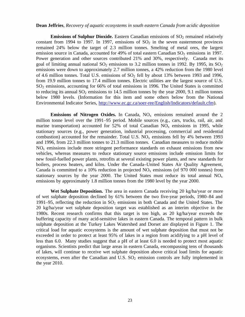
Figure 3. Time series histograms for Ca measurements in George Lake in Killarney Park. The horizontal line is thepre-industrial Ca concentration inferred from diatom fossils in the sediment.

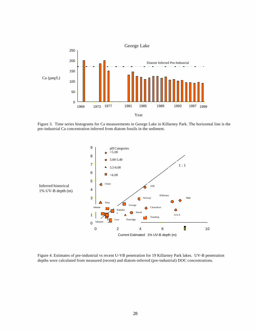
Figure 4. Estimates of pre-industrial vs recent U-VB penetration for 19 Killarney Park lakes. UV-B penetrationdepths were calculated from measured (recent) and diatom-inferred (pre-industrial) DOC concentrations.

0

50

100

150

200

250

1969 1973 1977 1981 1985 1989 1993 1997 1999

Diatom Inferred Pre-Industrial

George Lake

Year

Ca (µeq/L)

Inferred historical1% UV-B depth (m)

0

1

2

3

4

5

6

7

8

9

0 2 4 6 8 10

Current Estimated 1% UV-B depth (m)

Low

Kakakise

Killarney

Chain

pH Categories<5.00

5.00-5.49

5.5-6.00

>6.00

Terry

Johnnie

Ishmael

George

Partridge

David

Norway

Add

Clearsilver

Teardrop

Nelie

O.S.A.

1 : 1

29

Norman Yan, Biological effects of acid deposition

York University, Toronto, Ontario

The partnership between York University and the Ministry of the Environment has twoobjectives:

(1) to quantify long-term changes in the zooplankton of inland lakes in Ontario in response tosingle and multiple stresses: acidity, climatic change, UVR, metals, and non-indigenousspecies,

(2) to identify the factors that regulate recovery of zooplankton from historical damage.

As an example of a long-term change, consider the decline in the number of Cladoceranspecies per standard summer count in Harp Lake (Figure 1). It has decreased sharply in the1990s following the invasion of a new invertebrate predator, the spiny water flea, Bythotrephes.

Figure 1. Reductions in water flea species in Harp Lake

Various projects are currently undertaken in this partnership:(1) Impacts of invaders – with Joelle Young, Stephanie Bordeaux, John Drake, Hugh MacIsaac,

Gary Sprules, Headwaters Inc.(2) Impacts of climatic change – with Jim Rusak, Shelley Arnott, Keith Somers(3) Impacts of UVR – with Anurani Persaud, Mike Arts(4) Impact of falling Ca concentration – with Adam Jeziorski(5) Regulators of recovery from acidification – with Bill Keller, Peter Dillon, Keith Somers, and

Carrie Holt

This presentation focused on Carrie Holt’s MSc research project, Damage and Recovery ofZooplankton Communities in Acidified Lakes of south-central Ontario. This research had twoobjectives:

1980 1985 1990 1995 20001

2

3

4

5

6

7

8

# of

Cla

doce

ran

spec

ies

(with

SE

)

pe

r st

an

da

rd s

um

me

r co

un

t

Year

30

(1) To determine an un-counfounded, zooplankton community based pH endpoint for criticalload models of acidification in south-central Ontario by objective means,

(2) To identify if increases in lake pH’s to above this threshold have resulted in the recovery ofhistorically damaged zooplankton communities.

The first objective was achieved by:(a) identifying if spatial and morphometric confounding existsMorphometric confounding has been previously shown (Yan et al. 1996) to be a function of lakepH and lake area. Factors such as latitude, longitude3, and mean depth were identified as spatialand morphometric factors for species richness (multiple regression, r2 = 0.36). For speciesabundances, latitude, longitude, and log(lake volume) were identified (CCA, variance explained= 36%) to be important.(b) removing this source of variability from total zooplankton varianceSpecies richness = –0.4 (latitude) – 0.1 (longitude)3 + 0.4 (mean depth) + 177 (1)Species abundance = F (latitude, longitude3, log volume) (2)(c) modelling changes in zooplankton community along pH/alkalinity gradientsThe zooplankton community change along an acidity gradient was modelled using a linearmodel (ordinary least squares) and a step function model (regression tree analysis).(d) identifying a threshold of community changeComparisons were made between “corrected” and “uncorrected” models, species richness andabundance models, and between pH and alkalinity models

The second objective was achieved by looking at examples of biological recoverylimited to individual lakes, experimentally manipulated lakes and regional studies. Data fromKillarney Park lakes on zooplankton and water chemistry samples collected between 1971–1973, 1990 and 2000 showed water quality improvements reflected in increases in pH andspecies abundance for some lakes. Lakes which have increased in pH to >6 have recovered,while those which have not increased in pH to >6 have shown some recovery in speciesabundance (Figure 2). Zooplankton species have shown various responses to recovery to a statetypical of neutral lakes (Figure 3).

This research identified a community based biological endpoint for critical load modelsof acidification in south-central Ontario to be a pH of 6. Studies on various individual lakes,experimentally manipulated lakes and regional lakes indicated that recovery to community typestypical of neutral lakes has occurred in some lakes. Many lakes however, are still acidic andtheir recovery may be limited by habitat quality, biotic interactions or dispersal barriers.

pH alk (µµeq/L)

uncorrected abundances 5.98 17.8

richness 5.98 17.8

geographically abundances 5.98 17.8corrected richness 6.07 17.8

morphometrically abundances 5.98 17.8corrected richness 6.07 32.6

31

Figure 2. Recovery to a state typical of neutral lakes

Figure 3. Species abundance

-0.1

0

0.1

0.2

0.3

1971-3 2000

mea

n C

A 1

(p=0.07) (p>0.2)

lakes where pHincreased to >6(n=9)

unacidified lakes

(n=7)

Leptodiaptomus minutus

0

0.4

0.8

1.2

1972 1990 2000

Daphniacatawba

0.2

0.204

0.208

0.212

0.216

0.22

1972 1990 2000

Diaphanosoma spp.

0

0.2

0.4

0.6

0.8

1

1972 1990 2000

Sinobosmina spp.

0

0.2

0.4

0.6

0.8

1

1972 1990 2000

Daphnia retrocurva

0

0.1

0.2

0.3

0.4

0.5

0.6

1972 1990 2000

Tropocyclops spp.

0.2

0.25

0.3

0.35

0.4

0.45

1972 1990 2000

32

Keith Somers, Bioassessments: The effects of stressors on streams. Why do (rapid)bioassessments?

Biological assessments, or bioassessments, offer a number of features that complementmore traditional approaches to water-quality assessments. In particular, biological assessmentsusing benthic invertebrates have gained popularity because benthic invertebrates are: (1)abundant in most aquatic habitats; (2) easily collected with inexpensive gear; (3) easilyidentified; (4) not harvested or exploited (i.e., have no special status like some fish species); (5)sedentary, so they are exposed to local conditions; (6) represented by many species withdifferent sensitivities to a wide array of pollutants and different life cycles ranging from weeksto years; (7) sensitive to both spills and long-term (low-level) exposures; (8) integrate the effectsof all pollutants over time; (9) demonstrate pollution effects, not just the presence or amount ofpollutants; and (10), bio-accumulate pollutants that are often present in low concentrations.

Several biological monitoring programs were initiated at Dorset in the late 1980s in acollaboration between the federal and provincial governments known as the Long RangeTransport of Atmospheric Pollutants (LRTAP) Program. The LRTAP Program was designed toassess the anticipated recovery of inland waters associated with reductions in atmosphericpollutant loadings (Shaw et al. 1992). The Dorset programs began in 1988 and evaluatednearshore benthic communities at 5 sites in each of 12 lakes. Each littoral sample was collectedusing a standardized kick-and-sweep protocol. All invertebrates were picked from each sample,and the animals were identified to the lowest practical taxonomic level (i.e., some immatureindividuals could not be identified to species).

The program continued for 5 years with detailed data on benthos and water chemistry.Because the benthic samples were picked in their entirety and then identified through contractsto external taxonomic experts, the approximate turn-around time from sample collection to dataevaluation and reporting was 2 years. By contrast, water chemistry samples were processed andthe data were available for evaluation in 30-50 days. In an effort to complete the biologicalassessments in a more timely and cost-effective manner, rapid bioassessment strategies proposedby the US EPA were adopted. This protocol offered significant savings because only 100animals are removed from a sample and these individuals are identified to the coarse taxonomiclevels of order or family (e.g., see David et al. 1998). As a result, the turn-around time for thebiomonitoring data has been cut from roughly 2 years to one day per lake.

The Dorset LRTAP program continues in its new rapid bioassessment form focusing onthe 9 “A” lakes where water chemistry data are routinely collected. In addition, several basicassumptions underlying the rapid bioassessment protocol have been evaluated. Theseassumptions include: (1) is 100 animals enough to adequately characterize the benthiccommunity at a given site?; (2) is order or family-level taxonomy sufficient?; and (3), does therapid bioassessment protocol provide enough resolution to detect impairment?

To evaluate whether a count of 100 animals is enough, 100, 200 and 300 animals werecounted from 5 sites in each of 5 lakes (see Somers et al. 1998). A variety of summary indiceswere calculated using the resultant data, and one-way ANOVAs were used to compare the 5lakes based on each index. Although results varied among indices, the general finding was thatcounts of more than 100 animals provided only minor gains in distinguishing the 5 lakes (seeTable 1). Thus, 100 animals is enough for our purposes.

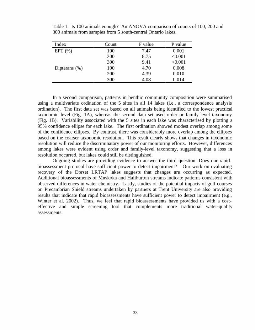
33

Table 1. Is 100 animals enough? An ANOVA comparison of counts of 100, 200 and300 animals from samples from 5 south-central Ontario lakes.

Index Count F value P valueEPT (%) 100 7.47 0.001

200 8.75 <0.001300 9.41 <0.001

Dipterans (%) 100 4.70 0.008200 4.39 0.010300 4.08 0.014

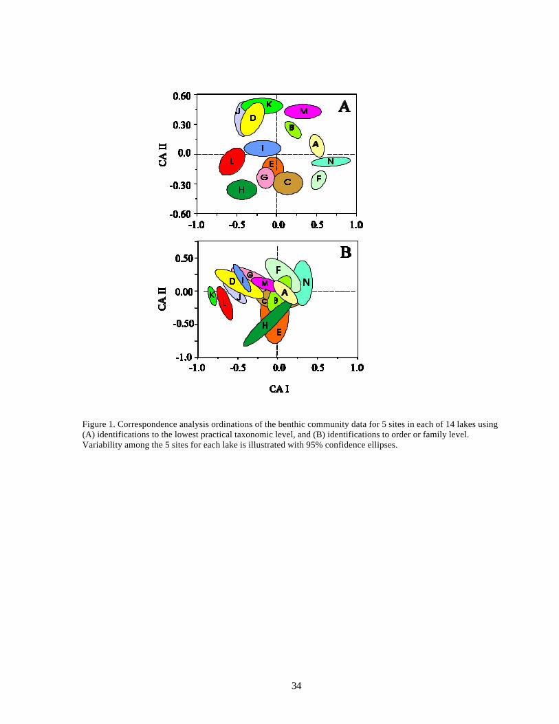
In a second comparison, patterns in benthic community composition were summarisedusing a multivariate ordination of the 5 sites in all 14 lakes (i.e., a correspondence analysisordination). The first data set was based on all animals being identified to the lowest practicaltaxonomic level (Fig. 1A), whereas the second data set used order or family-level taxonomy(Fig. 1B). Variability associated with the 5 sites in each lake was characterised by plotting a95% confidence ellipse for each lake. The first ordination showed modest overlap among someof the confidence ellipses. By contrast, there was considerably more overlap among the ellipsesbased on the coarser taxonomic resolution. This result clearly shows that changes in taxonomicresolution will reduce the discriminatory power of our monitoring efforts. However, differencesamong lakes were evident using order and family-level taxonomy, suggesting that a loss inresolution occurred, but lakes could still be distinguished.

Ongoing studies are providing evidence to answer the third question: Does our rapid-bioassessment protocol have sufficient power to detect impairment? Our work on evaluatingrecovery of the Dorset LRTAP lakes suggests that changes are occurring as expected.Additional bioassessments of Muskoka and Haliburton streams indicate patterns consistent withobserved differences in water chemistry. Lastly, studies of the potential impacts of golf courseson Precambrian Shield streams undertaken by partners at Trent University are also providingresults that indicate that rapid bioassessments have sufficient power to detect impairment (e.g.,Winter et al. 2002). Thus, we feel that rapid bioassessments have provided us with a cost-effective and simple screening tool that complements more traditional water-qualityassessments.

34

Figure 1. Correspondence analysis ordinations of the benthic community data for 5 sites in each of 14 lakes using(A) identifications to the lowest practical taxonomic level, and (B) identifications to order or family level.Variability among the 5 sites for each lake is illustrated with 95% confidence ellipses.

35

Julie Schulenburg, Master Thesis Proposal: Determining the impacts of golf courseconstruction and operation on the benthic macroinvertebrate communities in streams on thePrecambrian Shield

This research is testing the hypothesis that construction and operation of golf courseslocated on the Precambrian Shield alter benthic macroinvertebrate community structure instreams. Potential disturbances due to golf course development are clear cutting using machineryand/or herbicides, the addition of millions of tons of sand, the introduction of non-indigenousgrass and plant species, and the application of fertilizers and pesticides for maintenance. Basedon the hypothesis above, it is expected: (1) a decrease in the number of macroinvertebrates thatare intolerant to organic pollutants during the study period, (2) an increase in the number ofmacroinvertebrates that are tolerant to organic pollutants, and (3) a reduction in the taxonomicrichness. The purpose of this study is to evaluate changes in benthic macroinvertebratecommunity structure downstream from golf courses using the rapid bioassessment method. Thestudy area is located in the District of Muskoka on the south edge of the Precambrian Shield.Thirty-eight sampling sites where chosen for study, nineteen reference sites located in arelatively pristine forest and nineteen test sites located downstream or on a golf course.

Methodology involved sampling of water chemistry, the rapid bioassessment ofmacroinvertebrates, and substrate survey for three years between 1999 and 2001 during spring,summer and fall. The River Bank Quality Index (RBQI) was calculated from a field survey ofthe riparian vegetation buffer strip in summer of 2001. The collection of data on streamdischarge, air temperature and precipitation was also required for the study. Stream discharge,air temperature and precipitation was recorded regularly by MOE Dorset technicians as part oftheir regular data collection. Stream discharge was extrapolated for some test sites fromneighbouring catchments. Extrapolated stream flow is calculated by dividing stream catchmentarea at the reference sites into measured stream flow, then multiplying by the catchment area ofthe test site. This extrapolated value of the test site was compared to actual stream flow that wasmeasured in the field at random times.

Various statistical analyses were applied to the data to explain how water chemistry,substrate, riparian vegetation, stream discharge, air temperature and precipitation play a role intaxa differences. Two approaches were undertaken for the statistical analyses. For the reference-condition approach, regional reference conditions were defined by using the Jaccard distancemeasure to classify the reference sites using taxa indices. Multidimensional Scaling (MDS)was applied to reference sites using the similarity matrices, and the Discriminant FunctionalAnalysis (DFA) was applied to find physical stream attributes that best discriminate between thereference groups and to assign each site to an appropriate reference group. The DFA test wasalso applied to determine if the taxa indices of the test group were significantly different fromthe reference sites. The second approach (Before/After Impact) was applied using Kolmogorov-Smirnov goodness of fit test to golf course (test) sites to determine if there was a significantdifference in taxa frequencies between years 1999, 2000 and 2001. Reasons for thesedifferences were explored by examining the substrate, water chemistry, buffer strip vegetation,stream discharge and weather patterns.

36

Isabelle Lavoie, Doctoral Thesis Proposal: Diatoms as a biological indicator of water qualityin streams of Ontario and Quebec

Water quality degradation in streams affected by anthropogenic activities is generallydue to eutrophication and high organic and mineral inputs. Physical and chemical measurementsused in water quality monitoring are an important guide to environmental change, but they areonly representative of conditions found at the instant of sampling and do not provideinformation about the effects of these changes on biological communities. The use of abioindicator provides an integrated measurement of water quality as experienced by the aquaticbiota, and therefore offers a useful addition to water quality monitoring strategies. In manyEuropean countries, water quality monitoring is achieved using biological indices based onbenthic diatoms (microscopic algae fixed on substrates). Diatoms are particularly sensitive tochanges in nutrient concentrations (principally phosphorus and nitrogen) and to organic andmineral charges. Some diatom species are very sensitive and do not tolerate pollution whileother species are very tolerant and will dominate in eutrophic ecosystems. Diatoms have a fastgrowth rate and respond to a change in environmental conditions within a short period of time(2-4 weeks). There are many thousands species of benthic diatoms, but about 700 species arecommonly found in rivers. European indices are built taking into account the relative abundanceof each species, their sensitivity, and their indicator value (species that live in all type ofecosystems have less weight in the index calculation). Diatom indices reflect changes incommunity structure as a result of disturbance in the system. Many studies carried out in Canadashow the potential of diatom communities as an indicator of water quality. However, there areno diatom indices currently used in water quality monitoring programs in Canada.

The general goal of the project is to apply (and adapt if necessary) the existing Europeanindices on diatom communities in Canadian streams and rivers to provide a tool for biologicalwater quality monitoring. This overall goal is based on the assumption that benthic diatomcommunity structure is a good indicator of water quality in Canada. This primary hypothesiswill be evaluated by analysing the relationships between diatom community structure andenvironmental variables. The existing European indices will then be tested, assuming they are anaccurate indicator of water quality in Canadian streams and rivers. To verify this hypothesis,multivariate analysis will be conducted to analyse the relationship between European diatomindices and environmental variables. It is essential to test the European indices in order to verifyif the species ecological preferences in Europe and Canada are similar.

37

Andrew Paterson, Paleolimnological Studies: Acid deposition/ Climate Change

Long-term monitoring data form an integral part of lake management programs. Theexisting data sets in Ontario have been important in understanding the effects of majorenvironmental stresses (e.g., acid deposition) on water quality of lakes, however these data setsare often too short in duration to determine the conditions prior to the onset of disturbances.Paleolimnology allows an extension of the monitoring information back in time and thus worksin compliment with the existing data. There are at least three main advantages to usingpaleolimnological data: (1) it can be used to understand background/baseline conditions, and cangive estimates of natural variability, (2) it can give some indication of the timing/rate of change,(3) it provides a consistent methodology over very long time periods.

Paleolimnological data can be divided into three broad categories, calibration data, top-bottom analysis and core work. The calibration data or training sets consist of biological remainsfrom the surface sediment of lakes within a region (i.e. top ½ to 1cm), and existing present-dayphysical and chemical variables. Using a variety of modeling techniques these data can be usedto compute models for reconstructing environmental variables back in time (Figure 1). Thegeographic location of calibration data is important. In Ontario, there are more than 400 lakesfor which calibration data exist. This data allows moving from the modeling stage to askinglong-term questions regarding environmental changes in lakes. The biological information forseveral key indicators is useful for constructing Paleolimnological models. Indicators such asdiatoms and chrysophytes are used to reconstruct a variety of environmental variables, includinglake water pH, TP, TN, conductivity and DOC. The remains of chironomid larvae have beenused in Ontario to reconstruct long-term trends in hypolimnetic oxygen concentrations. There isalso the potential to extract information from other organisms that preserve in lake sediments,including cladoceran remains. Top-bottom analysis data includes top-bottom samples based on apoint estimate of background or pre-disturbance conditions and core data involves looking atcontinuous trends in water quality through time (Figure 2). Currently, the primary objective ofthe MOEE at Dorset is to centralise existing paleolimnological data in Ontario into an Access-based database.

A number of questions can be explored using the paleolimnological data:

(1) Has water transparency (DOC) changed since the pre-industrial times? Over the lastmillennia? Are these changes related to acid deposition and climate? Currently,models using diatoms are used for reconstructing long-term trends in DOC. In theSudbury region, these models have been examined to estimate long-term changes inUV-B exposure

(2) Are long-term changes in water transparency linked to changes in fisheries habitat(related to hypolimnetic oxygen concentrations)? The remains of chironomid larvaehave been used as paleo-indicators of hypolimnetic oxygen concentrations. A goodrelationship was found between the chironomid assemblages and oxygen, as taxahave different levels of tolerance to low oxygen concentrations

(3) What is the importance of acid deposition relative to climate (and other factors) ininfluencing biological assemblages? Are the interactive effects of acid deposition andclimate important? Long-term paleolimnological data allows to quantify therelationship between key groups of stressors unexplained so far (e.g. acid depositionor climate) and biological changes. The unique variance explained can be estimatedusing a technique called variance partitioning analysis. Furthermore, the varianceexplained by combinations of variables, such as acid deposition and climate can beestimated.

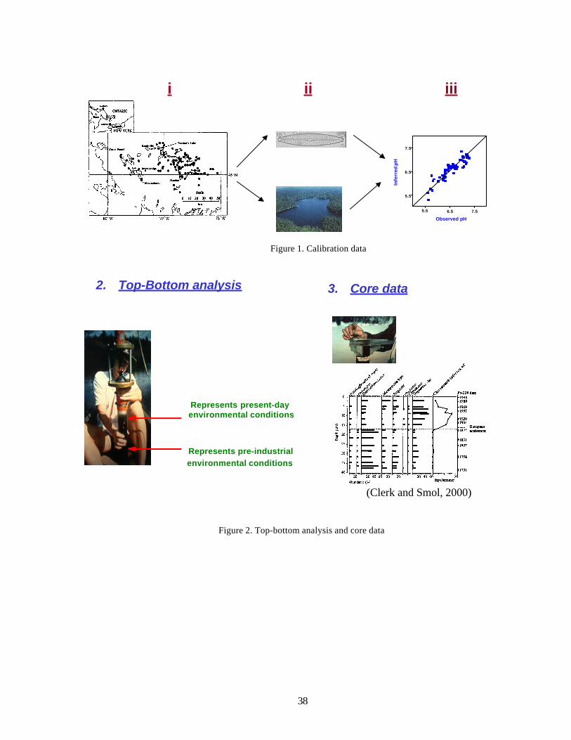
38

Figure 1. Calibration data

(Clerk and Smol, 2000)

Figure 2. Top-bottom analysis and core data

5.5 6.5 7.5

5.5

6.5

7.5

Observed pH

Infe

rre

d p

H

i ii iii

2. Top-Bottom analysis

Represents present-day environmental conditions

Represents pre-industrial

environmental conditions

3. Core data

39

Lewis Molot, Photo-Oxidation of Humic DOC in Northern Lakes

Research on dissolved organic carbon (DOC) in lakes is important because it affects lightpenetration, therefore affecting heat budgets, epilimnetic mixing depth and photosynthesis. Italso provides “sunscreen protection” against UV penetration in lakes. DOC forms complexeswith metals of varying affinities, and reduces losses of biologically necessary, relativelyinsoluble metals such as iron. The objectives of the presented research are: (1) to measure andmodel DOC fluxes into and out of Dorset study lakes, (2) to measure and model DOC fluxes tosediments (as particulate organic C, (POC)) and the atmosphere (as CO2), (3) identify primarycontrols of in-lake DOC processing. Three approaches are undertaken: (1) regression modellingof long-term mean of DOC export from headwater stream catchments, (2) steady-state massbalance modelling of long-term mean DOC losses in lakes with loss partitioned betweensediments and the atmosphere, and (3) experimentally examined short-term DOC lossmechanisms in lakes, with focus on the roles of UV and iron. The presentation focused on themechanisms, and the role of UV and iron for DOC loss in lakes.

Regression modelling shows that DOC export from headwater catchments is stronglycorrelated with the proportion of peatlands. Mass balance modelling also yields some importantinformation: net loss of carbon to the atmosphere (i.e. evasion exceeds invasion at thelake/atmosphere surface) was suggested, indicating that catchments are important sources of C,mostly as DOC, wetlands are a major source of lake carbon, acidity affects partitioning ofretained carbon between sediments and atmosphere, and approximately 120 Pg C hasaccumulated in boreal lake sediments globally since the last glaciation.

The steady state mass balance modelling in lakes is based on the following equations:

Input = Output (1)Load = (Discharge) + (Sediment + Atmospheric Losses) (2)

Applied to DOC and assuming 1st order kinetics,Load = q [DOC] + í[DOC] (3)[DOC] = Load / (q + í)Where: q is the areal water discharge rate (m/yr), í is the mass transfer coefficient (m/yr)

(í combines atmospheric and sediment losses and it is empirically determined). For sevenDorset lakes, mass transfer coefficients were determined to be 0.9 ± 0.1 and 2.8 ± 0.8 tosediments and atmosphere, respectively at < 20: eq/l lake alkalinity and 1.9 ± 0.5 and 1.0 ± 0.9to sediments and atmosphere, respectively at > 20: eq/l lake alkalinity.

In DOC photo-oxidation experiments, the loss of DOC was measured using the equation:

d[DOC] / dt = - ki[DOC] (4)

Where k is corrected for dark loss and ki is normalized for variation in broad UV band.Loss of organic matter in lakes occurs by (1) direct photolysis and (2) indirect photolysis

where sunlight has a direct effect on NO3-, and Fe3+, ultimately resulting in the production of

O2-, H2O2, OH-, CO3

- and OH-. The reduction of Fe3+ to Fe2+ under the effect of UV and theoxidation of Fe2+ with H2O2 (hydrogen peroxide) at low pH leads to enhanced production ofhydroxyl radical (OH-). Photo-production of hydroxyl radicals is also enhanced via nitrate (peak301 nm) and nitrite (peak 354 nm), however this pathway is not pH sensitive.

Titration experiments indicated that the highest oxidation and loss of DOC under theeffect of UV light occurs at the lowest pH of 4. The addition of sodium fluoride (NaF) promoted

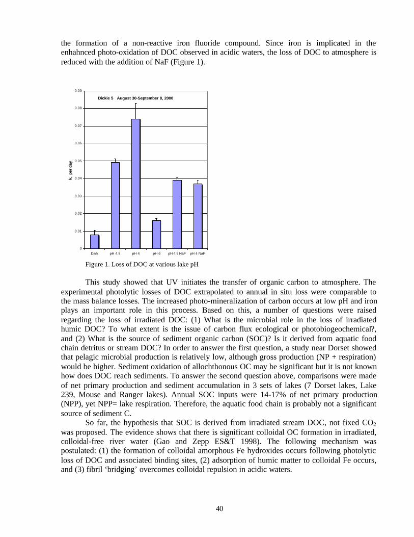
40

the formation of a non-reactive iron fluoride compound. Since iron is implicated in theenhahnced photo-oxidation of DOC observed in acidic waters, the loss of DOC to atmosphere isreduced with the addition of NaF (Figure 1).

Figure 1. Loss of DOC at various lake pH

This study showed that UV initiates the transfer of organic carbon to atmosphere. Theexperimental photolytic losses of DOC extrapolated to annual in situ loss were comparable tothe mass balance losses. The increased photo-mineralization of carbon occurs at low pH and ironplays an important role in this process. Based on this, a number of questions were raisedregarding the loss of irradiated DOC: (1) What is the microbial role in the loss of irradiatedhumic DOC? To what extent is the issue of carbon flux ecological or photobiogeochemical?,and (2) What is the source of sediment organic carbon (SOC)? Is it derived from aquatic foodchain detritus or stream DOC? In order to answer the first question, a study near Dorset showedthat pelagic microbial production is relatively low, although gross production (NP + respiration)would be higher. Sediment oxidation of allochthonous OC may be significant but it is not knownhow does DOC reach sediments. To answer the second question above, comparisons were madeof net primary production and sediment accumulation in 3 sets of lakes (7 Dorset lakes, Lake239, Mouse and Ranger lakes). Annual SOC inputs were 14-17% of net primary production(NPP), yet NPP= lake respiration. Therefore, the aquatic food chain is probably not a significantsource of sediment C.

So far, the hypothesis that SOC is derived from irradiated stream DOC, not fixed CO2

was proposed. The evidence shows that there is significant colloidal OC formation in irradiated,colloidal-free river water (Gao and Zepp ES&T 1998). The following mechanism waspostulated: (1) the formation of colloidal amorphous Fe hydroxides occurs following photolyticloss of DOC and associated binding sites, (2) adsorption of humic matter to colloidal Fe occurs,and (3) fibril ‘bridging’ overcomes colloidal repulsion in acidic waters.

Dickie 5 August 30-September 8, 2000

0

0.01

0.02

0.03

0.04

0.05

0.06

0.07

0.08

0.09

Dark pH 4.9 pH 4 pH 6 pH 4.9 NaF pH 4 NaF

k, p

er d

ay

41

Dolly Kothawala, Master Thesis Project: Spatial and temporal patterns of dissolved organiccarbon (DOC) molecular size distribution by high performance size exclusion chromatography(HPSEC)

Dissolved organic carbon (DOC) is a heterogenous mixture of compounds ubiquitous innature. Humic substances are the main ingredients, which are by definition resistant to furtherdecay by microbial organisms. Some of the roles of DOC in surface waters are (1) to control thelevel of trace metal bioavailability in aquatic environments, (2) to absorb harmful UV radiation,thus offering protection to aquatic biota and (3) to enhance the buffering capacity of water byaccepting/donating hydrogen ions (H+). The molecular size/weight of DOC is a very usefulindicator of its chemical properties (e.g. molecular weight for assessing the quality of DOC),which requires a technique with high resolution in order to detect subtle changes in themolecular weight (MW) distribution. The objectives of this research are (1) to establish amethod capable of resolving subtle differences in size distribution for DOC in stream waters,and (2) utilising this method, to determine spatial and temporal patterns of DOC size distributionwithin a stream.

The study site was chosen at the Harp 4 sub-catchment located in the Harp Lakecatchment, on the Precambrian Shield. Harp 4 sub-catchment encompasses a headwater swampand a series of beaver ponds. For the purpose of this study, the stream was divided into‘upstream’, ‘beaver ponds’ and ‘downstream’ sites (Figure 1). Temporal trends (May-November) for DOC concentrations showed lower values between July and August for theupstream and downstream sites. The lowest temporal variability in DOC concentrations wasmeasured at the Beaver Ponds, with values ranging between 11-15 mg/L DOC and the highestvariability was measured at the upstream sites with DOC concentrations ranging between 10-45mg/L.

The high performance size exclusion chromatography (HPSEC) method sievesmolecules based on size. The size fractions were chosen as follows: large (> 5000 Da), medium(5000 – 1500 Da) and small (< 1500 Da). The absorption at 254 nm (AU) was highest for theupstream sites. Figure 2 shows DOC concentrations at various sites and DOC size. The effectsof summer drought on molecular weight fractions showed that a lower percent abundance ofMW was measured following the drought than prior to the drought. Spatially, a higher MWpercent abundance of molecules passing through large pores was measured at the downstreamsites. Also at downstream sites, a lower MW percent abundance of molecules passing throughmedium and medium-large pores was recorded. The percent abundance of molecules passingthrough small pores was highly variable. A shifting in the size of DOC was observed at theBeaver Ponds.

This research showed that the rate of DOC loss is highly variable and it is based on thenature of DOC. Measuring the DOC loss is useful in identifying the age of DOC spatially. Theoverall decrease in average MW from the headwater swamp downstream to the lake wasapproximately 500 Da. Future research is needed to identify the significance of this change bothbiologically and environmentally. The Beaver Pond caused a significant decrease in the quantityof DOC and it displayed a shifting in the size distribution of DOC. Beaver Ponds may play animportant role in lowered water table scenarios. The HPSEC method may be useful in tracingbiogeochemical pathways of DOC in situ.

42

Figure 1. Spatial DOC concentration for Harp 4 sub-catchment

Figure 2. DOC concentration and DOC size at the study sites

0

1

2

3

4

522-Jun-0119-Jul-0127-Aug-0125-Sep-0105-Oct-01

0

5

10

15

20

0

10

20

30

40

0

5

10

15

BeaverPonds

Hp 4-4 Wetland

Hp 4-4 Wetland

BeaverPonds

BeaverPonds

Large: >5.0 kDa Medium: 2.0 to 1.5 kDa

Medium / Large: 5.0 - 2.0 kDa Small: <1.5 kDa

0

10

20

30

40

50

Site

DO

C C

once

ntra

tion

(mg/

L)

Beaver Ponds

Wetland/Beaver PondHeadwater Swamp

UPSTREAM

DOWNSTREAM

BeaverPonds

43

APPENDIX AReferences

Aherne, J., Posch, M., Rusmir, C., Dillon, P.J. and A. Henriksen. 2002. Critical load of acidityto surface waters in south-central Ontario, Canada. II. Application of the First-order AcidityBalance (FAB) model. NIVA, Oslo, Norway, 30 pp.

Arnott, S. E., Yan, N., Keller, W. and K. Nicholls. 2001. The influence of drought-induced acidification on the recovery of plankton in Swan Lake. Ecological Applications 11:747-763.

Beall, F.D., Semkin, R.G. and D.S. Jeffries. 2001. Trends in the output of first-orderbasins at Turkey Lakes Watershed, 1982-96. Ecosystems 6(4): 514-526.

David, S.M., Somers K.M., Reid, R.A., Hall, R.J. and R.E. Girard. 1998. Samplingprotocols for the rapid bioassessment of streams and lakes using benthic macroinvertebrates. 2ndedition. Dorset Environmental Science Centre, Ontario Ministry of the Environment, Dorset,ON. ISBN: 0-7778-7378-8.

Dillon, P.J., Nicholls, K.H., Scheider, W.A.,Yan, N.D and D.S. Jeffries. 1994. Lakeshorecapacity study: Part I – Test of effects of shoreline development on the trophic status of lakes.Lake Reserv. Manage. 8: 121-129.

Dillon, P.J., Molot, L.A. and M. Futter. 1997. The effect of El Nino-related drought onthe recovery of acidified lakes. Environ. Monit. Assess. 46: 105-111.

Gunn, J. M. and W. Keller. 1990. Biological recovery of an acid lake after reductions inindustrial emissions of sulphur. Nature 345: 431-433.

Gunn, J. M., Snucins, E., Yan, N and M. Arts. 2001. Use of water clarity to monitor theeffects of climate change and other stressors on oligotrophic lakes. Environmental Monitoring and Assessment 67: 69-88.

Henriksen, A. and P.J. Dillon. 2001. Critical Load of Acidity to Surface Waters in South-Central Ontario, Canada. I. Application of the Steady-State Water Chemistry (SSWC)Model. NIVA, Oslo, Norway, 31 pp.

Henriksen, A. and Posch, M. 2001. Steady-State Models for calculating critical loads ofacidity for surface waters. Water, Air and Soil Pollution: Focus 1: 375–398.

Jeffries, D.S., Semkin, R.G., Beall, F.D. and J. Franklyn. 2002. Temporal trends in waterchemistry in the Turkey Lakes Watershed, Ontario, Canada, 1982-1999. Wat. Air SoilPollut.: Focus 2: 5-22.

Keller, W., Pitblado, J.R. and J. Carbone. 1992. Chemical responses of lakes in theSudbury, Ontario area to reduced smelter emissions, 1981-1989. Canadian Journal ofFisheries and Aquatic Sciences 49 (Supplement 1): 25-32.

44

Keller, W., Gunn, J.M. and N. D. Yan. 1999. Acid rain - perspectives on lake recovery.Journal of Aquatic Ecosystem Health and Recovery 6: 207-216.

Keller, W., Dixit, S.S. and J. Heneberry. 2001. Calcium declines in northeastern Ontariolakes. Canadian Journal of Fisheries and Aquatic Sciences 58: 2011-2020.

Keller, W., Heneberry, J., Dixit, S. and R. Vet. (under review). Atmospheric depositionand the chemical recovery of Killarney, Ontario, lakes. Ambio.

LaZerte, B.D. and P.J. Dillon. 1984. Relative importance of anthropogenic versus naturalsources of acidity in lakes and streams of central Ontario. Can. J. Fish. Aquat. Sci. 41:1664-1677.

Neary, B. P., Dillon, P.J., Munro, J.R. and B. J. Clark. 1990. The Acidification of OntarioLakes: an Assessment of Their Sensitivity and Current Status With Respect to BiologicalDamage. Tech. Rep. Ontario Ministry of Environment and Energy, Dorset, Ontario,Canada, 171 pp.

Nilsson, J. and Grennfelt, P. (eds) 1988. Critical Loads for Sulfur and Nitrogen. NordicCouncil of Ministers, Miljørapport 1988:15, 418 pp.

Rusak, J.A., Yan, N.D., Somers, K.M. and D.J. McQueen. 1999. The temporal coherenceof zooplankton population abundances in neighbouring north-temperate lakes. Am. Nat.153: 46-58.

Schiff, S., Aravena, R., Mewhinney, E., Elgood, R., Warner, B., Dillon, P. and S.Trumbore.1998. Precambrian shield wetlands: hydrologic control of the sources and export ofdissolved organic matter. Climatic Change 40: 167-188.

Schiff, S.L., Aravena, R., Trumbore, S.E., Hinton, M.J., Elgwood, R. and P.J. Dillon. 1997.Export of DOC from forested catchments on the Precambrian Shield of Central Ontario: Cluesfrom 13C and 14C.

Schiff, S.L., Aravena, R., Trumbore, S.E. and P.J. Dillon. 1990. Dissolved organic carboncycling in forested watersheds: a carbon isotope approach. Water Resources Res. 26: 2949-2957.

Schindler, D.W. 2001. The cumulative effects of climate warming and other humanstresses on Canadian freshwaters in the new millennium. Can. J. Fish. Aquat. Sci. 58: 18-29.

Shaw, M.A., Geiling, S., Barbour, S., Davies, I.J., Hamilton, E.A., Kemp, A., Reid, R.,Ryan, M., Watson, N. and W. White. 1992. The Department of Fisheries and Oceansnational LRTAP biomonitoring programme: site locations, physical and chemicalcharacteristics. Can. Tech. Rep. Fish. Aquat. Sci. 1875: 87 pp.

Snucins, E. and J. Gunn. 2000. Interannual variation in the thermal structure of clear andcolored lakes. Limnology and Oceanography. 45: 1639-1646.

45

Somers, K.M., Reid, R. A., and S.M. David. 1998. Rapid biological assessments: howmany animals are enough? J. N. Am. Benthol. Soc. 17: 348-358.

Winter, J.G., Somers, K.M., Dillon, P.J., Paterson, C. and R.A. Reid. 2002. Impacts ofgolf courses on macroinvertebrate community structure in Precambrian Shield streams. J.Environ. Qual. (in press).

Yan, N. D., Keller, W., Scully, N.M., Lean, D.R.S. and P. J. Dillon. 1996. Increased UV-B penetration in a lake owing to drought-induced acidification. Nature 381: 141-143.

46

APPENDIX BList of addresses

Julian Aherne, Environmental and Resource Science Program, Trent University, Peterborough,ON, K9J 7B8, julian.aherne@ucd.ie

Shaun Watmough, Environmental and Resource Science Program, Trent University,Peterborough, ON, K9J 7B8, swatmough@trentu.ca,

Keith Somers, Ontario Ministry of the Environment and Energy, Dorset Environmental ScienceCentre, PO Box 39, Dorset, ON, P0A 1E0, Keith.somers@ene.gov.on.ca

Jim Buttle, Environmental and Resource Science Program, Trent University, Peterborough, ON, K9J 7B8, jbuttle@trentu.ca

Catherine Eimers, Department of Earth Sciences, University of Waterloo, Waterloo, ON, N2L3G1, ceimers@trentu.ca

Peter Dillon, Environmental and Resource Science Program, Trent University, Peterborough, ON, K9J 7B8, pdillon@trentu.ca

Sherry Schiff, Department of Earth Sciences, University of Waterloo, Waterloo, ON, N2L 3G1, sschiff@sciborg.uwaterloo.ca

Dean S. Jeffries, Environment Canada, National Water Research Institute, P.O. Box 5050,Burlington, ON, L7R 4A6, Dean.Jeffries@ec.gc.ca

Bill Keller, Ontario Ministry of the Environment and Energy, Sudbury, ON, P3E 2C6,bkeller@vianet.ca

Norman Yan, Department of Biology, York University, Toronto, ON, M3J 1P3cnturybb@muskoka.com

Julie Schulenburg, Watershed Ecosystems, Trent University, Peterborough, ON, K9J 7B8,jschuleburg@trentu.ca

Isabelle Lavoie, Watershed Ecosystems, Trent University, Peterborough, ON, K9J 7B,Ilavoie@trentu.ca

Andrew Paterson, Ontario Ministry of the Environment and Energy, Dorset Environmental Science Centre, PO Box 39, Dorset, ON, P0A 1E0, Andrew.Paterson@ene.gov.on.ca

Lewis Molot, Department of Biology, York University, Toronto, ON, M3J 1P3, lmolot@YorkU.CA

Dolly Kothawala, Watershed Ecosystems, Trent University, Peterborough, ON, K9J 7B8,dkothawala@trentu.ca

47