operator representation of an networks of pdes modeling a

Prirodoslovno-matematicki fakultet

Matematicki odsjek

Sveuciliste u Zagrebu

Operator representation of an networks of PDEs modelinga coronary stent

OTIND 2016, Vienna, December 20, 2016

Luka Grubisic, Josip Ivekovic and Josip TambacaDepartment of Mathematics, University of [email protected]

Luka Grubisic 1 / 44

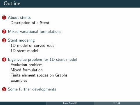
Outline

1 About stentsDescription of a Stent

2 Mixed variational formulations

3 Stent modeling1D model of curved rods1D stent model

4 Eigenvalue problem for 1D stent modelEvolution problemMixed formulationFinite element spaces on GraphsExamples

5 Some further developments

Luka Grubisic 2 / 44

About stents

• carotid stenosis

• stent: ”solution” of the problem

About stents Luka Grubisic 3 / 44

Stent properties

• A network of cylindrical tubes (made by laser cuts)

• Typically: 316L stainless steel, but also cobalt, chrome and nickel.

• expanded on the place of stenosis (balloon expandable is dominant(99%) over self-expanding)

• properties depend onI complex geometry of a stent,I mechanical properties of material.

• metaltheory of elasticity

• start from a conservation lawconstrained evolution problems


Plan

Mixed variational formulations are good for analyzing systems with

constraints.Modal analysis gives first information on time evolution.

Mixed eigenvalue problems

Let us review two canonical approaches to mixed eigenvalue problems


Type I

Dirichlet eigenvalue problem

−4u = λu

u ∈ H = H10

• No finite accumulation points

• eigenfunctions make an orthonormal system for H.

A mixed formulation reads

H =

[I −Div

Grad 0

], M =

[0−I

].

Modeli Luka Grubisic 8 / 44

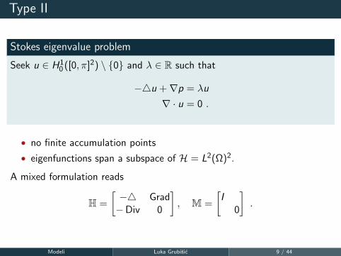
Type II

Stokes eigenvalue problem

Seek u ∈ H10 ([0, π]2) \ 0 and λ ∈ R such that

−4u +∇p = λu

∇ · u = 0 .

• no finite accumulation points

• eigenfunctions span a subspace of H = L2(Ω)2.

A mixed formulation reads

H =

[−4 Grad−Div 0

], M =

[I

0

].


Some pictures

IsoValue-35.5992-30.5136-27.1232-23.7328-20.3424-16.952-13.5616-10.1712-6.7808-3.3904-1.68677e-0083.39046.780810.171213.561616.95220.342423.732827.123235.5992

Vec Value00.09003510.180070.2701050.3601410.4501760.5402110.6302460.7202810.8103160.9003510.9903861.080421.170461.260491.350531.440561.53061.620631.71067

Eigen Vector 0 valeur =52.3471

• For Type I take P1–P0

• For Typer II take P2–P1


Quasidefinite block operator matrices – form aproach

• Split the sesquilinear form

h(u, v) = k(u1, v1) + b(u1, v2) + b(v1, u2),

as

h = k + b '(K B∗

B 0

).

• representation theorems self-adjoint operators

I Ker(h) = (Ker(K ) ∩ Ker(B))⊕ Ker(B ′)I higher order Sobolev spaces and interpolation results?I indefinite Cholesky on the level of block operator matrices e.g.

Grubisic, Kostrykin, Makarov, Veselic 2013

• This is indeed a special structure, recall the talk of C. Tretter or A.Motovilov.

With this we have access to spectral calculus to study constrainedproblems!


Representation theorems for quasidefinite matrices

For h we obtain a representation theorem

h(u, v) = (Hu, v)H

where

H =

[K B∗

B 0

]denotes the operator defined by h with

Dom(H) = (Dom(K ) ∩ Dom(B))⊕ Dom(B∗)

If K is invertible then

H =

[I 0

BK−1 I

] [K−BK−1B∗

] [I K−1B∗

0 I

].

Has a flavor of a second representation theorem if the domain stability

condition holds.Modeli Luka Grubisic 12 / 44

Similarity transformations

Since

H =

[I 0

BK−1 I

] [K−BK−1B∗

] [I K−1B∗

0 I

].

and [I 0

BK−1 I

]−1

=

[I 0

−BK−1 I

]if follows [

K−BK−1B∗

] [uv

]= λ

[0−M

] [uv

].

and soBK−1B∗v = λMv

is an equivalent eigenvalue problem.


Similarity transformations

For Type II there are various equivalent reformulations (should K be

singular) like [K + B∗B B∗

B 0

] [up

]= λ

[M

0

] [up

].

since [I B∗

0 I

] [K B∗

B 0

]=

[K + B∗B B∗

B 0

]and so M stays unchanged.

Recall

H−1 =

[K−1 − K−1B∗(BK−1B∗)−1BK−1 K−1B∗(BK−1B∗)−1

(BK−1B∗)−1BK−1 −(BK−1B∗)−1

].


Finally ...

[up

]= λ

[(K−1 − K−1B∗(BK−1B∗)−1BK−1)Mu

(BK−1B∗)−1BK−1Mu

].

and so [up

]= λ

[TMuSMu

].

which yields a reduced problem (in Ker(B))

T−1u = λMu .

All finite eigenvalues of the reduced and the full problem coincide.

Infinity is an eigenvalue of the saddle-point problem and it has

associated vectors (cf. Spence et.al.).


Standard variational approach

Define solution operator T : H → Dom(k) and S : H → Dom(B),

k(Tf , uS) + b(Sf , uS) = (f , uS), uS ∈ Dom(k),

b(nS ,Tf ) = 0, nS ∈ Dom(B∗).(2.1)

Require only ellipticity of kS in Ker(B),

Recall Ker(H) = (Ker(K ) ∩Ker(B))⊕Ker(B∗), eg.

Benzi-Liesen-Golub, for matrices Tretter, Veselic and Veselic for operators.When K invertible

T = (K−1 − K−1B∗(BK−1B∗)−1BK−1)

further information cf. Boffi–Brezzi–Marini


Constraint satisfaction and computability

Direct computation yields

BT =

= B(K−1 − K−1B∗(BK−1B∗)−1BK−1)

= BK−1 − BK−1B∗(BK−1B∗)−1BK−1

= (I − (BK−1B∗)(BK−1B∗)−1)BK−1

= 0

The action of the solution operator T is computable by solving the

saddle point system.


Outline

1 About stentsDescription of a Stent

2 Mixed variational formulations

3 Stent modeling1D model of curved rods1D stent model

4 Eigenvalue problem for 1D stent modelEvolution problemMixed formulationFinite element spaces on GraphsExamples

5 Some further developments


Stent modeling

• Consider the stent as a 3D elastic bodyI geometry (net structure)

I elastic material: returns to the initial position after deformation λ, µ,E

I for small deformation =⇒ use linearized elasticityI 3D stent simulation (very expensive!)

Stent modeling Luka Grubisic 19 / 44

Stent modeling


I elastic material: returns to the initial position after deformation λ, µ,EI for small deformation =⇒ use linearized elasticityI 3D stent simulation

(very expensive!)


Stent modeling


I elastic material: returns to the initial position after deformation λ, µ,EI for small deformation =⇒ use linearized elasticityI 3D stent simulation (very expensive!)


• a very complex 3D structure and computationally expensive

• stent struts are thin

• model struts with 1D model of curved rods(rigorous justification of this step Jurak, Tambaca (1999), (2001))

• model the whole stent as “a metric graph” of 1D rods!(mathematical justification in nonlinear elasticity, Tambaca, Velcic (2010), Griso (2010))


1D model of curved rods

p′ + f = 0,

q′ + t× p = 0,

ω′ + QHQT q = 0, ω(0) = ω(`) = 0,

u′ + t× ω = 0, u(0) = u(`) = 0,

• system od 12 ODE

• Q = (t,n,b) – rotation (Frenet basis for middle curve)

• t – tangent, n – normal, b – binormal for middle curve

• H – matrix, properties of the cross-section of the rod, materialproperties

• the equations are – balance of contact forces, balance of contactcouples, constitutive relationship for the material, in-extensibility andunsherability condition.

• 1D model much easier and quicker to solve than 3DI numerical approximation in 3D: minutesI numerical approximation in 1D: seconds



p′ + f = 0,

q′ + t× p = 0,

ω′ + QHQT q = 0, ω(0) = ω(`) = 0,

u′ + t× ω = 0, u(0) = u(`) = 0,






• 1D model much easier and quicker to solve than 3D

I numerical approximation in 3D: minutesI numerical approximation in 1D: seconds



p′ + f = 0,

q′ + t× p = 0,

ω′ + QHQT q = 0, ω(0) = ω(`) = 0,

u′ + t× ω = 0, u(0) = u(`) = 0,






• 1D model much easier and quicker to solve than 3DI numerical approximation in 3D: minutesI numerical approximation in 1D: seconds


1D stent model

• At each edge: the system of 12 ODE

pe ′ + fe

= 0,

qe ′ + te × pe = 0,

ωe ′ + QeHe(Qe)T qe = 0,

ue ′ + te × ωe = 0,

• Junction conditionsI for kinematical quantities: ω,u continuityI for dynamical quantities: p,q

1 sum of contact forces (p) at each vertex =02 sum of contact couples (q) at each vertex =0

rigorous mathematical justification in nonlinear elasticity(Tambaca, Velcic (2010), Griso (2010))


1D stent model


pe ′ + fe

= 0,

qe ′ + te × pe = 0,


ue ′ + te × ωe = 0,

• Junction conditionsI for kinematical quantities: ω,u continuity

I for dynamical quantities: p,q1 sum of contact forces (p) at each vertex =02 sum of contact couples (q) at each vertex =0



1D stent model


pe ′ + fe

= 0,

qe ′ + te × pe = 0,


ue ′ + te × ωe = 0,

• Junction conditionsI for kinematical quantities: ω,u continuityI for dynamical quantities: p,q

1 sum of contact forces (p) at each vertex =02 sum of contact couples (q) at each vertex =0



1D stent model

Unknown: U = (U1, . . . ,UnE ) = ((u1, ω1), . . . , (unE , ωnE ))Test function: V = (V1, . . . ,VnE ) = ((v1, w1), . . . , (vnE , wnE ))

Function spaces:

H1(N ;R6) =

V ∈nE∏i=1

H1((0, è);R6) :

Vi ((Φi )−1(v)) = Vj((Φj)−1(v)), v ∈ V, v ∈ e i ∩ e j,

Vstent =V ∈ H1(N ;R6) : vi′

+ ti × wi = 0, i = 1, . . . , nE ,

∫N

V = 0.

Sum up weak formulations for rods: find U ∈ Vstent such that

nE∑i=1

∫ ì

0QiHi (Qi )T (ωi )′ · w′dx1 =

nE∑i=1

∫ ì

0fi · vdx1, V ∈ Vstent

(Tambaca, Kosor, Canic, Paniagua, SIAM J. Appl. Math., 2010)


1D stent model

Unknown: U = (U1, . . . ,UnE ) = ((u1, ω1), . . . , (unE , ωnE ))Test function: V = (V1, . . . ,VnE ) = ((v1, w1), . . . , (vnE , wnE ))Function spaces:

H1(N ;R6) =

V ∈nE∏i=1

H1((0, è);R6) :



+ ti × wi = 0, i = 1, . . . , nE ,

∫N

V = 0.


nE∑i=1

∫ ì


nE∑i=1

∫ ì




1D stent model


H1(N ;R6) =

V ∈nE∏i=1

H1((0, è);R6) :



+ ti × wi = 0, i = 1, . . . , nE ,

∫N

V = 0.

Sum up weak formulations for rods:

find U ∈ Vstent such that

nE∑i=1

∫ ì


nE∑i=1

∫ ì




1D stent model


H1(N ;R6) =

V ∈nE∏i=1

H1((0, è);R6) :



+ ti × wi = 0, i = 1, . . . , nE ,

∫N

V = 0.


nE∑i=1

∫ ì


nE∑i=1

∫ ì




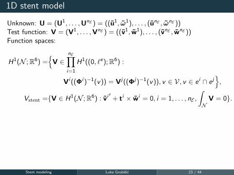
1D stent model: weak formulation revisited

a(U,V) =

nE∑i=1

∫ ì

0QiHi (Qi )T (ωi )′ · w′dx1,

b(V,Ξ) =

nE∑i=1

∫ ì

0ξi · (vi

′+ ti × wi )dx1

+α ·nE∑i=1

∫ ì

0vidx1 + β ·

nE∑i=1

∫ ì

0widx1,

Ξ = (ξ1, . . . , ξnE ,α,β),

f (V) =

nE∑i=1

∫ ì

0fi · vidx1,

M = L2(N ;R3)× R3 × R3 =

nE∏i=1

L2(0, ì ;R3)× R3 × R3

K = Vstent = V ∈ H1(N ;R6) : b(V,Θ) = 0,∀Θ ∈ M.Stent modeling Luka Grubisic 24 / 44

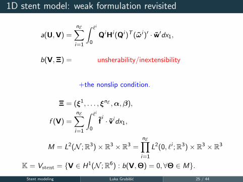
1D stent model: weak formulation revisited

a(U,V) =

nE∑i=1

∫ ì

0QiHi (Qi )T (ωi )′ · w′dx1,

b(V,Ξ) = unsherability/inextensibility

+the nonslip condition.

Ξ = (ξ1, . . . , ξnE ,α,β),

f (V) =

nE∑i=1

∫ ì

0fi · vidx1,

M = L2(N ;R3)× R3 × R3 =

nE∏i=1

L2(0, ì ;R3)× R3 × R3

K = Vstent = V ∈ H1(N ;R6) : b(V,Θ) = 0,∀Θ ∈ M.Stent modeling Luka Grubisic 25 / 44

Evolution problem

pi ′ + fi

= ρiAi∂tt ui ,

qi ′ + ti × pi = 0,

ωi ′ + QiHi (Qi )T qi = 0,

ui ′ + ti × ωi = θi ,

i = 1, . . . , nE + junction conditions

Let (limit of 3D linearized Antman-Cosserat model)

m(U,V) =

nE∑i=1

ρiAi

∫ `i

0ui · vidx1,

Problem (EvoP)

Find U ∈ L2(0,T ;Vstent) such that

d2

dt2m(U,V) + a(U,V) = f (V), V ∈ Vstent.

Eigenvalue problem for 1D stent model Luka Grubisic 26 / 44

Convergence theory by Boffi–Brezzi–Marini

Recall solution operator T : H → Dom(k) and S : H → Dom(B),

k(Tf , uS) + b(Sf , uS) = (f , uS), uS ∈ Dom(k),

b(nS ,Tf ) = 0, nS ∈ Dom(B∗).(4.2)

Disscretization

For a discretization take Xh i Mh as piecewise polynomial spaces on N .Then the discrete solution operators are

k(Thfh, uS) + b(Shf , uS) = (f , uS), uS ∈ Xh,

b(nS ,Tf ) = 0, nS ∈ Mh.(4.3)

The space Kh ⊂ K is the space ov polynomials which satisfy the

constraints.


Convergence theory by Boffi–Brezzi–Gastaldi

Proposition

Let Kh be a nonempty sequence of subspaces for which we haveinperpolation estimates and let k be elliptic on K. Then there isω(h) = o(1) such that

‖Tf − Thf ‖VS≤ ω(h)‖f ‖L2(N ;Z3).

Bounded compact operators Th norm converge to T .

If the resolvent is converging somewhere – say at z = 0 –then it

converges for every z in resolvent set ρ(T ) = C \ Spec(T ).


Convergence rate – coments

Let λ, u and λh and uh be eigenvalues and eigenvectors from Xh

Then

|λ− λh| ≤ C‖T − Th‖Dom(k) = O(ω(h))

‖u − uh‖Dom(k) ≤ C‖T − Th‖Dom(k) = O(ω(h)) .

eigenfuction c.rate optimal, eigenvalue c.rate not.If Sh exists, then

|λ− λh| ≤ C‖T − Th‖Dom(k)‖S − Sh‖ .

λh is a Ritz value of h but not a Ritz value of the solution operator T .


Finite element spaces

00.005

0.010.015

0.02

−2−1

01

2

x 10−3

−1.5

−1

−0.5

0

0.5

1

1.5

x 10−3

• For finite element spaces take

X(n)h = uS ∈ H1(N ;R6) : uS |ei ∈ Pn(ei ;R6), i = 1, . . . , nE,

M(m)h = nS ∈ L2(N ;R6) : nS |ei ∈ Pm(ei ;R3), i = 1, . . . , nE.

• We expect the error behaving as in 1D interpolation.• Piecewise polynomial approximation of the curved middle line?


Convergence rates

• Sobolev spaces on graphs – nice review by O. Post

• Good interpolation operators for lower order spaces – hard because ofthe contact conditions in junctions! Geometry of the graph plays arole.

• For X(n)h ,M

(n−1)h approximation we obtain

(#DOF)−(n+1)

decay rates for the eigenvalue errors.

• for second order problems see Arioli and Benzi 2015.

The interplay of geometry and constraints

Doing interpolation on each edge and then assembling into a graph failsfor first order polynomials since the constraint is to restrictive. Usinghigher order polynomials introduces numerical integration problems inmatrix assembly.


Matrix formulation

For stiffness we have

K =

0 0 0 0 · · · 0 00 A11 0 A12 · · · 0 A1m+1

......

......

. . ....

...0 0 0 0 · · · 0 00 Am+11 0 Am+12 · · · 0 Am+1m+1

, B =

B11 · · · B1n+1

C 11 · · · C 1n+1

... · · ·...

Bm+11 · · · Bm+1n+1

Cm+11 · · · Cm+1n+1

.

and for mass

M =

[M 00 0

]=

D11 0 D12 0 · · · D1m+1 00 0 0 0 · · · 0 0...

......

.... . .

......

Dm+11 0 Dm+12 0 · · · Dm+1m+1 00 0 0 0 · · · 0 0

0

0 0

.

• translations have mass but no stifness• micro-rotations have stifness but no mass• graph connectivity is in B• stifness positive definite on K.


Examples of eigenproblem for 1D stent model

Four stents considered

00.005

0.010.015

0.02

−2−1

01

2

x 10−3

−1.5

−1

−0.5

0

0.5

1

1.5

x 10−3

0

0.01

0.02

−2−1

01

2

x 10−3

−1.5

−1

−0.5

0

0.5

1

1.5

x 10−3

00.005

0.010.015

0.02

−2−1

01

2

x 10−3

−1.5

−1

−0.5

0

0.5

1

1.5

x 10−3

0

0.01

0.02

−1.5−1−0.500.511.5

x 10−3

−1.5

−1

−0.5

0

0.5

1

1.5

x 10−3


Leading eigenvalues

Palmaz Cypher Express Xience

1. 1.033 0.8894 0.06014 0.054882. 1.033 0.8895 0.06014 0.054883. 5.265 1.3683 0.32504 0.287674. 7.499 3.5328 0.33972 0.322015. 7.499 3.5329 0.33973 0.322016. 11.329 3.6604 0.58740 0.58038


Palmaz

−5 0 5 10 15 20

x 10−3

−3

−2

−1

0

1

2

3x 10

−3

−5 0 5 10 15 20

x 10−3

−3

−2

−1

0

1

2

3x 10

−3

−5 0 5 10 15 20

x 10−3

−1.5

−1

−0.5

0

0.5

1

1.5x 10

−3

−5 0 5 10 15 20

x 10−3

−3

−2

−1

0

1

2

3x 10

−3

−5 0 5 10 15 20

x 10−3

−3

−2

−1

0

1

2

3x 10

−3

−2 −1.5 −1 −0.5 0 0.5 1 1.5 2

x 10−3

−2

−1

0

1

2x 10

−3


Cypher

−5 0 5 10 15 20

x 10−3

−3

−2

−1

0

1

2

3x 10

−3

−5 0 5 10 15 20

x 10−3

−3

−2

−1

0

1

2

3x 10

−3

0 0.002 0.004 0.006 0.008 0.01 0.012 0.014 0.016 0.018−2

−1

0

1

2x 10

−3

−5 0 5 10 15 20

x 10−3

−3

−2

−1

0

1

2

3x 10

−3

−5 0 5 10 15 20

x 10−3

−3

−2

−1

0

1

2

3x 10

−3

−4 −3 −2 −1 0 1 2 3 4

x 10−3

−1.5

−1

−0.5

0

0.5

1

1.5x 10

−3


Express

−5 0 5 10 15 20

x 10−3

−3

−2

−1

0

1

2

3x 10

−3

−5 0 5 10 15 20

x 10−3

−3

−2

−1

0

1

2

3x 10

−3

−5 0 5 10 15 20

x 10−3

−2

−1

0

1

2x 10

−3

−5 0 5 10 15 20

x 10−3

−3

−2

−1

0

1

2

3x 10

−3

−5 0 5 10 15 20

x 10−3

−3

−2

−1

0

1

2

3x 10

−3

−5 0 5 10 15 20

x 10−3

−2

−1

0

1

2x 10

−3


Xience

−5 0 5 10 15 20

x 10−3

−3

−2

−1

0

1

2

3x 10

−3

−5 0 5 10 15 20

x 10−3

−3

−2

−1

0

1

2

3x 10

−3

−5 0 5 10 15 20

x 10−3

−2

−1

0

1

2x 10

−3

−5 0 5 10 15 20

x 10−3

−3

−2

−1

0

1

2

3x 10

−3

−5 0 5 10 15 20

x 10−3

−3

−2

−1

0

1

2

3x 10

−3

−5 0 5 10 15 20

x 10−3

−2

−1

0

1

2x 10

−3


Convergence rates — dominated by geometry errors


Exponential integrators

RecallT−1u = ω2Mu .

so let’s use, for u0 ∈ Ker(B),

u = cos((TM)−1/2 t)u0 + (TM)1/2 sin((TM)−1/2 t)u1

for vibration analysis.

For the “heat” equation see Emmrich and Mehrmann

Grimm, Hochbruck, Goeckler (trigonometric integrators) use resolvent

Krylov subspace projection to propagate a very stiff second order system.

Some further developments Luka Grubisic 40 / 44

Exponential integrators

RecallT−1u = ω2Mu .

so let’s use, for u0 ∈ Ker(B),

u = cos((TM)−1/2 t)u0 + (TM)1/2 sin((TM)−1/2 t)u1

for vibration analysis.For the “heat” equation see Emmrich and Mehrmann

Grimm, Hochbruck, Goeckler (trigonometric integrators) use resolvent

Krylov subspace projection to propagate a very stiff second order system.


Trigonometric integrators

Action of T is accessible by solving the saddle-point problem.

For u0, so that ‖u0‖+ ‖Gu0‖ <∞ we have

‖u −Wn(τG 1/2)u0‖ ≤τ C√n‖Gu0‖

where Wn is the rational approximation of the sine or cosine operator fromthe (resolvent) Krylov space

Kn = spanTu0,T2u0, · · · ,T nu0

1D stent simulation


Some conclusions

• Can detect undesirable vibration modes (meshy structures are stiffer,but can unexpectedly buckle).

• For a numerical integration we would like to approximate curved rodby splitting it in a chain of straight rods which approximate themiddle line

• Questions ?I Discrete inf-supI Good linear for Schur complements?


Acknowledgment

Research supported by theCroatian Science Foundationgrant nr. HRZZ 9345


Thank you for your attention!


operator representation of an networks of pdes modeling a

Documents