operating cost for commercial vehicle operators in minnesota · pdf filei thesis: operating...

i

THESIS: Operating Costs for Commercial Vehicle Operators in Minnesota By Maryam Hashami Spring 2004

ii

ACKNOWLEDGEMENTS First and foremost, I would like to express my gratitude to my advisor Dr. David

Levinson, for his expert guidance and suggestion for this thesis. My sincere gratitude

goes to the fellow graduate students who have worked on the Cost/Benefit study for their

support and guidance. I would also like to acknowledge the Minnesota Department of

Transportation and Local Road Research Board for their financial support of the

Cost/Benefit study of Spring Load Restriction policy in Minnesota which this thesis was

part.

iii

ABSTRACT

This study was performed in order to provide information to use in a benefit cost

analysis of the Spring Load Restriction Policy (SLR) in Minnesota. The aim of the study

was to determine the cost of the SLR policy on the freight industry. To do so requires an

estimate of operating cost per km for commercial vehicle operators. A survey of

commercial road users was performed to determine the economic impacts of SLR. The

average operating cost per km for commercial vehicle operators has been calculated from

the responses. A Cobb-Douglas model gives the best fit to estimate the total cost from our

data. From the model one can see roughly constant return to scale occur; if output (total

truckloads) increases by 1%, total cost will increase by 1.05%.

iv

TABLE OF CONTENTS ACKNOWLEDGEMENTS i

ABSTRACT ii

TABLE OF CONTENTS iii

LIST OF FIGURES iv

LIST OF TABLES v

CHAPTER ONE Introduction 1

CHAPTER TWO Survey 4

CHAPTER THREE Operating Cost Models 11

CHAPTER FOUR Summary and Conclusions 24

REFERENCES 26

APPENDIX A 28

v

LIST OF FIGURES Figure 2.1 Histogram of Operating Cost per KM 10

Figure 3.1 Histogram of Average Cost 21

vi

LIST OF TABLES

Table 2.1 Response Rate for Mailed Survey 5

Table 2.2 Summary of Response Rate for Mailed Survey 6

Table 2.3 Route Decision 6

Table 2.4 Financial Penalty 7

Table 2.5 Drivers Compensation 7

Table 2.6 Length of Hauls by Industry 8

Table 2.7 Cost per KM 9

Table 3.1 Correlation Matrix of Variables 15

Table 3.2 Result of Linear Regression and Cobb-Douglas Models 17

Table 3.3 Result of Cobb-Douglas Model by Industry 19

Table 3.4 Economies of scale by variable and industry classification 23

1

Chapter One Introduction

Spring Load Restrictions (SLR) are used in Minnesota as a strategy to reduce the

damage on pavement and to protect investment in road infrastructure by restricting the

weight of heavy trucks during the spring thaw.

During the spring thaw, the soil under the pavement becomes weak; thus, heavy

trucks may cause more pavement damage and reduce pavement life. SLR by reducing

pavement loads should increase road life, but it will also impose costs on the freight

industry. The aim of the study of which this thesis is a part is to determine the cost of

SLR on freight industry and compare it with the cost of repairing roads.

To determine the economic impacts of SLR, a survey of commercial road users is

performed. We find during SLR periods, trucking companies change their operating

behavior mostly by changing routes and reducing load size, which imposes additional

cost on their operation.

Using data collected from our survey, the average operating cost per km for trucks

and value of time are calculated. Truck operating cost per km will be used to determine

the cost of the SLR on the freight industry.

This thesis describes the study and calculates the average and marginal truck

operating cost in Minnesota by using models estimated from data collected from a large

sample of different trucking companies to examine whether trucking firms exhibit

economies of scale in their operation.

2

Transportation cost, including the question of economy of scale, has been of

interest to decision makers in different transportation sectors for many years. Managers

need to have enough information about their costs to make the right decision about the

type of services to provide and the prices to charge (Braeutigam, 1999).

There are many factors that can be used to determine the presence of economies

of scale for firms in the transportation industry. In railroads, economy of scale can be

estimated for traffic density, length of haul, size of firm, number of products. The studies

that were conducted to estimate economies of scale for railroad industry during the 1950s

and 1960s showed there were no economy of size or traffic density. Later studies in

1970s showed increasing returns and economies of traffic density for large railroads

(Keeler, 1983). Results show that to reduce railroad cost, the flow of traffic over existing

lines should increase or the lines with light traffic need to be eliminated.

In the airline industry, cost studies have found the unit cost of service within any

city-pair market decreases quickly, there are roughly constant returns to scale exist for

U.S. trunk carriers, and there are economies of scale for smaller airlines (Keeler, 1983).

Economies of density in the airline industry exist because average costs decline as a plane

filled and because larger planes can move more passengers at a lower average cost.

Most of the studies for motor carriers, for example Winston et al. (1990) and

Allen and Liu (1995), show that they operate subject to constant returns to scale, however

smaller carriers may operate with some increasing retunes to scale (Braeutigam, 1999).

This thesis consists of four chapters. Chapter Two discusses the framework and

process of the survey and provides descriptive results. Chapter Three estimates a cost

3

model from the survey data. Chapter Four summarizes the findings and presents

conclusions.

4

Chapter Two Survey This chapter will discuss the survey to determine the effect of SLR on the freight

industry in Minnesota. First it will discuss the objective of the survey, the population

sample and the survey methodology, then it will discuss the statistical results obtained

from the survey.

The objective of the survey was to appraise the effect of SLR on freight

transportation among different sectors of the freight industry and collect some general

information about their operation. The survey collected data which was believed to affect

value of time and operating cost per mile, such as size of company, type of trucks and

company strategy.

Data were collected for different trucking companies in Minnesota. The target

was the decision maker in each company, who was thought to be able to give accurate

information of how their trucks operate. Contact information was obtained from different

sources: Minnesota Department of Transportation (Mn/DOT) Freight Facilities Database,

Minnesota Trucking Association (MTA) board of directors, Mn/DOT overweight permit

list, Mn/DOT filed insurance list, and a list of trucking company in Minnesota from city

and county engineers. Table 2.1 displays our response rate results.

5

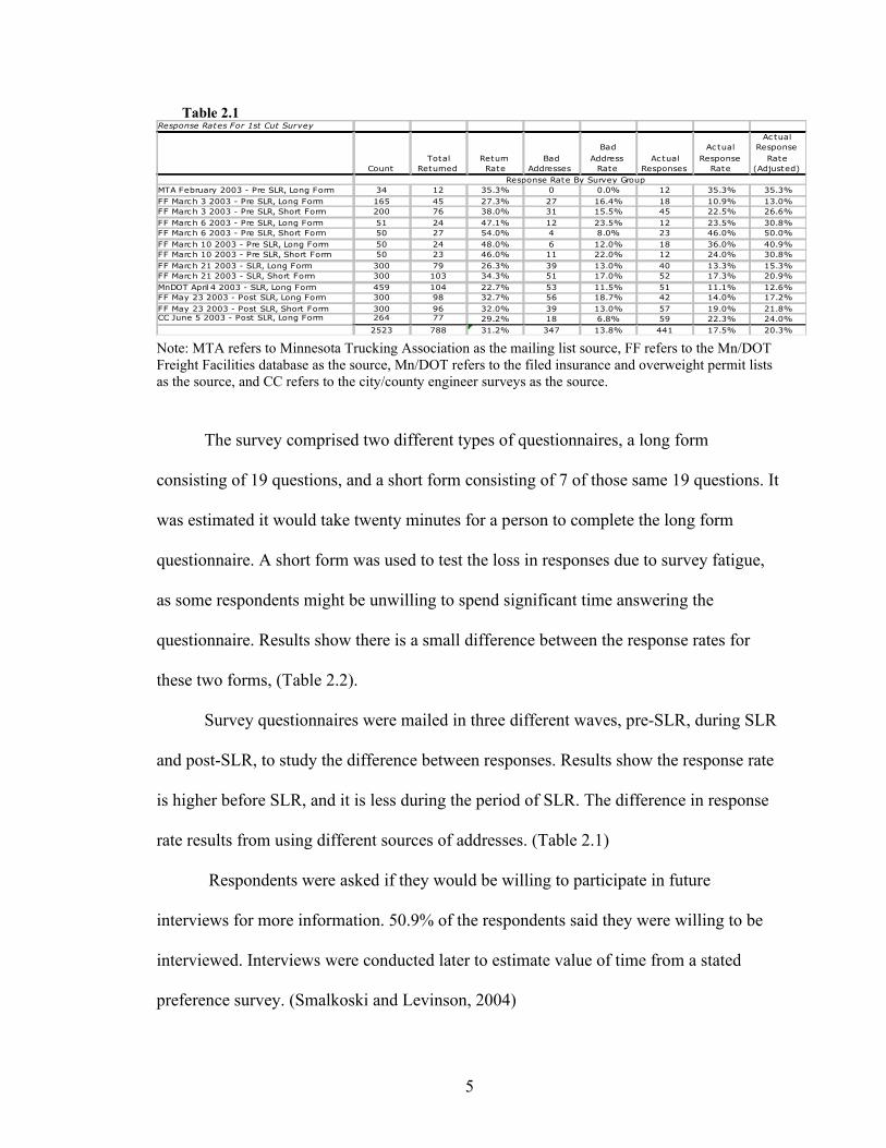
Table 2.1 Response Rates For 1st Cut Survey

Count

Total

Returned

Return

Rate

Bad

Addresses

Bad

Address

Rate

Ac tual

Responses

Ac tual

Response

Rate

Ac tual

Response

Rate

(Adjusted)

MTA February 2003 - Pre SLR, Long Form 34 12 35.3% 0 0.0% 12 35.3% 35.3%

FF March 3 2003 - Pre SLR, Long Form 165 45 27.3% 27 16.4% 18 10.9% 13.0%

FF March 3 2003 - Pre SLR, Short Form 200 76 38.0% 31 15.5% 45 22.5% 26.6%





FF March 21 2003 - SLR, Long Form 300 79 26.3% 39 13.0% 40 13.3% 15.3%

FF March 21 2003 - SLR, Short Form 300 103 34.3% 51 17.0% 52 17.3% 20.9%

MnDOT April 4 2003 - SLR, Long Form 459 104 22.7% 53 11.5% 51 11.1% 12.6%

FF May 23 2003 - Post SLR, Long Form 300 98 32.7% 56 18.7% 42 14.0% 17.2%

FF May 23 2003 - Post SLR, Short Form 300 96 32.0% 39 13.0% 57 19.0% 21.8%CC June 5 2003 - Post SLR, Long Form 264 77 29.2% 18 6.8% 59 22.3% 24.0%

2523 788 31.2% 347 13.8% 441 17.5% 20.3%

Response Rate By Survey Group

Note: MTA refers to Minnesota Trucking Association as the mailing list source, FF refers to the Mn/DOT Freight Facilities database as the source, Mn/DOT refers to the filed insurance and overweight permit lists as the source, and CC refers to the city/county engineer surveys as the source.

The survey comprised two different types of questionnaires, a long form

consisting of 19 questions, and a short form consisting of 7 of those same 19 questions. It

was estimated it would take twenty minutes for a person to complete the long form

questionnaire. A short form was used to test the loss in responses due to survey fatigue,

as some respondents might be unwilling to spend significant time answering the

questionnaire. Results show there is a small difference between the response rates for

these two forms, (Table 2.2).

Survey questionnaires were mailed in three different waves, pre-SLR, during SLR

and post-SLR, to study the difference between responses. Results show the response rate

is higher before SLR, and it is less during the period of SLR. The difference in response

rate results from using different sources of addresses. (Table 2.1)

Respondents were asked if they would be willing to participate in future

interviews for more information. 50.9% of the respondents said they were willing to be

interviewed. Interviews were conducted later to estimate value of time from a stated

preference survey. (Smalkoski and Levinson, 2004)

6

Table 2.2 Summary Response Rates For 1st Cut Survey

Count

Total

Returned

Return

Rate

Bad

Addresses

Bad

Address

Rate

Ac tual

Responses

Ac tual

Response

Rate

Ac tual

Response

Rate

(Adjusted)

Long Form 1623 463 28.5% 211 13.0% 252 15.5% 17.8%

Short Form 900 325 36.1% 136 15.1% 189 21.0% 24.7%

Pre SLR (MTA, FF) 600 231 38.5% 91 15.2% 140 23.3% 27.5%

SLR (FF& MnDOT) 1059 286 27.2% 143 13.5% 143 13.5% 15.6%

Post SLR (FF, CC) 864 271 31.4% 113 13.1% 158 18.3% 21.0%

Response Rate By Wave

Response Rate By Form Type

Important information was obtained from the survey, including: type of trucks

and number of axles, overall distance traveled by a firm’s trucks, number of employees,

type of products that a firm hauls, if the company is assessed financial penalties for late

or missed delivery, who chooses the route, total truckloads per year, operating cost per

unit distance, if they impose a fuel surcharge, and how do they pay their drivers.

Table 2.3 summarizes the results of who chooses the routes traveled by trucks. It

shows in most cases the driver is the one who decides about the routes. Some

respondents chose multiple decision makers.

Table 2.3 Route Decision

Management 26.0%

Dispatcher 10.0%

Driver 43.0%

Management & Dispatcher 1.0%

Management & Driver 7.5%

Driver & Dispatcher 9.0%

Management & Driver & Dispatcher 3.5%

Table 2.4 shows the percentage of companies who were assessed financial

penalties for late/missed deliveries. It seems average cost per km for companies that

assessed penalties are higher than others.

7

Table 2.4 Financial Penalties

Assessed Financial Penalties For Late/Missed Deliveries 24.8%

Cost/Km if Assessed Penalties $0.81

Cost/Km if not Assessed Penalties $0.63

Table 2.5 displays the way that driver compensation was determined. Some

respondents chose multiple compensation methods, but most drivers were paid on an

hourly basis.

Table 2.5 Driver Compensation

Load 15.0%

Time 55.0%

Distance 14.0%

Distance & Load 4.0%

Distance & Time 6.0%

Load & Time 2.0%

Load & Time & Distance 1.1%

% of Profits 2.9% Results show only 14.8% of trucking companies linked their driver compensation

to on-time deliveries. Almost half of the sample imposed a fuel surcharge.

Table 2.6 summarizes the results of average trip length per truck load by industry.

Truck loads are assumed to be round trips. Results show food products have the most km

per truckload compared to other industries.

8

Table 2.6 Km/Truckload

Km/Truckload Response Count

Average 503 198

Food Products 1446 15

Industrial Supplies 1058 16

General Products 989 23

Dairy 635 3

Construction 392 10

Timber 379 10

Paper 354 4

Agricultural 312 61

Beverages 259 3

Petroleum 235 12

Rubbish 161 3

Ag Chem 151 14

Aggregate 66 23

By Industry

The average cost per km from data collected was $0.69. This was for a sample

of 186 different trucking companies. The answers ranged between $0.087 and $2.98

which shows the diversity of cost per km by industry and size of company (see figure 1).

If we assume labor cost per km for commercial trucks to be $0.22, values below $0.31

can not be correct and may exclude labor cost. We suspect that the data around $0.69

more accurately represents the total cost of operating a truck per km, such that the

respondents correctly interpreted the question as total cost including labor. A follow up

study was conducted to get a better result for cost per km. All respondents who had

operating cost per km less than $0.31 were contacted by the phone to verify their

answers. There were total of 26 responses less than $0.31.

We verified seven of them. Five of them changed after the follow up study. None of the

responses has been removed from our data, as we were not certain they were incorrect.

9

Owner/operators have higher operating cost compared to non owner/operators,

perhaps a result of having fewer trucks to distribute their fixed operating costs over. If

economies of scale exist, it makes sense that smaller firms have higher operating cost.

See Table 2.7. Figure 2.1 displays a histogram of cost/km.

Table 2.7

Cost/Km

Response

Count Average Mode Median

Standard

Deviation

Overall 186 $0.69 $0.62 $0.60 $0.44

Rubbish 2 $1.54 $1.54 $1.30

Dairy 3 $1.03 $0.84 $0.47

Food Products 18 $0.90 $0.60 $0.64 $0.66

Paper 4 $0.85 $0.86 $0.29

Petroleum 11 $0.81 $1.86 $0.78 $0.62

Timber 5 $0.76 $0.56 $0.40

Aggregate 22 $0.70 $0.30 $0.61 $0.37

Industrial Supplies 12 $0.68 $0.56 $0.59 $0.43

Construction 13 $0.67 $0.40 $0.59 $0.35

Ag Chem 15 $0.62 $0.80 $0.48 $0.67

Agricultural 55 $0.61 $0.50 $0.55 $0.32

General Products 24 $0.60 $0.78 $0.65 $0.29

Beverages 2 $0.50 $0.50 $0.54

Owner/Operator 21 $0.84 $0.93 $0.50 $0.69

Non Owner/Operator 165 $0.67 $0.80 $0.61 $0.39

By Industry

Owner/Operator

10

0

10

20

30

40

50

60

0 0.25 0.5 0.75 1 1.25 1.5 1.75 2 2.25 2.5 2.75 3 More

Cost per km ($)

Frequency

Figure 2.1 Histogram of Operating Cost Per Km

11

Chapter Three Operating Cost Models

There are many approaches to estimate the cost per km for trucks. Each of them

employs a different methodology and models to calculate the variable costs of operating

trucks. Fuel, repair and maintenance, tire, depreciation, and labor cost are the most

important costs that are considered to estimate operating cost per km.

Daniels (1974) divided vehicle operating cost into two different categories,

running costs and standing cost. Running cost includes fuel consumption, engine oil

consumption, tire costs, and maintenance cost. Standing cost includes license, insurance,

interest charges. He mentioned speed as the most important factor in fuel consumption

and found maintenance costs rise with increasing speed. If fuel consumption and

maintenance cost change, operating cost will change as well. Vehicle size is another

factor that affects fuel consumption and it will change operating cost. By using average

axle number for each firm we can include vehicle size in our model.

Watanatada (1987) divided the variables that affect the truck operating cost to the

following categories:

1) Truck characteristics e.g., weight, engine power, maintenance

2) Local factors e.g., speed limit, fuel price, labor cost, drivers attitude

3) Road characteristics e.g., pavement roughness, road width

Operating Cost is considered a function of road characteristics and so is policy sensitive.

Barnes (2003) estimated operating cost for commercial trucks based on fuel,

repair, maintenance, tires and depreciation costs. He also considered adjustment factors

for cost, based on pavement roughness, driving conditions and fuel price changes. He

12

estimated average of truck operating cost per km is $0.27 cents, not including labor cost.

If we assume labor cost is around $0.22 per km, total operating cost using Barnes model

will be around $0.49 per km. We can use this number as a check for operating cost per

km data that we obtained from the survey.

Truck Operating Cost Model

Theory

Firms seek to minimize their cost including truck operating cost. Truck operating

cost for each firm can be divided into fixed and variable costs. Fixed costs are not

sensitive to the volume of output, but variable costs change with the level of output.

Waters (1997) has explained different costing methods that are useful to estimate

the relationship between outputs and costs. One of the methods that has been used in

transportation studies is the statistical costing method. In this method the relationship

between outputs and costs will be estimated using statistical techniques across

observations. Multiple regression analysis shows how cost changes by changing any of

the variables. In our study the statistical method will be used to estimate the effect of

different variables on operating cost.

The factors which are posited to be important in estimating total operating cost for

different firms follow:

13

Size of firm:

Economies of scale in larger firms would reduce operating cost. This means larger

companies should have a lower cost per unit distance. In this case two factors give us size

of firm: km per truckload and number of truckloads. They are important factors and they

are expected to be significant in our model. Km/Truckload ( TK / ) is calculated by

dividing the total kilometers traveled by firm’s truck in a year by total annual truckloads.

It measures average length of haul for each firm. We expect it will be statistically

significant in our model as total cost should increase by increasing km/load. The Number

of Truckloads (T ) was asked directly from each firm and is another indicator of the size

of the firm. We expect it will be statistically significant and the total cost increases with

number of truckloads.

Firm Strategy:

Each firm develops its own strategy based on management policy, which may

lead to differences in operating costs for firms. In our study we asked if the firm was

assessed financial penalties by clients for late or missed delivery. We also asked how

they determine driver compensation and if compensation is linked to on-time delivery,

and if the firm has a fuel surcharge. All these policies could be used as variables in our

model. Financial Penalty (P ) indicates the company was assessed a financial penalty by

clients for late or missed deliveries. By paying a financial penalty to the client, operating

costs should increase, so we expect it will be positive and significant.

14

Type of Firm:

Different industries have different lengths of haul for their products. Industries

like aggregate and rubbish have shorter trips than others. Owner/operator (O ) indicates

the company owns and operates its own trucks. From survey results we saw the

difference in operating cost for owner/operators versus non owner/operators.

Owner/operators have larger cost per km. The reason for this may be the absence of

economies of scale and that they have fewer trucks over which to distribute their firm’s

fixed costs. The models are estimated separately for each type of firm.

Economy of Scope:

A firm is said to operate with economy of scope if for outputs1y and

2y

)0,(),0(),( 1221 yCyCyyC +< (3.1)

That means the cost of producing two outputs with one firm is less than the cost of

producing each output with two different firms. In our case economy of scope has been

tested by considering the number of goods that a firm hauls as an output. An indicator for

multi-product firms (H ) indicates if a firm hauls more than one good. UsingH as a

dummy variable in the model allows us to test if economies of scope exist in the trucking

industry.

Total Cost Model

To measure the effects of the hypothesized independent variables, we estimate

statistical models with total operating costs as the dependent variable. Total Operating

Cost (C ) is calculated by using this formula:

15

)/(* KCKC = (3.2)

Where:C is cost, K is overall kilometers, and KC / is cost per kilometer.

Both overall kilometers and operating cost per km have been asked directly of each

firm.

Linear Regression model

First a linear model is tested with OLS regression. Using total cost as a dependent

variable and entering independent variables we have following model.

HOPTTKC 543210 )/( !!!!!! +++++= (3.3) Where: C is Total Annual Cost

K is kilometers

T is number of truckloads

P is 1 if firm is assessed a financial penalty for late delivery, 0 otherwise

O is 1 if the firm is owner/operator, 0 otherwise

H is 1 if the firm hauls more than one product, 0 otherwise

From the correlation matrix (Table 3.1), one can see number of truckloads (T ) is highly

correlated with number of drivers (D ) and overall kilometers (K ), because all of them

represent size of firm, just one of them is used in the model.

T D K P O )/( TK H

_______________________________________________________________________________________

T 1.0000 D 0.7441 1.0000 K 0.3867 0.7418 1.0000 P 0.3108 0.3088 0.2520 1.0000 O -0.1207 -0.1289 -0.0748 -0.1710 1.0000 )/( TK -0.0417 -0.0185 0.0076 -0.0245 -0.0116 1.0000 H -0.0134 0.0254 0.0324 -0.0634 -0.1447 -0.1877 1.0000 ___________________________________________________________________ Table 3.1 Correlation Matrix

16

Cobb-Douglas Model

Cobb-Douglas models are often used to estimate cost functions and may provide a better

fit than the linear model.

The form of the Cobb-Douglas model we use: 543210 )()()()/(

!!!!!! HOPeeeTTKeC = (3.4)

The coefficient ! on the independent variable is the elasticity of cost with respect to that

independent variable such as output. It shows the percentage change in total cost resulting

from a 1 percent increase in the level of output.

Using a Cobb-Douglas model we have following: )()()()()/()( 543210

HOPeLneLneLnTLnTKLnCLn !!!!!! +++++= (3.5)

The results from fitted models are show in Table 3.2

17

Table 3.2 Estimated Models of Total Operating Cost From Table 3.2, we see that the linear model is not a good fit for our data, just two of the

independent variables are significant and the R-squared is 0.180. In the Cobb-Douglas

model three independent variables are statistically significant with p-value less than 0.05,

R-squared is about 0.95.

Results show the elasticity of total cost with respect to the km/load and truckload

is close to 1, (the coefficient on TKLn /( ) and )(TLn ), which means that as the km/load

Model Linear Model Cobb-Douglas Model

Variable

(K/T) ß 45.27 1.015

Std-Error 117.130 0.033

t-stat 0.390 30.620

p-value 0.700 0.000

T ß 117.34 1.043

Std-Error 28.8 0.029

t-stat 4.07 35.87

p-value 0.000 0.000

P ß 3973163 0.297

Std-Error 1791364 0.118

t-stat 2.22 2.52

p-value 0.028 0.013

O ß -43952.11 0.312

Std-Error 2597629 0.172

t-stat -0.02 1.81

p-value 0.987 0.072

H ß 1095115 -0.012

Std-Error 2100002 0.13

t-stat 0.52 -0.09

p-value 0.603 0.927

R-Squared 0.180 0.945

n 145 145

18

rate or truckload rate increase by 1 percent, the total cost will increase roughly by 1

percent as well, which is expected. However coefficients are slightly greater than 1,

indicating overall diseconomies. The coefficients on )( PeLn and )( O

eLn show the

elasticity of total cost with respect to two dummy variables: O andP . Total cost increases

with both variables. Because the coefficients are smaller than 1, it means if the variables

increase by 1 percent, cost increases by 0.3 percent. The coefficient on )( HeLn is

statistically insignificant and indicates no economies of scope.

To determine if the Cobb-Douglas is a good fit for our data, we can look at the

summary graph of the final model. Figure 3.1 shows the actual values versus predicted

values. Results show the predicted total cost by using the Cobb-Douglas model is close to

the actual values.

$0

$20,000,000

$40,000,000

$60,000,000

$80,000,000

$100,000,000

$120,000,000

$0 $20,000

,000

$40,000

,000

$60,000

,000

$80,000

,000

$100,00

0,000

$120,00

0,000

$140,00

0,000

$160,00

0,000

$180,00

0,000

Predicted cost ($)

Total Cost ($)

Figure 3.1 Actual total costs versus predicted total costs from model

R2=0.98

19

To determine if economies of scale exist in the trucking industry we can look at

each industry type individually. Models 3-6 show the results of the Cobb-Douglas model

for four industry types that had a large number of observations.

Table 3.3 Cobb-Douglas estimate of total cost for different industry

Industry Agriculture General Product Aggregate Food Product

Variable

(K/T) ß 1.047 1.023 0.718 0.509

Std-Error 0.050 0.145 0.120 0.227

t-stat 20.910 7.070 5.960 2.240

p-value 0.000 0.000 0.000 0.055

T ß 1.102 1.125 0.809 0.905

Std-Error 0.043 0.083 0.119 0.182

t-stat 25.630 13.500 6.800 4.980

p-value 0.000 0.000 0.000 0.001

P ß 0.214 0.355 0.712 0.128

Std-Error 0.161 0.440 0.354 0.446

t-stat 1.330 0.810 2.100 0.290

p-value 0.191 0.433 0.075 0.782

O ß 0.659 0.179 -0.317 0.364

Std-Error 0.227 0.353 0.626 0.657

t-stat 2.910 0.510 -0.510 0.550

p-value 0.006 0.622 0.625 0.595

H ß -0.339 -0.498 0.250 0.807

Std-Error 0.191 0.302 0.428 0.470

t-stat -1.780 -1.650 0.580 1.720

p-value 0.084 0.124 0.574 0.124

Constant ß -1.404 -1.390 2.016 3.026

Std-Error 0.441 1.171 1.299 2.481

t-stat -3.180 -1.650 1.550 1.220

p-value 0.003 0.124 0.155 0.257

R-Squared 0.970 0.967 0.917 0.944

n 45 19 15 14

20

The coefficients of km/truckload and number of truckload for Agriculture and

General Products are greater than 1, this shows there are diseconomies of scale in

Agriculture and General Products. Diseconomies of scale in Agriculture and General

Products may be the result of smaller firms, more owner/operators or having shorter

hauls. However there are economies of scale in Food Products and Aggregate which may

be a result of larger firm size and longer hauls. (See Table 2.6)

Average Cost Function

The average cost function is found by computing total costs per unit of output.

Assuming total truckloads is the output of each firm, the average cost function for each

firm can be calculated as following:

Average cost = (total cost) / (total truckload)

Average cost: TeeeTTKeTCHOP/))/((/ 543210 !!!!!!

= (3.6)

Average cost: = HOPeeeTKe 5431210 1 !!!!!!! "" (3.7)

HOPeeeTKe

012.0312.0297.0972.0015.1037.1 !!!= (3.8)

Using the mean of each variable in equation (3.8), gives an average cost of $232 per

truckload.

To compare this value with the average cost from survey data, we can use the

mean of cost per km and the mean of overall kilometers to calculate the average total

cost. Average cost can be calculated by dividing average total cost by average truckload

(output). This gives an average cost of $249 per truckload.

21

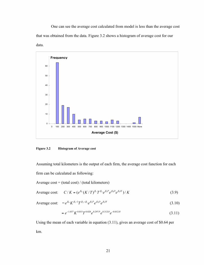
One can see the average cost calculated from model is less than the average cost

that was obtained from the data. Figure 3.2 shows a histogram of average cost for our

data.

Figure 3.2 Histogram of Average cost

Assuming total kilometers is the output of each firm, the average cost function for each


Average cost = (total cost) / (total kilometers)

Average cost: KeeeTTKeKCHOP/))/((/ 543210 !!!!!!

= (3.9)

Average cost: = HOPeeeTKe 5431210 1 !!!!!!! "" (3.10)

HOPeeeTKe

012.0312.0297.0028.0015.0037.1 !!= (3.11)

Using the mean of each variable in equation (3.11), gives an average cost of $0.64 per

km.

0

10

20

30

40

50

60

0 100 200 300 400 500 600 700 800 900 1000 1100 1200 1300 1400 1500 More Average Cost ($)

Frequency

22

Marginal cost function

The marginal cost function is found by computing the change in total costs for a

change in output. If output is total truckloads then: Marginal cost = (change in total cost) / (change in truckloads)

The marginal cost function is TC !! / = HOPeeeTKe 5431210 1

12 )(!!!!!!!!! """ (3.12)

Using coefficients from Table 3.2, the marginal cost function will be

HOPeeeTKeMC

012.0312.0297.0972.0015.1037.1)015.1043.1( !!!!= (3.13)

Using the mean of each variable in equation (3.13), gives an overall marginal cost per

truckload of $6.51. The average cost per truckload is much higher than the marginal cost,

indicating economies of scale in truckloads.

Assuming total kilometers is the output of each firm, the marginal cost function for each


The marginal cost = (change in total cost) / (change in kilometers)

Marginal cost function is KC !! / = HOPeeeTKe 5431210 1

1

!!!!!!!! "" (3.14)

Using coefficients from Table 3.2, the marginal cost function will be

HOPeeeTKeMC

012.0312.0297.0028.0015.0037.1015.1

!!= (3.15)

Using the mean of each variables in equations (3.15), can give us an overall marginal cost

per km of $0.65.

23

The marginal cost is slightly higher than the average cost, indicating slight

diseconomies of scale per km. Table 3.4 summarizes economies of scale by variable and

industry classification.

Table 3.4 Economies of scale by variable and industry classification

Industry Agriculture General Product Aggregate Food Product

Variable

AC per truckloads 188.00 597.00 20.00 588.00

MC per truckloads 9.94 60.93 1.80 233.18

Economies of scale 18.90 9.79 11.11 2.52

AC per km 0.67 0.76 0.54 0.66

MC per km 0.70 0.78 0.37 0.33

Economies of scale 0.95 0.97 1.46 2.00

24

Chapter Four

Summary and Conclusions

The average cost per km for commercial trucks in Minnesota is $ 0.69. This

number is the result of using data collected from 186 different firms in Minnesota.

Owner/operators have a higher cost as a result of having less output to distribute their

fixed cost over.

A Cobb-Douglas model gives the best fit to estimate the total cost from our data.

Total truckloads represent the size of firm in the total cost model. From the model one

can see roughly constant return to scale. If output (total truckloads) increases by 1%, total

cost will increase by 1.04%. Results from the model for each industry type show there are

economies of scale in food product and aggregate industry. It may be result of having

longer length of hauls or larger firms.

Average cost for trucks obtained from the model is $0.64 per km. That is very

close to the average cost from our data. Average cost per truckload is about $250 per

truckload. Marginal cost per truckload is $6.51 and Marginal cost per km is $0.65.

Therefore there are economies of scale in additional truckloads but diseconomies in

additional km.

A caveat on the analysis is that some of the respondents may have misunderstood

the survey questionnaire. We suspect the numbers of respondents (26 of 186) who

reported operating cost less than 0.3 per km may not include labor cost in their answers.

This may cause our estimate to be somewhat lower than the actual number.

25

The total operating cost model estimation also doesn’t show the impact of road

quality on operating cost. It may be an important factor in operating cost as low quality

roads can reduce the life of tires, increase fuel consumption and also increase the

maintenance cost. It may also reduce speed which increases labor cost.

26

References

Barnes, G., Langworthy, P., (2003), The Per-Mile Costs of Operating Automobiles and Trucks. Forthcoming report, Minnesota Department of Transportation. Braeutigam, R. R., (1999), Learning about Transport Costs, In Gomez-Ibanez, J. A., Tye, W. B., Winston, C., (Editors), Essay in Transportation Economics and Policy, Brooking Institution Press, Washington, D.C. Chesher, A., Harrison, (1987), Vehicle Operating Cost, The Johns Hopkins University Press Baltimore and London (published for the world bank) Daniels, C., (1974), Vehicle operating costs in transport studies: With special reference to the work of the EIU in Africa. Economist Intelligence Unit, London. Edwards, S. L., Bayliss, B. T., (1970), Operating Costs in Road Freight Transport. Greene, W. H., (2000), Econometric Analysis, New York University. Lansing, J. B., Morgan, J. N., (May 1971), Economic Survey Methods, University of Michigan. Levinson, D., Smalkoski, B,. (2003), Value of time for Commercial Vehicle Operators in Minnesota, Transportation Research Board International Symposium on Road Pricing, Key Biscayne, Florida, November. Nicholson, W., (1998), Microeconomic Theory Basic Principles and Extensions, Amherst College. Kawamura, K., (1999), Commercial Vehicle Value of Time and Perceived Benefit of Congestion Pricing. Institute of Transportation Studies, University of California at Berkeley.

27

Keeler, T. E., (1983), Railroad, Freight, and Public Policy, Brookings Institution, Ch.3 (Competition, Natural Monopoly, and Scale Economies), pp. 43-61 Thoresen, T., Roper, R., (1996), Review & enhancement of Vehicle Operating Cost models: Assessment of non urban evaluation models, ARRB Transport Research Ltd. Watanatada , T., Dhareshwar, A. M.,(1987), Vehicles Speeds and Operating Costs, Washington, D.C., The World Bank. Waters, W. G., (Spring, 1976), Statistical Costing in Transportation, Transportation Journal, pp. 49-62.

28

Appendix A

Mailed Survey

Please complete: Contact Name ____________________________ Name of Firm ____________________________ Street Address ____________________________ City, State, Zip ____________________________ Phone Number (____) ______________________ E-mail Address ____________________________ Date Completed ____________

1. How many trucks does your firm operate? Truck Type Total Number of Axles

2 3 4 5 6 7 8 Pickups/Light Duty Trucks ____ ____ Unibody Dock Truck ____ ____ Platform & Flatbed ____ ____ ____ ____ ____ ____ ____ Dry Bulk (Hopper, dump, etc.) ____ ____ ____ ____ ____ ____ ____ Liquid/Gas Tank ____ ____ ____ ____ ____ ____ ____ Refrigerated Van ____ ____ ____ ____ ____ ____ ____ Livestock Van ____ ____ ____ ____ ____ ____ ____ Dry Van ____ ____ ____ ____ ____ ____ ____ Grain Body ____ ____ ____ ____ ____ ____ ____ Dump Truck ____ ____ ____ ____ ____ ____ ____ Concrete Mixer ____ ____ ____ ____ ____ ____ ____ Pole & Logging ____ ____ ____ ____ ____ ____ ____ Other, please specify__________ ____ ____ ____ ____ ____ ____ ____

2. How many miles did your firm’s trucks travel over the course of 2002?

Total? __________, in Minnesota? __________

3. Please list general types of major commodities/products that your firm hauls.

__________, __________, ___________, __________, __________

4. How many direct employees does your firm have? __________

29

5. How many of the direct employees are drivers? __________

6. How many drivers are contracted / leased by your firm? __________

7. Who chooses the routes traveled by the trucks? Please indicate choice by circling.

Management Dispatcher Driver Other, please specify

8. Is your company assessed financial penalties by clients for missed/late delivery or pickup time? Please check one. □ Yes □ No 9. How is driver’s compensation determined? Please indicate choice by circling.

Load Time Miles Other, please specify

10. Is driver compensation linked to on-time deliveries? □ Yes □ No

11. Do you change the rate you charge clients to account for the fluctuations in gas/diesel price? □ Yes □ No

12. What is your approximate cost of operating each truck per mile? __________

13. How many truck loads did your firm carry in the past year? ___________

14. Do spring load restrictions affect your firm, and if yes please answer in which ways you change your operations to conform to the seasonal restrictions?

□ Shift the seasonal timing of shipments □ Reduce load size / weight per vehicle □ Increase the number of vehicles used □ Change the kind of vehicles used □ Change routes Other, please specify _______________

30

15. Roughly, what is the percentage of miles that your firm’s trucks spend on roads subject to spring load restrictions? __________

16. How many times were your firm’s trucks cited last year for weight violations

during the period of spring load restrictions? __________

17. Which road(s) are problematic for your firm during spring load restrictions (specific roads, and/or classifications, 5-ton, 7-ton, 9-ton)? Please list.

___________, __________, ___________, ___________, __________

18. Can we contact you at a later date to set-up an interview for additional questions? The interview should take no more than 30 minutes. □ Yes □ No

19. Please indicate by highlighting on the map provided on the back of this page,

which counties your firm’s trucks typically drive in?

operating cost for commercial vehicle operators in minnesota · pdf filei thesis: operating...

Documents