Author: Brenda Gunderson, Ph.D., 2015

License: Unless otherwise noted, this material is made available under the terms of the Creative Commons Attribution-NonCommercial-Share Alike 3.0 Unported License: http://creativecommons.org/licenses/by-nc-sa/3.0/

The University of Michigan Open.Michigan initiative has reviewed this material in accordance with U.S. Copyright Law and have tried to maximize your ability to use, share, and adapt it. The attribution key provides information about how you may share and adapt this material.

Copyright holders of content included in this material should contact open.michigan@umich.edu with any questions, corrections, or clarification regarding the use of content.

For more information about how to attribute these materials visit: http://open.umich.edu/education/about/terms-of-use. Some materials are used with permission from the copyright holders. You may need to obtain new permission to use those materials for other uses. This includes all content from:

Attribution Key

For more information see: http:://open.umich.edu/wiki/AttributionPolicy

Content the copyright holder, author, or law permits you to use, share and adapt:

Creative Commons Attribution-NonCommercial-Share Alike License Public Domain – Self Dedicated: Works that a copyright holder has dedicated to the public domain.

Make Your Own Assessment

Content Open.Michigan believes can be used, shared, and adapted because it is ineligible for copyright.

Public Domain – Ineligible. Works that are ineligible for copyright protection in the U.S. (17 USC §102(b)) *laws in your jurisdiction may differ.

Content Open.Michigan has used under a Fair Use determinationFair Use: Use of works that is determined to be Fair consistent with the U.S. Copyright Act

(17 USC § 107) *laws in your jurisdiction may differ.

Our determination DOES NOT mean that all uses of this third-party content are Fair Uses and we DO NOT guarantee that your use of the content is Fair. To use this content you should conduct your own independent analysis to determine whether or not your use will be Fair.

Statistics 250

Interactive Lecture Notes

Fall 2015

Dr. Brenda GundersonDepartment of StatisticsUniversity of Michigan

Table of Contents

Topic Page

Intro 1

1: Summarizing Data 3

2: Sampling, Surveys, and Gathering Useful Data 25

3: Probability 35

4: Random Variables 45

5: Learning about a Population ProportionPart 1: Distribution for a Sample ProportionPart 2: Estimating Proportions with ConfidencePart 3: Testing about a Population Proportion

657181

6: Learning about the Difference in Population ProportionsPart 1: Distribution for a Difference in Sample ProportionsPart 2: Confidence Interval for a Difference in Population ProportionsPart 3: Testing about a Difference in Population Proportions

939799

7: Learning about a Population MeanPart 1: Distribution for a Sample MeanPart 2: Confidence Interval for a Population MeanPart 3: Testing about a Population Mean

103111117

8: Learning about a Population Mean DifferencePart 1: Distribution for a Sample Mean DifferencePart 2: Confidence Interval for a Population Mean DifferencePart 3: Testing about a Population Mean Difference

127131135

9: Learning about the Difference in Population MeansPart 1: Distribution for a Difference in Sample MeansPart 2: Confidence Interval for a Difference in Population MeansPart 3: Testing about a Difference in Population Means

139143151

10: ANOVA: Analysis of Variance 159

11: Relationships between Quantitative Variables: Regression 171

12: Relationships between Categorical Variables: Chi-Square 193

Stat 250 Gunderson Lecture NotesIntroduction

Statistics...the most important science in the whole world: for upon it depends the practical application of every other science and of every art: the one science essential to all political and social administration, all education, all organization based on experience, for it only gives results of our experience." Florence Nightingale, Statistician

Definitions:

Statistics are numbers measured for some purpose.

Statistics is a collection of procedures and principles for gathering data and analyzing information in order to help people make decisions when faced with uncertainty.

Course Goal: Learn various tools for using data to gain understanding and make sound decisions about the world around us.

1

2

Stat 250 Gunderson Lecture Notes1: Summarizing Data

“ You must never tell a thing. You must illustrate it. We learn through the eye and not the noggin."

--Will Rogers (1879 - 1935)

“Simple summaries of data can tell an interesting story and are easier to digest than long lists.” So we will begin by looking at some data.

Raw DataRaw data correspond to numbers and category labels that have been collected or measured but have not yet been processed in any way. On the next page is a set of RAW DATA - information about a group of items in this case, individuals. The data set title is DEPRIVED and has information about a sample size of n = 86 college students. For each student we are provided with their answer to the question: “Do you feel that you are sleep deprived?” (yes or no), and their self reported typical amount of sleep per night (in hours). The information we have is organized into variables. In this case these 86 college students are a subset from a larger population of all college students, so we have sample data.

Definition: A variable is a characteristic that differs from one individual to the next.

Sample data are collected from a subset of a larger population.

Population data are collected when all individuals in a population are measured.

A statistic is a summary measure of sample data.

A parameter is a summary measure of population data.

Types of VariablesWe have 2 variables in our data set. Next we want to distinguish between the different types of ariables - different types of variables provide different kinds of information and the type will guide what kinds of summaries (graphs/numerical) are appropriate.

3

Think about it: Could you compute the “AVERAGE AMOUNT OF SLEEP”

for these 86 students? Could you compute the “AVERAGE SLEEP DEPRIVED STATUS”

for these 86 students?

SLEEP DEPRIVED STATUS is said to be a variable,

AMOUNT OF SLEEP is a variable.

Definitions: A categorical variable places an individual or item into one of several groups or categories. When the categories have an ordering or ranking, it is called an ordinal variable.

A quantitative variable takes numerical values for which arithmetic operations such as adding and averaging make sense. Other names for quantitative variable are: measurement variable and numerical variable.

Try It! – For each variable listed below, give its type as categorical or quantitative.

Age (years)

Typical Classroom Seat Location (Front, Middle, Back)

Number of songs on an iPod

Time spent studying material for this class in the last 24-hour period (in hours)

Soft Drink Size (small, medium, large, super-sized)

The “And then ...” count recorded in a psychology study on children (details will be provided)

Looking ahead: Later, when we talk about random variables, we will discuss whether a variable is modeled discretely (because its values are countable) or whether it would be modeled continuously (because it can take any value in an interval or collection of intervals). Go back through the list above and think about is it discrete or continuous?

4

5

DATA SET = DEPRIVED

Feel SleepDeprived?

Amount Sleepper Night (hours)

Feel SleepDeprived?

Amount Sleepper Night (hours)

No 9 No 8No 7 No 7No 8 No 9Yes 7 Yes 7Yes 7 Yes 7Yes 8 Yes 7Yes 7 Yes 7Yes 8 Yes 6No 10 No 8No 8 Yes 6No 9 No 9No 8 No 8Yes 8 Yes 7Yes 4 Yes 8Yes 6 No 8No 8 No 8No 10 Yes 7No 4 Yes 7Yes 7 Yes 7Yes 8 No 7No 9 Yes 7No 9 Yes 8No 7 No 7Yes 8 Yes 7No 9 Yes 7No 9 Yes 7No 8 Yes 8No 6 Yes 6No 9 Yes 6Yes 7 Yes 8Yes 11 No 9Yes 7 No 7No 9 Yes 8Yes 7 Yes 6No 8 Yes 7Yes 7 Yes 8Yes 7 Yes 5Yes 9 Yes 6Yes 1 No 7Yes 7 No 8Yes 6 Yes 8No 8 Yes 7Yes 6 Yes 6

6

Our data set is somewhat large, containing a lot of measurements in a long list. Presented as a table listing, we can view the record of a particular college student, but it is just a listing, and not easy to find the largest value for the amount of sleep or the number of students who felt they are sleep deprived. We would like to learn appropriate ways to summarize the data.

Summarizing Categorical Variables

Numerical SummariesHow would you go about summarizing the SLEEP DEPRIVED STATUS data? The first step is to simply count how many individuals/items fall into each category. Since percents are generally more meaningful than counts, the second step is to calculate the percent (or proportion) of individuals/items that fall into each category.

Sleep Deprived? Count Percent

Yes

No

Total

The table above provides both the frequency distribution and the relative frequency distribution for the variable SLEEP DEPRIVED STATUS.

Visual SummariesThere are two simple visual summaries for categorical data – a bar graph or a pie chart. Here is the table summary and bar graph made with R.

counts:DeprivedNo Yes35 51percentages:DeprivedNo Yes40.7 59.3

Aside: Does it matter whether the ‘No’ or ‘Yes’ bar is given first?

7

Pie Chart: Another graph for categorical data which helps us see what part of the whole each group forms.

Pie charts are not as easy to draw by hand. It is not as easy to compare sizes of pie pieces versus comparing heights of bars.

Thus we will prefer to use a bar graph for categorical data.

Recap: We have discussed that some variables are categorical and others are quantitative. We have seen that bar graphs and pie charts can be used to display data for categorical variables. We turn next to displaying the data for quantitative variables.

Summarizing Quantitative Data with Pictures

Recall our Sleep Deprived Data for n = 86 college students. We have data on two variables: sleep deprived status and hours of sleep per night. How would you go about summarizing the sleep hours data? These measurements do vary. How do they vary? What is the range of values? What is the pattern of variation?

Find the smallest value = ____________ and largest value = ____________

Take this overall range and break it up into intervals (of equal width).What might be reasonable here? Perhaps by 2’s; but we need to watch the endpoints.

8

Summary Table:

Class Frequency (or count)

Relative Frequency(or proportion) Percent

0, 2

2, 4

4, 6

6, 8

8, 10

10, 12

Graph for quantitative data = Histogram:

Note: each bar represents a class, and the base of the bar covers the class.

The above table and histogram show the distribution of this quantitative variable SLEEP HOURS, that is, the overall pattern of how often the possible values occur.

9

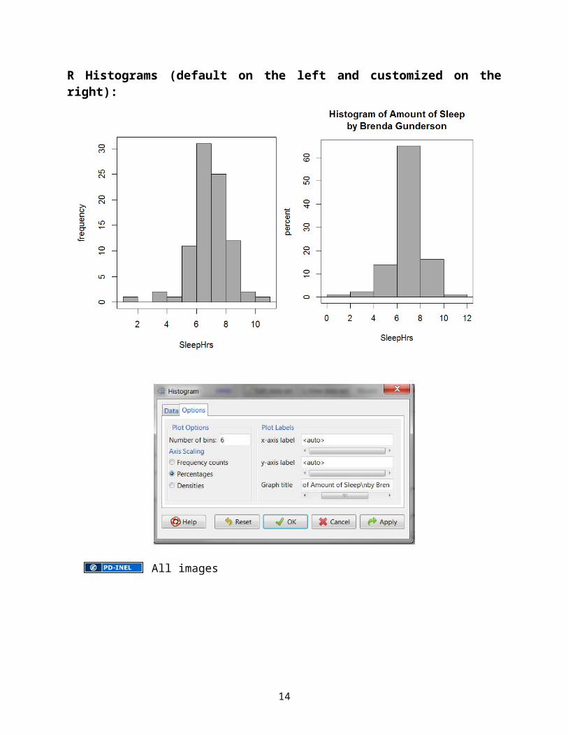
R Histograms (default on the left and customized on the right):

All images

10

Describe the distribution for SLEEP HOURS:

How to interpret? Look for Overall Pattern

Three summary characteristics of the overall distribution of the data …Shape (approximately symmetric, skewed, bell-shaped, uniform)

Location (center, average)

Spread (variability)

Look for deviations from Overall PatternOutliers = a data point that is not consistent with the bulk of the data. Outliers should not be discarded without justification.

What if … you had some data and you made a histogram of it and it looked like this…

What would it tell you? Response

Count

11

Other comments – NO SPACE BETWEEN BARS! Unless there are no observations in that interval. How Many Classes? Use your judgment: generally somewhere between 6 and 15

intervals. Better to use relative frequencies on the y axis when comparing two or more sets of

observations. Software has defaults and many options to modify settings.

One More Example:

A study was conducted in Detroit, Michigan to find out the number of hours children aged 8 to 12 years spent watching television on a typical day.

A listing of all households in a certain housing area having children aged 8 to 12 years was first constructed. Out of the 100 households in this listing, a random sample of 20 households was selected and all children aged 8 to 12 years in the selected households were interviewed.

The following histogram was obtained for all the children aged 8 to 12 years interviewed.

a. Complete the sentence: Based on this histogram, the distribution of number of hours spent watching TV is unimodal,

with a slight skewness to the __________.

b. Assuming that all children interviewed are represented in the histogram, what is the total number of children interviewed?

c. What proportion of children spent 2 hours or less watching television?

d. Can you determine the maximum number of hours spent watching television by one of the interviewed children? If so, report it. If not, explain why not.

0 1 2 3 4 5Number of hours watching TV

0

2

4

6

8

10

12

Freq

uenc

y

12

Numerical Summaries of Quantitative VariablesWe have discussed some interesting features of a quantitative data set and learned how to look for them in pictures (graphs). Section 2.5 focuses on numerical summaries of the center and the spread of the distribution (appropriate for quantitative data only).

Notation for a generic raw set of data: x1, x 2, x 3, …, x n where n = # items in the data set or sample size

Describing the Location or Center of a Data SetTwo basic measures of location or center:

Mean -- the numerical average valueWe represent the mean of a sample (called a statistic) by …

x=x1+x2+¿⋅¿+xn

n=∑ x in

Median -- the middle value when data arranged from smallest to largest.

Try It! French FriesWeight measurements for 16 small orders of French fries (in grams).

78 72 69 81 63 67 65 7579 74 71 83 71 79 80 69

What should we do with data first? Graph it!

Based on our histogram, the distribution of weight is unimodal and approximately symmetric, so computing numerical summaries is reasonable. The weights (in grams) range from the 60’s to the lower 80’s, centered around the lower 70’s, with no apparent outliers.

13

1. Compute the mean weight.

2. Compute the median weight.Ordered: 63, 65, 67, 69, 69, 71, 71, 72, 74, 75, 78, 79, 79, 80, 81, 83

3. What if the smallest weight was incorrectly entered as 3 grams instead of 63 grams?

Note: The mean is to extreme observations.

The median is to extreme observations.

Most graphical displays would have detected such an outlying value.

Some Pictures: Mean versus Median

14

Describing Spread: Range and Interquartile Range

Midterms are returned and the “average” was reported as 76 out of 100. You received a score of 88. How should you feel?

Often what is missing when the “average” of something is reported, is a corresponding measure of spread or variability. Here we discuss various measures of variation, each useful in some situations, each with some limitations.

Range: Measures the spread over 100% of the data. Range = High value – Low value = Maximum – Minimum

Percentiles: The pth percentile is the value such that p% of the observations fall at or below that value.

Some Common percentiles:Median: 50th percentileFirst quartile: 25th percentileThird quartile: 75th percentile

Five Number Summary: Variable Name and Units

(n = number of observations)Median M

Quartiles Q1 Q3Extremes Min Max

Provides a quick overview of the data values and information about the center and spread. Divides the data set into approximate quarters.

Interquartile Range: Measures the spread over the middle 50% of the data. IQR = Q3 – Q1

Try it! French Fries DataOrdered: 63, 65, 67, 69, 69, 71, 71, 72, 74, 75, 78, 79, 79, 80, 81, 83

Find the five-number summary:Weight of Fries (in grams)

(n = 16 orders)Median

QuartilesExtremes

Range: IQR:

15

And confirming these values using R we have:

> numSummary(FrenchFries[,"Weight"], statistics=c("mean", "sd", "IQR", + "quantiles"), quantiles=c(0,.25,.5,.75,1)) mean sd IQR 0% 25% 50% 75% 100% n 73.5 6.0663 10 63 69 73 79 83 16Example: Test ScoresThe five-number summary for the distribution of test scores for a very large math class is provided below:

Test Score (points)(n = 1200 students)

Median 58Quartiles 46 78Extremes 34 95

1. What is the test score interval containing approximately the lowest ¼ of the students?

2. Suppose you scored a 46 on the test. What can you say about the percentage of students who scored higher than you?

3. Suppose you scored a 50 on the test. What can you say about the percentage of students who scored higher than you?

4. If the top 25% of the students received an A on the test, based on this summary, what was the minimum score needed to get an A on the test?

BoxplotsA boxplot is a graphical representation of the five-number summary.Steps: Label an axis with values to cover the minimum and

maximum of the data. Make a box with ends at the quartiles Q1 and Q3. Draw a line in the box at the median M. Check for possible outliers using the 1.5*IQR rule

and if any, plot them individually. Extend lines from end of box to smallest and largest

observations that are not possible outliers.

Note: Possible outliers are observations that are more than 1.5*IQR outside the quartiles, that is, observations that are below Q1 - 1.5*IQR or observations that are above Q3 + 1.5*IQR.

16

Try it! French Fries DataOrdered: 63, 65, 67, 69, 69, 71, 71, 72, 74, 75, 78, 79, 79, 80, 81, 83

The five-number summary: Weight of Fries (in grams)

(n = 16 orders)

Median 73

Quartiles 69 79

Extremes 63 83

From the boxplot shown, we see there are no points plotted separately, so there are no outliers by the 1.5(IQR) rule.

Verify there are no outliers using this rule.

IQR = 79 – 69 = 10 grams

1.5*IQR = 1.5 (10) = 15 grams

Lower boundary (fence) = Q1 - 1.5*IQR =

Are there any observations that fall below this lower boundary?

Upper boundary (fence) = Q3 + 1.5*IQR =

Are there any observations that fall above this upper boundary?

17

What if … the largest weight of 83 grams was actually 95 grams?

Ordered: 63, 65, 67, 69, 69, 71, 71, 72, 74, 75, 78, 79, 79, 80, 81, 95

Then the five number summary would be:

Weight of Fries (in grams)(n = 12 orders)

Median 73Quartiles 69 79Extremes 63

The IQR and 1.5*IQR would be the same, so the “boundaries” for checking for possible outliers are again 54 and 94.

Now we would have one potential high outlier, the maximum value of 95.

The modified boxplot when we have this one outlier is shown.

Why is the line extending out on the top side now drawn out to just 81?

Notes on Boxplots: Side-by-side boxplots are good for ...

Watch out - points plotted individually are ...

Can't confirm ....

When reading values from a graph show what you are doing (so appropriate credit can be given on exam/quiz).

18

Try It: Side-by-side boxplotsA random sample of 100 parents of grade-school children were recently interviewed regarding the breakfast habits in their family. One question asked was if their children take the time to eat a breakfast (recorded as breakfast status – Yes or No). The grades of the children in some core classes (e.g. reading, writing, math) were also recorded and a standardized grade score (on a 10-point scale) was computed for each child. Side-by-side boxplots of the children’s standardized grade scores are provided.

a. What is (approx) the lowest grade scored by a child who does have breakfast?

___________ points

b. Complete the following sentence:

Among the children who did not eat breakfast,

25% had a grade score of at least _______________ points.

c. Consider the following statement: The symmetry in the boxplot for the children not eating breakfast implies that the distribution for the grade scores of such students is bell-shaped.

True or False?

Features of Bell-Shaped DistributionsWe have already described the distribution of our french fries weight data as being unimodal and somewhat symmetric. If we were to draw a curve to smooth out the tops of the bars of the histogram, it would resemble the shape of a bell, and thus could be called bell-shaped.

One fairly common distribution of measurements with this shape has a special name, called a normal distribution or normal curve. We will see normal curves in more detail when we study random variables. When a distribution is somewhat bell-shaped (unimodal, indicating a fairly homogeneous set of measurements), a useful measure of spread is called the standard deviation. In fact, the mean and the standard deviation are two summary measures that completely specify a normal curve.

Do you have breakfast?

YesNo

Gra

des

11

10

9

8

7

6

5

4

3

19

Describing Spread with Standard Deviation When the mean is used to measure center, the most common measure of spread is the standard deviation. The standard deviation is a measure of the spread of the observations from the mean. We will refer to it as a kind of “average distance” of the observations from the mean. But it actually is the square root of the average of the squared deviations of the observations from the mean. Since that is a bit cumbersome, we like to think of the standard deviation as “roughly, the average distance the observations fall from the mean.” Here is a quick look at the formula for the stand deviation when the data are a sample from a larger population:

s = sample standard deviation =

Note: The squared standard deviation, denoted by s2, is called the variance. We emphasize the standard deviation since it is in the original units.

Example: Consider this sample of n = 5 scores: 94, 97, 99, 103, 107. The sample mean is 100 points. Let’s measure their spread by considering how much each score deviates from the mean. Then consider the “average of these deviations”.

How the calculations are done:

x x – 100 (x – 100)2 Calculations1. x = 500/5 = 100 (used in columns 2 & 3)2. Variance: s2 = 104/(5-1) = 263. Standard deviation: s = √(26) = 5.1

Note # of deserved decimals used for s.

94 -6 3697 -3 999 -1 1

103 3 9107 7 49500 0 104 Sums (or totals) of the columns

90 95 100 105 110

Deviation from mean = 107 – 100 = 7

x x x x x

20

Try it! French Fries DataWeight measurements for 16 small orders of French fries (in grams).

78 72 69 81 63 67 65 7579 74 71 83 71 79 80 69

The mean was computed earlier to be 73.5. Find the standard deviation for this data.

s =

Not much fun to do it by hand, but not too bad for a small number of observations. In general, we will have a calculator or computer do it for us.

Interpretation:

The weights of small orders of french fries are roughly

________________away from their mean weight of , on average.

OR

On average, the weights of small orders of french fries vary by about ___

from their mean weight of .

Notes about the standard deviation: s = 0 means ...

Like the mean, s is ...

So use the mean and standard deviation for________________________________________.

The five-number summary is better for .

21

Technical Note about difference between population and sample:Datasets are commonly treated as if they represent a sample from a larger population. A numerical summary based on a sample is called a statistic. The sample mean and sample standard deviation are two such statistics. However, if you have all measurements for an entire population, then a numerical summary would be referred to as a parameter.

The symbols for the mean and standard deviation for a population are different, and the formula for the standard deviation is also slightly different. A population mean is represented by the Greek letter (“mu”), and a population standard deviation is represented by the Greek letter (“sigma”). The formula for the population standard deviation is below.

You will see more about the distinction between statistics and parameters in the next chapter and beyond.

Population standard deviation: =√∑ ( x i−μ )2

N where N is the size of the population.

Empirical RuleFor bell-shaped curves, approximately…

68% of the values fall within 1 standard deviation of the mean in either direction.

95% of the values fall within 2 standard deviations of the mean in either direction.

99.7% of the values fall within 3 standard deviations of the mean in either direction.

22

Try It! Amount of Sleep

The typical amount of sleep per night for college students has a bell-shaped distribution with a mean of 7 hours and a standard deviation of 1.7 hours.

About 68% of college students typically sleep between ________ and _______ hours per night.

Verify the values below that complete the sentences. About 95% of college students typically sleep between 3.6 and 10.4 hours per night. About 99.7% of college students typically sleep between 1.9 and 12.1 hours per night.

Draw a picture of the distribution showing the mean and intervals based on the empirical rule.

Suppose last night you slept 11 hours. How many standard deviations from the mean are you?

Suppose last night you slept only 5 hours. How many standard deviations from the mean are you?

The standard deviation is a useful “yardstick” for measuring how far an individual value falls from the mean. The standardized score or z-score is the distance between the observed value and the mean, measured in terms of number of standard deviations. Values that are above the mean have positive z-scores, and values that are below the mean have negative z-scores.

Standardized score or z-score:

23

Try It! Scores on a Final ExamScores on the final in a course have approximately a bell-shaped distribution. The mean score was 70 points and the standard deviation was 10 points.

Suppose Rob, one of the students, had a score that was 2 standard deviations above the mean. What was Rob’s score?

What can you say about the proportion of students who scored higher than Rob?

Sketching a picture may help.

Summary of Graphical Tools in Stat 350

350 Graphical Tools

Histo-gram

ScatterPlotsBoxplotsTime

PlotsQ-Q Plots

Freq. Tables

Pie Charts

BarCharts

QuantitativeVariables

Categorical Variables

Additional Notes

Summary Tools

24

A place to … jot down questions you may have and ask during office hours, take a few extra notes, write out an extra problem or summary completed in lecture, create your own summary about these

concepts.

25

Stat 250 Gunderson Lecture Notes2: Sampling, Surveys and Gathering Useful Data

Do not put faith in what statistics say until you have carefully considered what they do not say. -- William W. Watt

So far we have mainly studied how to summarize data - exploratory data analysis - with graphs and numbers. The knowledge of how the data were generated is one of the key ingredients for translating data intelligently. We will next discuss sampling, how to conduct surveys, how to make sure they are representative, and what can go wrong.

Collecting and Using Sample Data WiselyThere are two main types of statistical techniques that can be applied to data.

Definitions:Descriptive Statistics: Describing data using numerical summaries (such as the mean, IQR, etc.) and graphical summaries (such as histograms, bar charts, etc.).

Inferential Statistics: Using sample information to make conclusions about a larger group of items/individuals than just those in the sample.

In most statistical studies, the objective is to use a small group of units (the sample) to make an inference (a decision or judgment) about a larger group (the population).

Definitions:Population: The entire group of items/individuals that we want information about, about which inferences are to be made.Sample: The smaller group, the part of the population we actually examine in order to gather information.Variable: The characteristic of the items or individuals that we want to learn about.

One way to view these terms is through a Basket Model:

26

Fundamental Rule for Using Data for Inference:Available data can be used to make inferences about a much larger group if the data can be considered to be representative with regard to the question(s) of interest.

From Utts, Jessica M. and Robert F. Heckard. Mind on Statistics, Fourth Edition. 2012. Used with permission.

One principal way to guarantee that sample data represents a larger population is to use a (simple) random sample.

Try It! Fundamental Rule? For each situation explain whether or not the Fundamental Rule holds.

a. Research Question: Do a majority of adults in state support lowering the drinking age to 19?Available Data: Opinions on whether or not the legal drinking age should be lowered to 19 years old, collected from a random sample of 1000 adults in the state.

b. Research Question: Do a majority of adults in state support lowering the drinking age to 19?Available Data: Opinions on whether or not the legal drinking age should be lowered to 19 years old, collected from a random sample of parents of high school students in the state.

c. Available Data: Pulse rates for smokers and nonsmokers in a large stats class at a major university.Research Question: Do college-age smokers have higher pulse rates than college-age nonsmokers?

Sample versus CensusWhy can’t we learn about a population by just taking a census (measure every item in the population)? Takes too long, costs too much, measuring destroys the item. So, we often rely on a special type of statistical study called a sample survey, in which a subgroup of a large population is questioned on a set of topics.

Sample surveys are often used to estimate the proportion or percentage of people who have a certain trait or opinion. If you use proper methods to sample 1500 people from a population of many millions, you can almost certainly gauge the percentage of the entire population who have a certain trait or opinion to within 3%. The tricky part is that you have to use a proper sampling method.

27

Bias: How Surveys Can Go WrongWhile it is unlikely that the sample value will equal the population value exactly, we do want our surveys to be unbiased. Results based on a survey are biased if the method used to obtain those results would consistently produce values that are either too high or too low.

Selection bias occurs if the method for selecting the participants produces a sample that does not represent the population of interest.

Nonparticipation bias (nonresponse bias) occurs when a representative sample is chosen for a survey, but a subset cannot be contacted or does not respond.

Biased response or response bias occurs when participants respond differently from how they truly feel. The way questions are worded, the way the interviewer behaves, as well as many other factors might lead an individual to provide false information.From Utts, Jessica M. and Robert F. Heckard. Mind on Statistics, Fourth Edition. 2012. Used with permission.

Try It! Type of Bias Which type of bias do you think would be introduced if …a. A magazine sends a survey to a random sample of its subscribers asking them if they would

like the frequency of publication reduced from biweekly to monthly, or would prefer that it remain the same.

b. A random sample of registered voters is contacted by phone and asked whether or not they are going to vote in the upcoming presidential election.

Margin of Error, Confidence Intervals, and Sample SizeSample surveys are often used to estimate the proportion or percentage of all people who have a certain trait or opinion (p ). Newspapers and magazines routinely survey only one or two thousand people to determine public opinion on current topics of interest.

When a survey is used to find a proportion based on a sample ( p ) of only a few thousand individuals, one question is how close that proportion comes to the truth for the entire population. This measure of accuracy in sample surveys is a number called the margin of error.

The margin of error provides an upper limit on the amount by which the sample proportion p is expected to differ from the true population proportion p , and this upper limit holds for at least 95% of all random samples. To express results in terms of percents instead of proportions, simply multiply everything by 100.

28

Conservative (approximate 95%) Margin of Error = 1√n where n is the sample size.

We will see where this formula for the conservative margin of error comes from when we discuss in more detail confidence intervals for a population proportion. For now we will consider an approximate 95% confidence interval for a population proportion to be given by:

Approximate 95% Confidence Interval for p:

sample proportion 1√n or expressed as p

1√n

Try It! School QualityA survey of 1,250 adults was conducted to determine How Americans Grade the School System. One question: In general, how would you rate the quality of American public schools?

Frequency Distribution of School Quality ResponsesExcellent 462

Pretty Good 288Only Fair 225

Poor 225Not Sure 50

a. What type of response variable is school quality?

b. What graph is appropriate to summarize the distribution of this variable?

c. What proportion of sampled adults rated the quality of public schools as excellent?

d. What is the conservative 95% margin of error for this survey?

e. Give an approximate 95% (conservative) confidence interval for the population proportion of all adults that rate the quality of public schools as excellent.

Interpretation Note: Does the interval in part (e) of 34.2% to 39.8% actually contain the population proportion of all adults that rate the quality of public schools as excellent?

It either does or it doesn’t, but we don’t know because we don’t know the value of the population proportion. (And if we did know the value of p then we would not have taken a sample of 1250 adults to try to estimate it).

The 95% confidence level tells us that in the long run, this procedure will produce intervals that contain the unknown population proportion p about 95% of the time.

29

f. Bonus #1: What (approximate) sample size would be necessary to have a (conservative 95%) margin of error of 2%?

g. Bonus #2: How does the margin of error for a sample of size 1000 from a population of 30,000 compare to the margin of error for a sample of size 1000 from a population of 100,000?

Sampling MethodsThere are good sampling designs and poor ones.

Poor: volunteer, self-selected, convenience samples, often biased in favor of some items over others.

Good: involve random selection, giving all items a non-zero change of being selected.

Most of our inference methods require the data be considered a …

______________________ ___________________________.

This implies that the responses are to be independent and identically distributed (iid). We will make this more formal later after probability, but here are the basic ideas between these two properties.

Independent =the response you will obtain from one individual the response you will get from another individual.

Identically distributed = all of the responses .

Many sampling designs are discussed in your text (SRS, stratified, cluster, etc). We will not cover the details of these various methods, nor work with a random number table. However, we will expect you to think about whether the data available can be considered a random sample, based on the fundamental rule for using data for inference.

We will also discuss various graphs that sometimes can be used for checking assumptions, one of which is a time plot for assessing the identically distributed property of a random sample (if the data are collected over time).

Difficulties and Disasters in SamplingThis section presents some of the problems that can arise even when a sampling plan has been well designed. It talks about sampling from the wrong population, relying on volunteer response, and meaningless polls.

30

How to Ask Survey Questions The wording and presentation of questions can significantly influence the results of a survey. Here is one example of a pitfall that is a possible source of response bias in a survey.

Asking the Uninformed People do not like to admit that they don’t know what you are talking about when you ask them a question. Crossen (1994, p. 24) gives an example: “When the American Jewish Committee studied Americans’ attitudes toward various ethnic groups, almost 30% of the respondents had an opinion about the fictional Wisians, rating them in social standing above a half-dozen other real groups, including Mexicans, Vietnamese and African blacks.”

Try It! Consider the following two questions:1. Considering that research has shown that exposure to cigarette smoke is harmful,

do you think smoking should be allowed in all public restaurants or not?2. Considering it is not against the law to smoke, do you agree that smoking should be

allowed in all public restaurants?”

Here are the two results: 30% favored banning smoking 70% favored banning smoking

Which question (1 or 2) produced the 30%, which the 70%?A more neutral and unbiased question might be: Do you believe smoking should or should not be allowed in all public restaurants?

Types of StudiesTwo Basic Types of Research Studies: Observational or Experimental

Definitions:Observational Studies: The researchers simply observe or measure the participants (about opinions, behaviors, or outcomes) and do not assign any treatments or conditions. Participants are not asked to do anything differently.

Experiments: The researchers manipulate something and measure the effect of the manipulation on some outcome of interest. Often participants are randomly assigned to the various conditions or treatments.

Most studies, observational or experimental, are interested in learning of the effect of one variable (explanatory variable) on another variable (response or outcome variable).

A confounding variable is a variable that both affects the response variable and also is related to the explanatory variable. The effect of a confounding variable on the response variable cannot be separated from the effect of the explanatory variable.

Confounding variables are especially a problem in observational studies. Randomized experiments help control the influence of confounding variables.

31

Try It! Student’s Health StudyA researcher at the University of Michigan believes that the number of times a student visits the Student Health Center (SHC) is strongly correlated with the student’s type of diet and their amount of weekly exercise. The researcher selected a simple random sample of 100 students from a total of 3,568 students that visited SHC last month and first recorded the number of visits made to the SHC for each selected student over the previous 6 months. After recording the number of visits, he looked into their records and classified each student according to the type of diet (Home-Cooked/Fast Food) and the amount of exercise (None/Twice a Week/Everyday).

a. Is this an observational study or a randomized experiment?

b. What are the explanatory and response variables?

Try It! External Clues StudyA study examined how external clues influence student performance. Undergraduate students were randomly assigned to one of four different forms for their midterm exam. Form 1 was printed on blue paper and contained difficult questions, while Form 2 was also printed on blue paper but contained simple questions. Form 3 was printed on red paper, with difficult questions, and Form 4 was printed on red paper with simple questions. The researchers were interested in the impact that color and type of question had on exam score (out of 100 points).

a. This research is based on: an observational study a randomized experiment

b. Complete the following statements by circling the appropriate answer.i. The color of the paper is a(n) response explanatory variable

and its type is (circle one) categorical quantitative.

ii. The exam score is a(n) response explanatory variable

and its type is (circle one) categorical quantitative.

c. Fill in the blank. Suppose students in the “blue paper” group were mostly upper-classmen and the students in the “red paper” group were mostly first and second-year students.

The variable “class rank” is an example of a(n) variable.

A Little More about Studies:Hawthorne Effect, Placebo Effect, Randomized Studies, Control Groups, and Blinding

The Hawthorne Effect – In early studies from 1924-1932 at the Hawthorne Works (a Western Electric factory outside Chicago), investigators studied how various changes to the production process could increase production. In general, they observed that no matter what “production changes” were adapted, overall production levels increased. However, when the observations and recordings stopped, then production levels slumped back to what they had been before. Simply said, when someone observes and records a particular behavior, that behavior may improve during the observation period,

32

but then return to usual behavior levels thereafter. To understand more about the phenomena called the Hawthorne effect see the first few pages of: http://en.wikipedia.org/wiki/Hawthorne_effect

The Placebo Effect – The placebo effect refers to the phenomenon in which some people experience some type of benefit after the administration of a placebo (a substance with no known medical benefit, e.g., a sugar pill or a saline solution). In short, a placebo is a fake treatment that in some cases can produce a real and positive response. For more info see: http://psychology.about.com/od/f/placebo-effect.htm

A Randomized Study (or Experiment) – These experiments involve the comparison of at least two treatments or methods (say Treatment A versus Treatment B). A group of study participants (or subjects) is randomized to receive either Treatment A or Treatment B using a “randomization schedule” which may involve a series of “random digits” or flips of a coin. The randomization is usually 1:1, that is, an equal number of subjects per treatment, or balanced; although some studies have been conducted using a 2:1 randomization where twice as many subjects are assigned to one treatment compared to the other. To learn more, see “Explorable Psychology Experiments” website: https://explorable.com/randomization

Blinding – In an experiment where Treatment A is compared to Treatment B, it is quite common to stipulate that the design be “single blinded”, that is, the subjects are completely unaware of which treatment they are receiving. This blinding is found in pharmaceutical studies in which the pills or capsules appear exactly the same.

A study is said to be “double blinded” if not only are the subjects receiving the treatment ‘blinded’, but also the study personnel who recruit the subjects or who guide the subjects through the various procedures are also “blinded” as to actual treatment the subject received. This is especially true for the study personnel who gather and record the data, especially the measurements regarding how each subject is responding to treatment. Such study personnel having knowledge of which patients are given the various treatments has the potential to bias the various efficacy measurements.

Pharmaceutical companies quite often insist on a “triple-blind” study design in which personnel at the company itself also remain unaware to the treatment assignment of the subjects until all the data has been obtained and cleaned (carefully examined to insure the consistency and correctness of each value in the database).

Blinding can help reduce the potential for bias in studies. https://explorable.com/randomization

A Placebo-Controlled Study – Studies that compare the response of an experimental treatment with a placebo are called placebo-controlled studies.

An Active-Controlled Study – An active control is a treatment that has already been shown to be an efficacious product by several previous investigations and is so recognized by the medical community. Studies that compare the response of an experimental treatment with an active-control are called active-controlled studies. For more information Trial Design in http://en.wikipedia.org/wiki/clinical-trial

33

Where are we going? We have a population (a basket) that we cannot examine but we want to learn something

about it - so we will take a sample - preferably it will be a random sample. We will use the sample to estimate the things we wanted to know about the population -

we will use the sample results to test theories about the population and make some decisions.

Since the sample is just a part of the population there will be some uncertainty about the estimates and decisions we make. To measure and quantify that uncertainty we turn to PROBABILITY!

34

Additional NotesA place to … jot down questions you may have and ask during office hours, take a few extra notes, write out an extra problem or summary completed in lecture, create your own summary about these

concepts.

35

Stat 250 Gunderson Lecture Notes3: Probability

Chance favors prepared minds. -- Louis Pasteur

Many decisions that we make involve uncertainty and the evaluation of probabilities.

Interpretations of ProbabilityExample: Roll a fair die possible outcomes = { }

Before you roll the die do you know which one will occur?What is the probability that the outcome will be a ‘4’? __________ Why?

A few ways to think about PROBABILITY:

(1) Personal or Subjective Probability P(A) = the degree to which a given individual believes that the event A will happen.

(2) Long term relative frequency P(A) = proportion of times ‘A’ occurs if the random experiment (circumstance) is repeated many, many times.

(3) Basket Model P(A) = proportion of balls in the basket that have an ‘A’ on them.

10 balls in the basket: 3 blue and 7 whiteOne ball will be selected at random.

What is P(blue)? ______________

Note: A probability statement IS NOT a statement about .

It IS a statement about .

Discover Basic Rules for Finding Probability through an ExampleThere is a lot you can learn about probability. One basic rule to always keep in mind is that the probability of any outcome is always between 0 and 1. Now, there are entire courses devoted just to studying probability. But this is a Statistics class. So rather than start with a list of

36

definitions and formulas for finding probabilities, let’s just do it through an example so you can see what ideas about probability we need to know for doing statistics.Example: Shopping OnlineMany Internet users shop online. Consider a population of 1000 customers that shopped online at a particular website during the past holiday season and their results regarding whether or not they were satisfied with the experience and whether or not they received the products on time. These results are summarized below in table form. Using the idea of probability as a proportion, try answering the following questions.

On Time Not On Time TotalSatisfied 800 20 820Not Satisfied 80 100 180Total 880 120 1000

a. What is the probability that a randomly selected customer was satisfied with the experience?

b. What is the probability that a randomly selected customer was not satisfied with the experience?

c. What is the probability that a randomly selected customer was both satisfied and received the product on time?

d. What is the probability that a randomly selected customer was either satisfied or received the product on time?

e. Given that a customer did receive the product on time, what is the probability that the customer was satisfied with the experience?

f. Given that a customer did not receive the product on time, what is the probability that the customer was satisfied with the experience?

37

Note: We stated the above 1000 customers represented a population. If results were based on a sample that is representative of a larger population, then the observed sample proportions would be used as approximate probabilities for a randomly selected person from the larger population.

38

Great job! You just computed probabilities using many of the basic probability rules or formulas summarized below and also found in your textbook.

Complement rule P( AC )=1−P( A )

Addition rule P( A or B )=P( A )+P(B )−P( A and B )

Multiplication rule P( A and B )=P( A )P(B|A )

Conditional Probability P( A|B )=

P( A and B )P(B )

You did not need the formulas themselves but instead used intuition and approaching it as some type of proportion. Let’s see how your intuition and the above formulas really do connect.

In part b you found the probability of “NOT being satisfied”, which is the complement of the event “being satisfied”, so the answer to part b is the complement of the probability you found in part a.

In part c, there was a key word of “AND” in the question being asked. The “AND” is just the intersection, or the overlapping part; the outcomes that are in common. The picture at the right show an intersection between the event A and B. In a table, the counts that are in the middle are the “AND” counts; there were 800 (out of the 1000 customers) that were both satisfied AND received the product on time. There is a multiplication formula above for finding probabilities of the AND or intersection of two events, but we did not even need to apply it; as a table presentation of counts provides “AND” counts directly.

In part d, there was a key word of “OR” in the question being asked. The “OR” is union, the outcomes that are in either one or the other (including those that are in both). The picture at the right show an union between the event A and B. Notice that if you start with all of the outcomes that are in A and then add all of the outcomes that are in B, you have double counted the outcomes that are in the overlap. So the addition formula above shows you need to subtract off the intersecting probability once to correct for the double counting. From the table, you could either add up the separate counts of 800 + 20 + 80; or start with the 820 that were satisfied and add the 880 that received it on time and then subtract the 800

39

that were in both sets; to get the 900 in all that were either satisfied or received the product on time.

40

Finally, parts e and f were both conditional probabilities. In part e you were first told to consider only the 880 customers that received the product on time, and out of these find the probability (or proportion) that were satisfied. There were 800 out of the 880 that were satisfied. The picture below shows the idea of a conditional probability formula above for P(A | B), read as the probability of A given B has occurred. If we know B has occurred, then only look at those items in the event B. The event B, shaded at the right, is our new ‘base’ (and thus is in

the denominator of the formula). Now out of those items in B, we want to find the probability of A. The only items in A that are on the set B are those in the overlap or intersection. So the conditional formula above shows you count up those in the “A and B” and divide it by the base of “B”.

Try It! Go back to parts a to f and add the corresponding shorthand probability notation of what you actually found; e.g. P(satisfied), P(satisfied | on time) next to each answer.

Now there are a couple of useful situations that can make computing probabilities easier.

Definition: Two events A, B are Mutually Exclusive (or Disjoint) if ... they do not contain any of the same outcomes. So their intersection is empty.

We can easily picture disjoint events because the definition is a property about the sets themselves.

If A, B are disjoint, then P(A and B) = 0. If there are no items in the overlapping part, then man of the probability results will simplify. For example, the additional rule for disjoint events P(A or B) = P(A) + P(B).

41

Another important situation in statistics occurs when the two events turn out to be independent.

Definition: Two events A, B are said to be independent if knowing that one will occur (or has occurred) does not change the probability that the other occurs. In notation this can be expressed as P(A|B) = P(A).

This expression P(A|B) = P(A) tells us that knowing the event B occurred does not change the probability of the event A happening.

Now it works the other way around too, if A and B are independent events, then P(B|A) = P(B).

As a result of this independence definition, we could show that the multiplication rule for independent events reduces to P(A and B) = P(A)P(B).

Finally, this rule can also be extended. If three events A, B, C are all independent then P(A and B and C) = P(A)P(B)P(C).

So let’s apply these two new concepts to our online shopping example.

Back to the Shopping Online Example

Below are results for a population of 1000 customers that shopped online at a particular website during the past holiday season. Recorded was whether or not they were satisfied with the experience and whether or not they received the products on time.

On Time Not On Time TotalSatisfied 800 20 820Not Satisfied 80 100 180Total 880 120 1000

g. Are being satisfied with the experience and receiving the product on time mutually exclusive (disjoint)? Provide support for your answer.

h. Are being satisfied with the experience and receiving the product on time statistically independent? Provide support for your answer.

Hint: go back and compare your answers to parts a, e, and f.

42

Try It! Elderly People Suppose that in a certain country, 10% of the elderly people have diabetes. It is also known that 30% of the elderly people are living below poverty level and 5% of the elderly population falls into both of these categories.

At the right is a diagram for these events. Do the probabilities make sense to you?

a. What is the probability that a randomly selected elderly person is not diabetic?

b. What is the probability that a randomly selected elderly person is either diabetic or living below poverty level?

c. Given a randomly selected elderly person is living below poverty level, what is the probability that he or she has diabetes?

d. Since knowing an elderly person lives below the poverty level (circle one)

DOES DOES NOT change the probability that they are diabetic, the two

events of living below the poverty level and being diabetic (circle one)

ARE ARE NOT independent.

diabetes below poverty

E l d e r l y P e o p l e

0.05 0.05 0.25

Neither diabetes nor below poverty

diabetes & below poverty 0.65

43

In the next example, you are not asked to determine if two events are independent, but rather put independence to use.

Try It! Blood TypeAbout 1/3 of all adults in the United States have type O+ blood. Suppose three adults will be randomly selected. Hint: randomly selected implies the results should be_______________________.

What is the probability that the first selected adult will have type O+ blood?

What is the probability that the second selected adult will have type O+ blood?

What is the probability that all three will have type O+ blood?

What is the probability that none of the three will have type O+ blood?

What is the probability that at least one will have type O+ blood?

Some final notes…I. Sampling with and without Replacement

Definitions:A sample is drawn with replacement if individuals are returned to the eligible pool for each selection. A sample is drawn without replacement if sampled individuals are not eligible for subsequent selection.

If sampling is done with replacement, the Extension of Rule 3b holds. If sampling is done without replacement, probability calculations can be more complicated because the probabilities of possible outcomes at any specific time in the sequence are conditional on previous outcomes.

If a sample is drawn from a very large population, the distinction between sampling with and without replacement becomes unimportant. In most polls, individuals are drawn without

44

replacement, but the analysis of the results is done as if they were drawn with replacement. The consequences of making this simplifying assumption are negligible.

II. Sometimes students confuse the mutually exclusive with independence.

Check the definitions. The definition for two events to be disjoint (mutually exclusive) was based on a SET

property. The definition for two events to be independent is based on a PROBABILITY property.

You need to check if these definitions hold when asked to assess if two events are disjoint, or if two events are independent.

Mutually Exclusive Independence

If two events are mutually exclusive then we know that P(A and B) = 0. This also implies that P(A|B) is equal to 0 (if the two events are disjoint and B did occur, then the chance of A occurring is 0).

So P(A|B) (which is 0) will not be equal to P(A) if the events are disjoint.

III. Probability rules summaryBelow is a summary of the key probability results you need to understand and be able to use.

Complement rule P( AC )=1−P( A )

Mutually Exclusive (disjoint) Events: The events A, B are disjoint if “A and B” is the empty set. Thus, P(A and B) = 0.

Addition Rule (general) P( A or B )=P( A )+P(B )−P( A and B )

If A, B are disjoint, we have P( A or B )=P( A )+P(B )

Conditional Probability (general) P( A|B )=

P( A and B )P(B )

Independent Events:

The events A, B are independent if P( A|B )=P (A )Equivalently, the events A, B are independent

if P( A and B )=P( A )P(B)

45

The Stats 250 formula card provides a more extensive list, but remember, you may not need them as you discovered in your first probability example with the online customers.

Additional NotesA place to … jot down questions you may have and ask during office hours, take a few extra notes, write out an extra problem or summary completed in lecture, create your own summary about these

concepts.

46

47

Stat 250 Gunderson Lecture Notes4: Random Variables

All models are wrong; some models are useful. -- George Box

Patterns make life easier to understand and decisions easier to make. Earlier we discussed the different types of data or variables and how to turn the data into useful information with graphs and numerical summaries. Having some notion of probability from the previous chapter, we can now view the variables as “random variables” – the numerical outcomes of a random circumstance. We will look at the pattern of the distribution of the values of a random variable and we will see how to use the pattern to find probabilities. These patterns will serve as models in our inference methods to come.

What is a Random Variable? Recall in our discussion on probability we started out with some random circumstance or experiment that gave rise to our set of all possible outcomes S. We developed some rules for calculating probabilities about various events. Often the events can be expressed in terms of a “random variable” taking on certain outcomes. Loosely, this random variable will represent the value of the variable or characteristic of interest, but before we look. Before we look, the value of the variable is not known and could be any of the possible values with various probabilities, hence the name of a “random” variable.

Definition: A random variable assigns a number to each outcome of a random circumstance, or, equivalently, a random variable assigns a number to each unit in a population.

We will consider two broad classes of random variables: discrete random variables and continuous random variables.

Definitions: A discrete random variable can take one of a countable list of distinct values. A continuous random variable can take any value in an interval or collection of intervals.

Try It! Discrete or ContinuousA car is selected at random from a used car dealership lot. For each of the following characteristics of the car, decide whether the characteristic is a continuous or a discrete random variable.a. Weight of the car (in pounds).

b. Number of seats (maximum passenger capacity).

c. Overall condition of car (1 = good, 2 = very good, 3 = excellent).

48

d. Length of car (in feet).

In statistics, we are interested in the distribution of a random variable and we will use the distribution to compute various probabilities. The probabilities we compute (for example, p-values in testing theories) will help us make reasonable decisions.

So just what is the distribution of a random variable? Loosely, it is a model that shows us what values are possible for that particular random variable and how often those values are expected to occur (i.e. their probabilities). The model can be expressed as a function, table, picture, depending on the type of variable it is.

We will first discuss discrete random variables and their models. We will work with the broad class of general discrete random variables and then focus on a particular family of discrete random variables called the Binomial. The Binomial random variable arises in situations where you are counting the number of successes that occur in a sample.

Next we look at properties for continuous random variables and spend more time studying the family of uniform random variables and normal random variables. Later in this class you will be introduced to more models for continuous random variables that are primarily used in statistical testing problems. Below is a summary of the types of random variables we will work with in this course.

Random Variable

Discrete Continuous

Binomial Uniform Normal More

to come

Technical Note: Sometimes a random variable fits the technical definition of a discrete random variable but it is more convenient to treat it, that is, model it, as if it were continuous. We will learn when it is reasonable to model a discrete binomial random variable as being approximately normal. Finally we will also learn how to model sums and differences of random variables.

Some general notes about random variables are: random variables will be denoted by capital letters (X, Y, Z); outcomes of random variables are represented with small letters ( x, y, z).

49

So when we express probabilities about the possible value of a random variable we use the capital letter. For example, the probability that a random variable takes on the value of 2 would be expressed as P(X = 2).

50

General Discrete Random VariablesA discrete random variable, X , is a random variable with a finite or countable number of possible outcomes. The probability notation your text uses for a Discrete Random Variable is given next:

Discrete Random Variable: X = the random variable.k = a number that the discrete random variable could assume. P(X = k) is the probability that the random variable X equals k.

The probability distribution function (pdf) for a discrete random variable X is a table or rule that assigns probabilities to the possible values of the X. One way to show the distribution is through a table that lists the possible values and their corresponding probabilities:

Value of X x1 x2 x3 …Probability p1 p2 p3 …

Two conditions that must apply to the probabilities for a discrete random variable are:Condition 1: The sum of all of the individual probabilities must equal 1.Condition 2: The individual probabilities must be between 0 and 1.

A probability histogram or better yet, a probability stick graph, can be used to display the distribution for a discrete random variable.

The x-axis represents the values or outcomes.The y-axis represents the probabilities of the values or outcomes.

The cumulative distribution function (cdf) for a discrete random variable X is a table or rule that provides the probabilities P(X k) for any real number k. Generally, the term cumulative probability refers to the probability that X is less than or equal to a particular value.

Try It! Psychology ExperimentA psychology experiment on the behavior of young children involves placing a child in a designated area with five different toys. Over a fixed time period various observations are made. One response measured is the number of toys the child plays with. Based on many results, the (partial) probability distribution below was determined for the discrete random variable X = number of toys played with by children (during a fixed time period).

X = # toys 0 1 2 3 4 5Probability 0.03 0.16 0.30 0.23 0.17

a. What is the missing probability P(X = 5)?

51

Psychology Experiment continuedX = # toys 0 1 2 3 4 5

Probability 0.03 0.16 0.30 0.23 0.17

b. Graph this discrete probability distribution function for X.

X

543210

Pro

babi

lity

.50

.45

.40

.35

.30

.25

.20

.15

.10

.05

0.00

c. What is the probability that a child will play with at least 3 toys?

d. Given the child has played with at least 3 toys, what is the probability that he/she will play with all 5 toys?

e. Finish the table below to provide the cumulative distribution function of X.X = # toys 0 1 2 3 4 5

Cum ProbabilityP(X k) 0.03 0.03+0.16

= 0.190.03+0.16+0.30

= 0.49

52

Expectations for Random VariablesJust as we moved from summarizing a set of data with a graph to numerical summaries, we next consider computing the mean and the standard deviation of a random variable. The mean can be viewed as the expected value over the long run (in many repetitions of the random circumstance) and the standard deviation can be viewed is approximately the average distance of the possible values of X from its mean.

Definition: The expected value of a random variable is the mean value of the variable X in the sample space, or population, of possible outcomes. Expected value, denoted by E(X), can also be interpreted as the mean value that would be obtained from an infinite number of observations on the random variable.

Motivation for the expected value formula …

Consider a population consisting of 100 families in a community. Suppose that 30 families have just 1 child, 50 families have 2 children, and 20 families have 3 children. What is the mean or average number of children per family for this population?

Definitions: Mean and standard deviation of a discrete random variableSuppose that X is a discrete random variable with possible values x1, x2, x3, … occurring with probabilities p1, p2, p3, …, then

the expected value (or mean) of X is given by = E(X) = ∑ x i pi

the variance of X is given by V(X) = = ∑ ( x i−μ )2 p i

and so the standard deviation of X is given by = √∑ ( xi−μ )2 piThe sums are taken over all possible values of the random variable X.

11

122

22 3

3 etc.2

2

Population of 100 families

Mean = (sum of all values)/100= [1(30) + 2(50) + 3(20)]/100= 1(30/100) + 2(50/100) + 3(20/100) = 1(0.30) + 2(0.50) + 3(0.20) = 1.9 children per family

Mean = Sum of (value x probability of that value)

53

Try It! Psychology ExperimentRecall the probability distribution for the discrete random variable X=number of toys played with by children.

X = # toys 0 1 2 3 4 5Probability 0.03 0.16 0.30 0.23 0.17 0.11

a. What is the expected number of toys played with?

Note: The expected value may not be a value that is ever expected on a single random outcome. Instead, it is the average over the long run.

b. What is the standard deviation for the number of toys played with?

c. Complete the interpretation of this standard deviation (in terms of an average distance):

On average, the number of toys played with vary by about ____________

from the mean number of toys played with of ___________.

Binomial Random VariablesAn important class of discrete random variables is called the Binomial Random Variables.

A binomial random variable is that it COUNTS the number of times a certain event occurs out of a particular number of observations or trials of a random experiment.

Examples of Binomial Random Variables: The number of girls in six independent births. The number of tall men (over 6 feet) in a random sample of 30 men from a large male population.

54

A binomial experiment is defined by the following conditions:1. There are n “trials”, n is determined in advance and is not a random value.2. There are two possible outcomes on each trial,

called “success” (S) and “failure” (F).3. The outcomes are independent from one trial to the next.4. The probability of a “success” remains the same from one trial to the next, and this

probability is denoted by p. The probability of a “failure” is 1 – p for every trial.

A binomial random variable is defined asX = number of successes in the n trials of a binomial experiment.

Try It! Are the Conditions Right for Binomial?a. Observe the sex of the next 50 children born at a local hospital.

X = number of girls

b. A ten-question quiz has five True-False questions and five multiple-choice questions, each with four possible choices. A student randomly picks an answer for every question.

X = number of answers that are correct.

c. Four students are randomly picked without replacement from large student body listing of 1000 women and 1000 men.

X = number of women among the four selected students.

What if the student body listing consisted only of 10 women and 10 men?

Rule of Thumb: population at least 10 times as large as the sample ok!

55

The Binomial FormulaWe will develop the formula together using our probability knowledge. Suppose that of the online shoppers for a particular website that start filling a shopping cart with items, 25% actually make a purchase (complete a transaction). We have a random sample of 10 such online shoppers.

If the stated rate is true, what is the probability that ...

... all 10 shoppers will actually make a purchase?

... none of the shoppers will make a purchase?

... just 1 shopper will make a purchase?

With only the basic probability knowledge, you just calculated three binomial probabilities that are based on the following formula.

The binomial distribution:Probability of exactly k successes in n trials …

P(X=k )=(nk ) pk (1− p)n−k

for k=0,1,2 ,. . ., n

56

where (nk )= n !

k !(n−k )! (this represents the # of ways to select k items from n)

57

Try it! The first part …

You can think of the computation of (nk ) in the following way …

Suppose you had n friends, how many ways could you invite k to dinner? The ones “at the ends” are easy to do without even using the formula or a calculator. Your calculator is likely to have this complete function or at least a factorial ! option. On many calculators this combinations function is found under the math probability menu and expressed as nCr.

1.(10

0 )=2.

(1010 )=

3.(10

1 )=4.

(109 )=

5.(10

2 )=

Try it! Finding Binomial ProbabilitiesRecall we have a random sample of n = 10 online shoppers from a large population of such shoppers and that p = 0.25 is the population proportion who actually make a purchase.a. What is the probability of selecting exactly one shopper who actually makes a purchase?

b. What is the probability of selecting exactly two shoppers who actually make a purchase?

c. What is the probability of selecting at least one shopper who actually makes a purchase?

d. How many shoppers in your random sample of size 10 would you expect to actually make a purchase?

58

In the previous question (part d), you just computed the mean of a binomial distribution.

If X has the binomial distribution Bin(n, p) thenMean of X is = E(X) = np

Standard Deviation of X, is = √np (1−p )

Try it! More Work with the Binomial Suppose that about 10% of Americans are left-handed. Let X represent the number of left-handed Americans in a random sample of 12 Americans.

Then X has a __________________________distribution (be as specific as you can).

Note that the mean or expected number of left-handed Americans in such a random sample would be = np = 12(0.10) = 1.2. The standard deviation (reflecting the variability in the results

from the mean across many such random samples) is = √np(1−p )=√12(0 . 10)(0 . 90 )= 1.04.

a. What is the probability that the sample contains 2 or fewer left-handed Americans?

b. Suppose a random sample of 120 Americans had been taken instead of just 12. So now X has a Binomial(n = 120, p = 0.10) model. The mean or expected number of left-handed Americans in a random sample of 120 will be = np = 120(0.10) = 12. The standard

deviation for the number of left-handed Americans will be √np(1−p )=√120(0 . 10)(0 . 90 )= 3.29.

So how might you try to find the probability that a random sample of 120 Americans would result in 20 or fewer left-handed Americans? Note that 2 out of n = 12 is 16.67% and that 20 out of n = 120 is also equal to 16.67%.

59

General Continuous Random Variables

A continuous random variable, X , takes on all possible values in an interval (or a collection of intervals). The way that we determine probabilities for continuous random variables differs in one important respect from how we determine probabilities for discrete random variables. For a discrete random variable, we can find the probability that the variable X exactly equals a specified value. We can’t do this for a continuous random variable. Instead, we are only able to find the probability that X could take on values in an interval. We do this by determining the corresponding area under a curve called the probability density function of the random variable.

We have already summarized the general shapes of distributions of a quantitative response that often arise with real data. The shape of a distribution was found by drawing a smooth curve that traces out the overall pattern that is displayed in a histogram. With a histogram, the area of each rectangle is proportional to the frequency or count for each class. The curve also provides a visual image of proportion through its area. If we could get the equation of this smoothed curve, we would have a simple and somewhat accurate summary of the distribution of the response.

The picture at the right shows a smoothed curve that is symmetric and bell shaped, even though the underlying histogram is only approximately symmetric. If the data came from a representative sample, the smooth curve could serve as a model, that is, as the probability distribution for the continuous response for the population.

So the probability distribution of a continuous random variable is described by a density curve. The probability of an event is the area under the curve for the values of X that make up the event.

The probability model for a continuous random variable assigns probabilities to intervals.

Definition: A curve (or function) is called a Probability Density Curve if:

1. It lies on or above the horizontal axis. 2. Total area under the curve is equal to 1.

KEY IDEA: AREA under a density curve over a range of values corresponds to the PROBABILITY that the random variable X takes on a value in that range.

60

Try It! Some Probability Density Curves

I. A density curve for modeling income for employed adults (in $1000s) for a city.

How would you use the above density curve to estimate the probability of a randomly selected employed adult from this city having an income between $30,000 and $40,000?

II. Consider the following curve:

30 50

a. Is this a density curve? Why?

b. If yes, find the probability of observing a response that is less than 35.

c. What does the value of 35 correspond to for this distribution?

1/20

61

Try it! Checkout time at a storeLet X be the checkout time at a store, which is a random variable that is uniformly distributed on values between 5 and 20 minutes. That is, X is U(5, 20).

a. What does the density look like? Sketch it and include a value on the y-axis.

X=time to check out (minutes)

20151050

Density

0 5 10 15 20

b. What is the probability a person will take more than 10 minutes to check out?

c. Given a person has already spent 10 minutes checking out, what is the probability they will take no more than 5 additional minutes to check out?

d. What is the expected time to check out at this store?

Definition: Mean of a continuous random variable.Expected Value or Mean = Balancing point of the density curve E(X) =(Sometimes one would need calculus/integration to find it -- integral instead of sums)

There are many density curves that can be used as models. Next we focus on an important family of densities called the NORMAL DISTRIBUTIONS.

62

Normal Random Variables We had our first introduction to normal random variables back in our summarizing data section as a special case of bell-shaped distributions. The family of normal distributions is very important because many variables have this shape and form approximately and many statistics that we use in our inference methods are based on sums or averages which generally have (approximately) a normal distribution.

A Normal Curve: Symmetric, bell-shaped, centered at the mean μ and its spread is determined by the standard deviation σ . In fact, the points of inflection on each side of the mean mark the values which are one standard deviation away from the mean.

Notation: If a population of measurements follows a normal curve, and if X is the measurement for a randomly selected individual from the population, then X is said to be a normal random variable. X is also said to have a normal distribution. Any normal random variable can be completely characterized by its mean and its standard deviation.

The variable X is normally distributed with mean μ and standard deviation σ is denoted by:

A N(50,10) curve is sketched below. Add a N(80,5) curve to this picture. Keep in mind the features of the empirical rule (68-95-99.7) which applies to a normal curve.

63

Standardized Scores:A normal distribution is indexed by its population mean μ , and its population standard deviation σ , and denoted by N ( μ ,σ ). Recall that the standard deviation is a useful “yardstick” for measuring how far an individual value falls from the mean. The standardized score or z-score is the distance between the observed value and the mean, measured in terms of number of standard deviations. Values that are above the mean have positive z-scores, and values that are below the mean have negative z-scores.

Standardized score or z-score:

Finding Probabilities for z-Scores:Standard scores play a role in how we will find areas (and thus probabilities) under a normal curve. We simply convert the endpoints of the interval of interest to the corresponding standardized scores and then use a table (computer/calculator) to find probabilities associated with these standardized scores. When we convert to standardized scores, the variable X is converted to the Standard Normal Random Variable, Z, which has the N (0,1 ) distribution.

Try It! Finding Probabilities for Z1. Find P(Z ≤ 1.22).

Think about it: What is P(Z < 1.22)?2. Find P(Z > 1.22).

3. Find P(-1.58 < Z < 2.24)

4. What is the probability that a standard normal variable Z is within 2 standard deviations of the mean? That is, find P(-2 ≤ Z ≤ 2).

5. What is P(Z ≤ 4.75)? P(Z > 10.20)?

7. What is the 90th percentile of the standard normal N(0,1) distribution?

64

Table A.1 provides the areas to the left for various values of ZFrom Utts, Jessica M. and Robert F. Heckard. Mind on Statistics, Fourth Edition. 2012. Used with permission

65

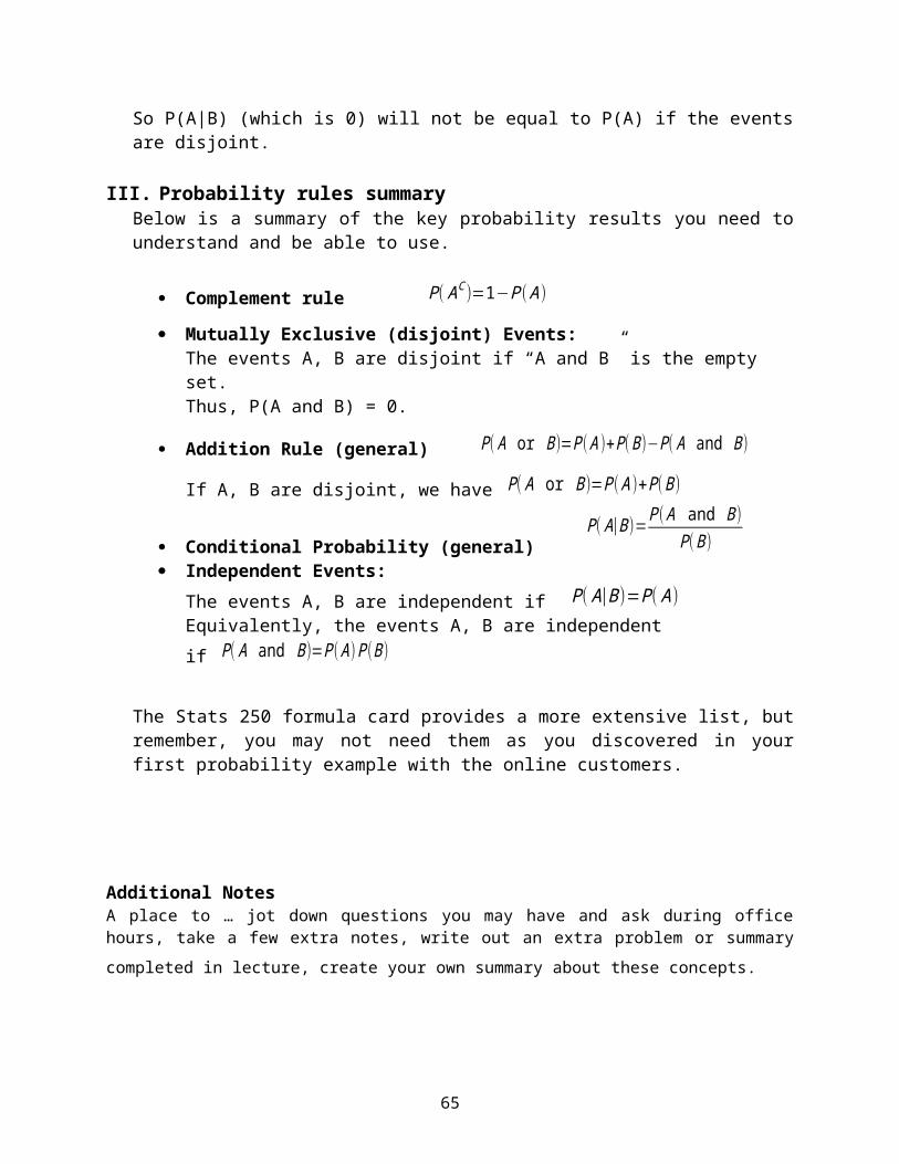
How to Solve General Normal Curve ProblemsOne way to find areas and thus probabilities for any general N ( μ ,σ ) distribution involves the idea of standardization.

If the variable X has the N ( μ ,σ ) distribution,

then the standardized variable Z= X−μ

σ will have the N (0,1 ) distribution.We will see how this standardization idea works through our next example.

Try It! Scholastic ScoresA proposal before the Board of Education has specified certain designations for elementary schools depending on how their students do on the Evaluation of Scholastic Scoring. This test is given to all students in all public schools in grades 2 through 4. Schools that score in the top 20% are labeled excellent. Schools in the bottom 25% are labeled "in danger" and schools in the bottom 5% are designated as failing. Previous data suggests that scores on this test are approximately normal with a mean of 75 and a standard deviation of 5.

a. What is the probability that a randomly selected school will score below 70?

66

b. What is the score cut-off required for schools to be labeled excellent? Show all work.

Notes:1. The normal distribution is a density for continuous random variables.2. The normal distribution is not the only continuous distribution (recall you worked with a

family of uniform continuous distributions a few pages back).3. Computers and calculators often have the ability to find areas or percentiles for many

density curves built right in to a function. You might be introduced to some of these in your lab sessions and are welcome to use them. But drawing a picture of what you are trying to find will be beneficial and serve as one way to show your work.

Approximating Binomial Distribution Probabilities

Recall Our Left-Handed ProblemIn an earlier problem it was stated that about 10% of Americans are left-handed. Let X = the number of left-handed Americans in a random sample of 120 Americans (part c had us think about a sample size being 120 instead of 12).

Then X has an exact Binomial distribution with n = 120 and p = 0.10. The mean or expected number of left-handed Americans in the sample is = np = 120(0.10) = 12. The standard

deviation of X is = √np(1−p )=√120(0 .10)(0 . 90 )= 3.29.

Suppose we want to find the probability that a random sample of 120 will contain 20 or fewer left-handed Americans. Using the exact binomial distribution we would start with:

P(X≤20)=P(X=0)+P(X=1)+⋯+P(X=19)+P( X=20 )

This would not be too much fun to compute by hand since each of the probabilities for X = 0 up

to X = 20 would be found using the binomial probability formula: P(X=k )=(nk ) pk (1−p)n−k

.But there is an easier way that will give us approximately the probability of having 20 or fewer. The easier way involves using a normal distribution. The normal distribution can be used to

67

approximate probabilities for other types of random variables, one being binomial random variables when the sample size n is large.

Normal Approximation to the Binomial DistributionIf X is a binomial random variable based on n trials with success probability p, and n is large, then the random variable X is also approximately …

Conditions: The approximation works well when both np and n(1 – p) are at least 10.

68

Try It! Returning to our Left-Handed ProblemAbout 10% of Americans are left-handed. Let X = the number of left-handed Americans in a random sample of 120 Americans. Then X has an exact Binomial distribution with n = 120 and p = 0.10. The mean number of left-handed Americans in the sample = np = 120(0.10) = 12.

And the standard deviation of X = = √np(1−p )=√120(0 . 10)(0 . 90 )= 3.29.

a. We want to find the probability that a random sample of 120 will contain 20 or fewer left-handed Americans. Since np = 120(0.10) = 12 and n(1 – p) = 120(0.90) = 108 are both at least 10, we can use the normal approximation for the distribution of X.

X has approximately a Normal distribution: N( _____, ______ )P(X≤20)=

b. How likely is it that more than 20% of the sample will be left-handed Americans?

Sums, Differences, and Combinations of Random VariablesThere are many instances where we want information about combinations of random variables. One type of combination of variables is a linear combination. Two primary linear combinations that arise are sums and differences.

Sum = X + Y Difference = X – YThe next two summary boxes present the rules for finding the mean and the variance (and thus standard deviation) of a sum and of a difference. We will see the results for a difference when we study learning about the difference between two proportions and about the difference between two means.Rules for Means:

Mean(X + Y) = Mean(X) + Mean(Y)Mean(X – Y) = Mean(X) – Mean(Y)

Rules for Variances (if X and Y are independent):Variance(X + Y) = Variance(X) + Variance(Y)Variance(X – Y) = Variance(X) + Variance(Y)

Think about it: why is the variance of a difference found by taking the sum of the variances?

69

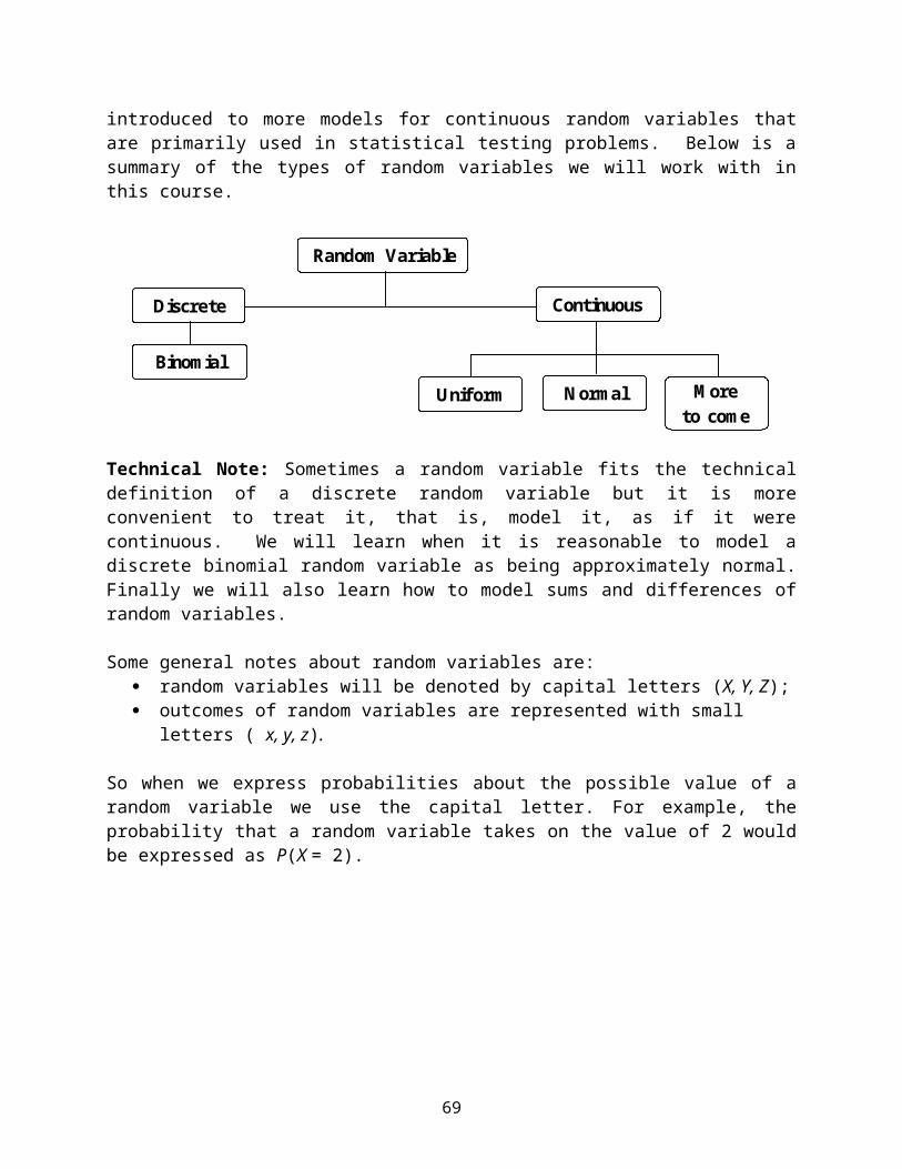
Additional NotesA place to … jot down questions you may have and ask during office hours, take a few extra notes, write out an extra problem or summary completed in lecture, create your own summary about these

concepts.

70

Stat 250 Gunderson Lecture Notes5: Learning about a Population Proportion

Part 1: Distribution for a Sample Proportion

To be a statistician is great!! You never have to be "absolutely sure" of something. Being "reasonably certain" is enough!

-- Pavel E. Guarisma, North Carolina State University

Recall: Parameters, Statistics, and Statistical Inference

Some distinctions to keep in mind: Population versus Sample Parameter versus Statistic

Population proportion p versus sample proportion pPopulation mean μ versus sample mean X

Since we hardly ever know the true population parameter value, we take a sample and use the sample statistic to estimate the parameter. When we do this, the sample statistic may not be equal to the population parameter, in fact, it could change every time we take a new sample. Will the observed sample statistic value be a reasonable estimate? If our sample is a RANDOM SAMPLE, then we will be able to say something about the accuracy of the estimation process.

Statistical Inference: the use of sample data to make judgments or decisions about populations.

The two most common statistical inference procedures are confidence interval estimation and hypothesis testing.

Confidence Interval Estimation: A confidence interval is a range of values that the researcher is fairly confident will cover the true, unknown value of the population parameter. In other words, we use a confidence interval to estimate the value of a population parameter. We have already encountered the idea of a margin of error and using it to form a confidence interval for a population proportion.

Hypothesis Testing: Hypothesis testing uses sample data to attempt to reject a hypothesis about the population. Usually researchers want to reject the notion that chance alone can explain the sample results. Hypothesis testing is applied to population parameters by specifying a null value for the parameter—a value that would indicate that nothing of interest is happening. Hypothesis testing proceeds by obtaining a sample, computing a sample statistic, and assessing how unlikely the sample statistic would be if the null parameter value were correct. In most cases, the researchers are trying to show that the null value is not correct. Achieving statistical significance is equivalent to rejecting the idea that the observed results are plausible if the null value is correct.

71

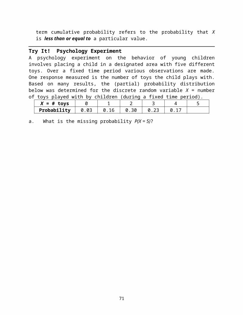
72

An Overview of Sampling DistributionsThe value of a statistic from a random sample will vary from sample to sample. So a statistic is a random variable and it will have a probability distribution. This probability distribution is called the sampling distribution of the statistic.

Definition: The distribution of all possible values of a statistic for repeated samples of the same size from a population is called the sampling distribution of the statistic.

We will study the sampling distribution of various statistics, many of which will have approximately normal distributions. The general structure of the sampling distribution is the same for each of the five scenarios. The sampling distribution results, along with the ideas of probability and random sample, play a vital role in the inference methods that we continue studying throughout the remainder of the course.

Sampling Distributions for One Sample ProportionMany responses of interest produce counts rather than measurements -- sex (male, female), political preference (republican, democrat), approve of new proposal (yes, no). We want to learn about a population proportion and we will do so using the information provided from a sample from the population.

Example: Do you work more than 40 hours per week?A poll was conducted by The Heldrich Center for Workforce Development (at Rutgers University). A probability sample of 1000 workers resulted in 460 (for 46%) stating they work more than 40 hours per week.

Population =

Parameter =

Sample =

Statistic =

Can anyone say how close this observed sample proportion p is to the true population proportion p ?

If we were to take another random sample of the same size n=1000 , would we get the same value for the sample proportion p ?

So what are the possible values for the sample proportion p if we took many random samples of the same size from this population? What would the distribution of the possible p values look like? What is the sampling distribution of p ?

73

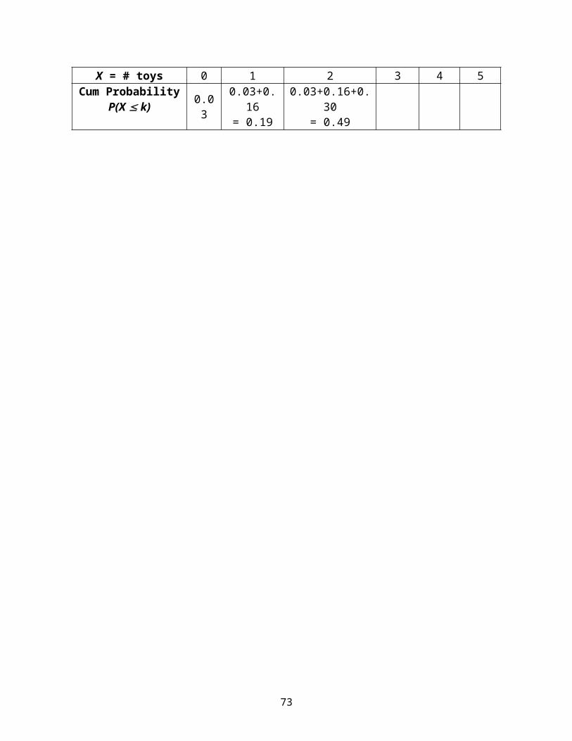
Aside: Can you Visualize It?Consider taking your one random sample of size n and computing your one p value. (As in the

previous example, our one p = 460/1000 = 0.46.) Suppose we did take another random sample of the same size, we would get another value of p , say ___________. Now repeat that process over and over; taking one random sample after another; resulting in one p value after another.

Example picture showing the possible values when n = _______

0 0.1 0.2 0.3 0.4 0.5 0.6 0.7 0.8 0.9 1 p values

Observations:

How would things change if the sample size n were even larger, say n = _____? Suppose our first sample proportion turned out to be p = _________ . Now imagine again repeating that process over and over; taking one random sample after another; resulting in many p possible

values.

Example picture showing the possible values when n = _______

0 0.1 0.2 0.3 0.4 0.5 0.6 0.7 0.8 0.9 1 p values

Observations:

74

75

Let’s take a closer look at the sample proportion p . The sample proportion is found by taking the number of “successes” in the sample and dividing by the sample size. So the count variable

X of the number of successes is directly related to the proportion of successes as p=Xn .

Earlier we studied the distribution of our first statistic, the count statistic X (the number of successes in n independent trials when the probability of a success was p). We learned about its exact distribution called the Binomial Distribution. We also learned when the sample size n was large, the distribution of X could be approximated with a normal distribution.

Normal Approximation to the Binomial Distribution

If X is a binomial random variable based on n trials with success probability p, and n is large,

then the random variable X is also approximately N (np ,√np(1−p )) .

Conditions: The approximation works well when both np and n(1 – p) are at least 10.

So any probability question about a sample proportion could be converted to a probability question about a sample count, and vice-versa. If n is small, we would need to convert the question to a count and use the binomial

distribution to work it out.

If n is large, we could convert the question to a count and use the normal approximation for a count, OR use a related normal approximation for a sample proportion (for large n).

The Stat 250 formula card summarizes this related normal approximation as follows:

Let’s put this result to work in our next Try It! Problem.

76

Try It! Do Americans really vote when they say they do?To answer this question, a telephone poll was taken two days an election. From the 800 adults polled, 56% reported that they had voted. However, it was later reported in the press that, in fact, only 39% of American adults had voted. Suppose the 39% rate reported by the press is the correct population proportion. Also assume the responses of the 800 adults polled can be viewed as a random sample.

a. Sketch the sampling distribution of p for a random sample of size n = 800 adults.

b. What is the approximate probability that a sample proportion who voted would be 56% or larger for a random sample of 800 adults?

c. Does it seem that the poll result of 56% simply reflects a sample that, by chance, voted with greater frequency than the general population?

More on the Standard Deviation of p

The standard deviation of p is given by: s.d.( p ) = √ p(1−p)n

This quantity would give us an idea about how far apart a sample proportion p and the true population proportion p are likely to be.

We can interpret this standard deviation as approximately the average distance of the

possible p values (for repeated samples of the same size n) from the true population proportion p.

77

In practice when we take a random sample from a large population, we only know the sample proportion. We generally would not know the true population proportion p. So we could not

compute the standard deviation of p . However we can use the sample proportion in the formula to have an estimate of the standard

deviation, which is called the standard error of p .

The standard error of p is given by: s.e.( p ) = √ p(1− p)n

This quantity is an estimate of the standard deviation of p .

So we can interpret this standard error as estimating, approximately, the average distance of

the possible p values (for repeated samples of the same size n) from the true population proportion p.

Moreover, we can use this standard error to create a range of values that we are very confident

will contain the true proportion p, namely, p (a few)s.e.( p ).

This is the basis for confidence interval for the true proportion p, discussed next

Try It! Love at first sight?In a random sample of n = 500 adults, 300 stated they believe in love at first sight. a. Estimate the population proportion of adults that believe in love at first sight.

b. Find the corresponding standard error of for the estimate in part a and use this standard error to provide an interval estimate for the population proportion p, with 95% confidence.

78

Stat 250 Gunderson Lecture Notes5: Learning about a Population Proportion

Part 2: Estimating Proportions with Confidence

Big Idea of Confidence Intervals: Use sample data to estimate a population parameter.

Recall some of the language and notation associated with the estimation process.

Population and Population Parameter Sample and Sample Statistic (sample estimate or point estimate)

The sample estimate provides our best guess as to what is the value of the population parameter, but it is not 100% accurate.

The value of the sample estimate will vary from one sample to the next. The values often vary around the population parameter and the standard deviation give an idea about how far the sample estimates tend to be from the true population proportion on average.

The standard error of the sample estimate provides an idea of how far away it would tend to vary from the parameter value (on average).

The general format for a confidence interval estimate is given by:Sample estimate ± (a few) standard errors

The “few” or number of standard errors we go out each way from the sample estimate will depend on how confident we want to be.

The “how confident” we want to be is referred to as the confidence level. This level reflects how confident we are in the procedure. Most of the intervals that are made will contain the truth about the population, but occasionally an interval will be produced that does not contain the true parameter value. Each interval either contains the population parameter or it doesn’t. The confidence level is the percentage of the time we expect the procedure to produce an interval that does contain the population parameter.

Confidence Interval for a Population Proportion pGoal: we want to learn about a population proportion p . How? We take a random sample

from the population and estimate p with the resulting sample proportion p . Let’s first recall how those many possible values for the sample proportion would vary, that is, the sampling

distribution of the statistic p .

79

Sampling Distribution of p : If the sample size n is large and np≥10 and n(1−p )≥10 ,

then p is approximately N ( p ,√ p(1−p)

n ).

Density N( , )

1. Consider the following interval or range of values and show it on the picture.

nppp

nppp

nppp 12,1212

2. What is the probability that a (yet to be computed) sample proportion p will be in this interval (within 2 standard deviations from the true proportion p)?

3. Take a possible sample proportion p and consider the interval

nppp

nppp

nppp 12ˆ,12ˆ12ˆ

Show this range on the normal distribution picture above.

4. Did your first interval around your first p contain the true proportion p? Was it a ‘good’ interval? __________

5. Repeat steps 3 and 4 for other possible values of p .

80

81

Big Idea: Consider all possible random samples of the same large size n. Each possible random sample provides a possible sample proportion value.

If we made a histogram of all of these possible p values it would look like the normal distribution on the previous page.

About 95% of the possible sample proportion p values will be in the interval n

ppp

12; and for each one of these sample proportion p values, the interval

n

ppp

12 will contain the population proportion p.

Thus about 95% of the intervals n

ppp

12ˆ will contain the population proportion p.

Thus, an initial 95% confidence interval for the true proportion p is given by: n

ppp 12ˆ

The Dilemma: When we take our one random sample, we can compute the sample

proportion p , but we can’t construct the interval

n

ppp 12ˆ

because we don’t know the value of p.

The Solution: Replace the value of p in the standard deviation with the estimate p ,

that is use

n

pp ˆ1ˆ

called ____________________.

An approximate 95% confidence interval (CI) for the population proportion p is:

p±2√ p(1− p )

n

Note: The part of the interval 2√ p(1− p )

n is called the 95% margin of error.

Note: The approximate is due to the multiplier of ‘2’ being used.

82

We will learn about other multipliers, including the exact 95% multiplier value later.

83

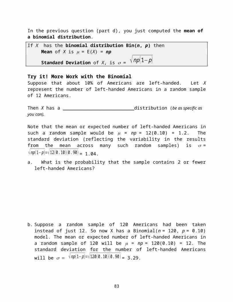
Try It! Getting Along with ParentsIn a Gallup Youth Survey n = 501 randomly selected American teenagers were asked about how well they get along with their parents. One survey result was that 54% of the sample said they get along “VERY WELL” with their parents.

a. The sample proportion was found to be 0.54. Give the standard error for the sample proportion and use it to complete the sentence that interprets the standard error in terms of an average distance.

We would estimate the average distance between the possible ______ values

(from repeated samples) and _____________________ to be about 0.022.

b. Compute a 95% confidence interval for the population proportion of teenagers that get along very well with their parents.

c. Fill in the blanks for the typical interpretation of the confidence interval in part b:

“Based on this sample, with 95% confidence, we would estimate that

somewhere between ________ and _______ of all American teenagers think they get

along very well with their parents.”

d. Can we say the probability that the above (already observed) interval (___________ , ___________) contains the population proportion p is 0.95?

That is, can we say ?95.0________)(_______ pP

e. Can we say that 95% of the time the population proportion p will be in the interval computed in part b?

84

Just what does the 95% confidence level mean? InterpretationThe phrase confidence level is used to describe the likeliness or chance that a yet-to-be constructed interval will actually contain the true population value. However, we have to be careful about how to interpret this level of confidence if we have already completed our interval.

The population proportion p is not a random quantity, it does not vary - once we have “looked” (computed) the actual interval, we cannot talk about probability or chance for this particular interval anymore. The 95% confidence level applies to the procedure, not to an individual interval; it applies “before you look” and not “after you look” at your data and compute your interval.

Try It! Getting Along with ParentsIn the previous Try It! you computed a 95% confidence interval for the population proportion of teenagers that get along very well with their parents in part (b). This was based on a random sample of n = 501 American teenagers. You interpreted the interval in part (c). Write a sentence or two that interprets the confidence level.

The interval we found was computed with a method which if repeated over and over ...

Try It! Completing a Graduate DegreeA researcher has taken a random sample of n = 100 recent college graduates and recorded whether or not the student completed their degree in 5 years or less. Based on these data, a 95% confidence interval for the population proportion of all college students that complete their degree in 5 years or less is computed to be (0.62, 0.80). a. How many of the 100 sampled college graduates completed their degree in 5 years or less?

b. Which of the following statements gives a valid interpretation of this 95% confidence level? Circle all that are valid.

i. There is about a 95% chance that the population proportion of students who have completed their degree in 5 years or less is between 0.62 and 0.80.

ii. If the sampling procedure were repeated many times, then approximately 95% of the resulting confidence intervals would contain the population proportion of students who have completed their degree in 5 years or less.

iii. The probability that the population proportion p falls between 0.62 and 0.80 is 0.95 for repeated samples of the same size from the same population.

85

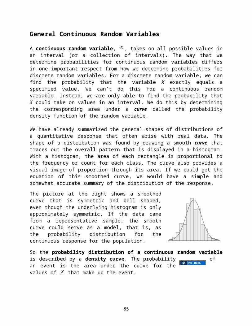
What about that Multiplier of 2?The exact multiplier of the standard error for a 95% confidence level would be 1.96, which was rounded to the value of 2. Where does the 1.96 come from? Use the standard normal distribution, the N(0, 1) distribution at the right and Table A.1.

Researchers may not always want to use a 95% confidence level. Other common levels are 90%, 98% and 99%.

Using the same idea for confirming the value of 1.96, find the correct multiplier if the confidence level were 90%.

The generic expression for this multiplier when you are working with a standard normal distribution is given by z*.

Here are a few other multipliers for a population proportion confidence interval. Confidence Level 90% 95% 98% 99%

Multiplier z* 1.645 1.96 (or about 2) 2.326 2.576 Now, the easiest way to find multipliers is to actually look ahead a bit and make use of Table A.2. Look at the df row marked Infinite degrees of freedom and you will find the z* values for many common confidence levels. Check it out!

…

From Utts, Jessica M. and Robert F. Heckard. Mind on Statistics, Fourth Edition. 2012. Used with permission.

When the confidence level increases, the value of the multiplier increases. So the width of the confidence interval also increases. In order to be more confident in the procedure (have a procedure with a higher probability of producing an interval that will contain the population

86

value, we have to sacrifice and have a wider interval. The formula for a confidence interval for a population proportion p is summarized next.

Confidence Interval for a Population Proportion p: )ˆ(s.e.ˆ * pzp

where p is the sample proportion and *z is the appropriate multiplier

and s.e.( p ) =

n

pp ˆ1ˆ

is the standard error of the sample proportion.Conditions:1. The sample is a randomly selected sample from the population. However, available data

can be used to make inferences about a much larger group if the data can be considered to be representative with regard to the question(s) of interest.

2. The sample size n is large enough so that the normal curve approximation holds 10np and 10)1( pn

Try It! A 90% CI for p A random sample of n = 501 American teenagers resulted in 54% stating they get along very well with their parents. The standard error for this estimate was found to be 2.2%. The 95% confidence interval for the population proportion of teenagers that get along very well with their parents went from 49.6% to 58.4%. The corresponding 90% confidence interval would go from 50.4% to 57.6%, which is indeed narrower (but still centered around the estimate of 54%).

The Conservative Approach From the general form of the confidence interval, the margin of error is given as:

Margin of error = z* s.e.( p ) = z*

n

pp ˆ1ˆ

For any fixed sample size n, this margin of error will be the largest when p = ½ = 0.5. Think

about the function p(1− p ) . So using ½ for p in the above margin of error expression we have:

z¿√ p(1− p)n =z¿√ 1

2(1−1

2 )

n = z¿

2√nBy using this margin of error for computing a confidence interval, we are being conservative. The resulting interval may be a little wider than needed, but it will not err on being too narrow. This leads to a corresponding conservative confidence interval for a population proportion.

Conservative Confidence Interval for a Population Proportion p

nzp

2*ˆ

where p is the sample proportion and *z is the appropriate multiplier.

87

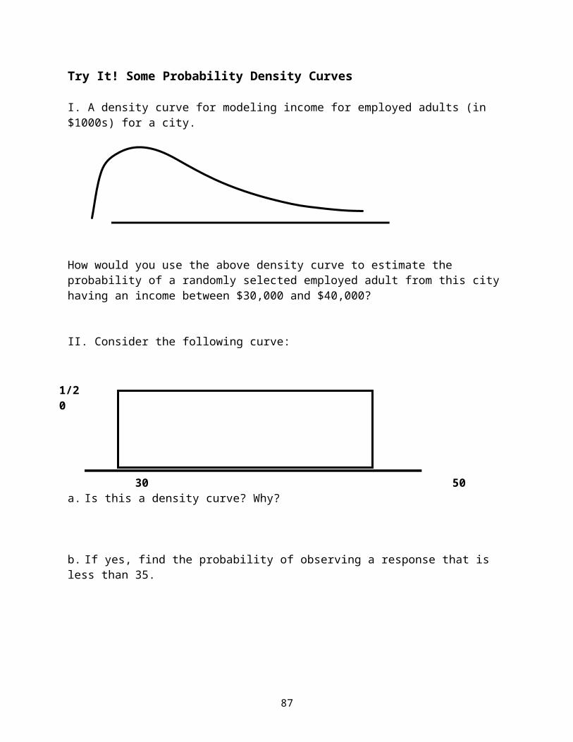
Earlier we saw the margin of error for a proportion was given as 1√n . This is actually a 95%

conservative margin of error. What happens to the conservative margin of error in the box above when you use *z = 2 for 95% confidence? Choosing a Sample Size for a SurveyThe choice of a sample size is important in planning a survey. Often a sample size is selected (using the conservative approach) that such that it will produce a desired margin of error for a given level of confidence. Let’s take a look at the conservative margin of error more closely.

(Conservative) Margin of Error = m =

z¿

2√n

Solving this expression for the sample size n we have: n=( z¿

2m )2

If this does is not a whole number, we would round up to the next largest integer.

Try It! Coke versus PepsiA poll was conducted in Canada to estimate p, the proportion of Canadian college students who prefer Coke over Pepsi. Based on the sampled results, a 95% conservative confidence interval for p was found to be (0.62, 0.70).a. What is the margin of error for this interval?

b. What sample size would be necessary in order to get a conservative 95% confidence interval for p with a margin of error of 0.03 (that is, an interval with a width of 0.06)?

c. Suppose that the same poll was repeated in the United States (whose population is 10 times larger than Canada), but four times the number of people were interviewed. The resulting 95% conservative confidence interval for p will be:

twice as wide as the Canadian interval 1/2 as wide as the Canadian interval 1/4 as wide as the Canadian interval 1/10 as wide as the Canadian interval the same width as the Canadian interval

Using Confidence Intervals to Guide DecisionsThink about it: A value that is not in a confidence interval can be rejected as a likely value of the population proportion. A value that is in a confidence interval is an “acceptable” possibility for the value of a population proportion.

88

Try It! Coke versus PepsiRecall the poll conducted in Canada to estimate p, the proportion of Canadian college students who prefer Coke over Pepsi. Based on the sampled results, a 95% conservative confidence interval for p was found to be (0.62, 0.70). Do you think it is reasonable to conclude that a majority of Canadian college students prefer Coke over Pepsi? Explain.

Additional NotesA place to … jot down questions you may have and ask during office hours, take a few extra notes, write out an extra problem or summary completed in lecture,

create your own summary about these concepts.

89

90

Stat 250 Gunderson Lecture Notes5: Learning about a Population Proportion

Part 3: Testing about a Population ProportionWe make decisions in the dark of data. -- Stu Hunter

Overview of Testing TheoriesWe have examined statistical methods for estimating the population proportion based on the sample proportion using a confidence interval estimate. Now we turn to methods for testing theories about the population proportion. The hypothesis testing method uses data from a sample to judge whether or not a statement about a population is reasonable or not. We want to test theories about a population proportion and we will do so using the information provided from a sample from the population.

Basic Steps in Any Hypothesis TestStep 1: Determine the null and alternative hypotheses.

Step 2: Verify necessary data conditions, and if met, summarize the data into an appropriate test statistic.

Step 3: Assuming the null hypothesis is true, find the p-value.

Step 4: Decide whether or not the result is statistically significant based on the p-value.

Step 5: Report the conclusion in the context of the situation.

Formulating Hypothesis StatementsMany questions in research can be expressed as which of two statements might be correct for a population. These two statements are called the null and the alternative hypotheses.

The null hypothesis is often denoted by H0, and is a statement that there is no effect, no difference, that nothing has change or nothing is happening. The null hypothesis is usually referred to as the status quo.

The alternative hypothesis is often denoted by Ha, and is a statement that there is a relationship, there is a difference, that something has changed or something is happening.

Usually the researcher hopes the data will be strong enough to reject the null hypothesis and support the new theory in the alternative hypothesis.

It is important to remember that the null and alternative hypotheses are statements about a population parameter (not about the results in the sample). Finally, there will often be a “direction of extreme” that is indicated by the alternative hypothesis. To see these ideas, let's try writing out some hypotheses to be put to the test.

91

Try It! Stating the Hypotheses and defining the parameter of interest

1. About 10% of the human population is left-handed. Suppose that a researcher speculates that artists are more likely to be left-handed than are other people in the general population.

H0:let ________ =_________________________________

Ha: parameter = written description

Direction:

2. Suppose that a pharmaceutical company wants to be able to claim that for its newest medication the proportion of patients who experience side effects is less than 20%.

H0:let ________ =_________________________________

Ha: parameter = written description

Direction:

3. The US Census reports that 48% of households have no children. A random sample of 500 households will be taken to assess if the population proportion has changed from the Census value of 0.48.

H0:let ________ =_________________________________

Ha: parameter = written description

Direction:

Notes:1. When the alternative hypothesis specifies a single direction, the test is called a one-sided or

one-tailed hypothesis test. In practice, most hypothesis tests are one-sided tests because investigators usually have a particular direction in mind when they consider a question.

2. When the alternative hypothesis includes values in both direction from a specific standard, the test is called a two-sided or two-tailed hypothesis test.

3. A generic null hypothesis could be expressed as H0: population parameter = null value, where the null value is the specific number the parameter equals if the null hypothesis is true. In all of the examples above, the population parameter is p, the population proportion. Example 1 above has the null value of 10% or 0.10.

92

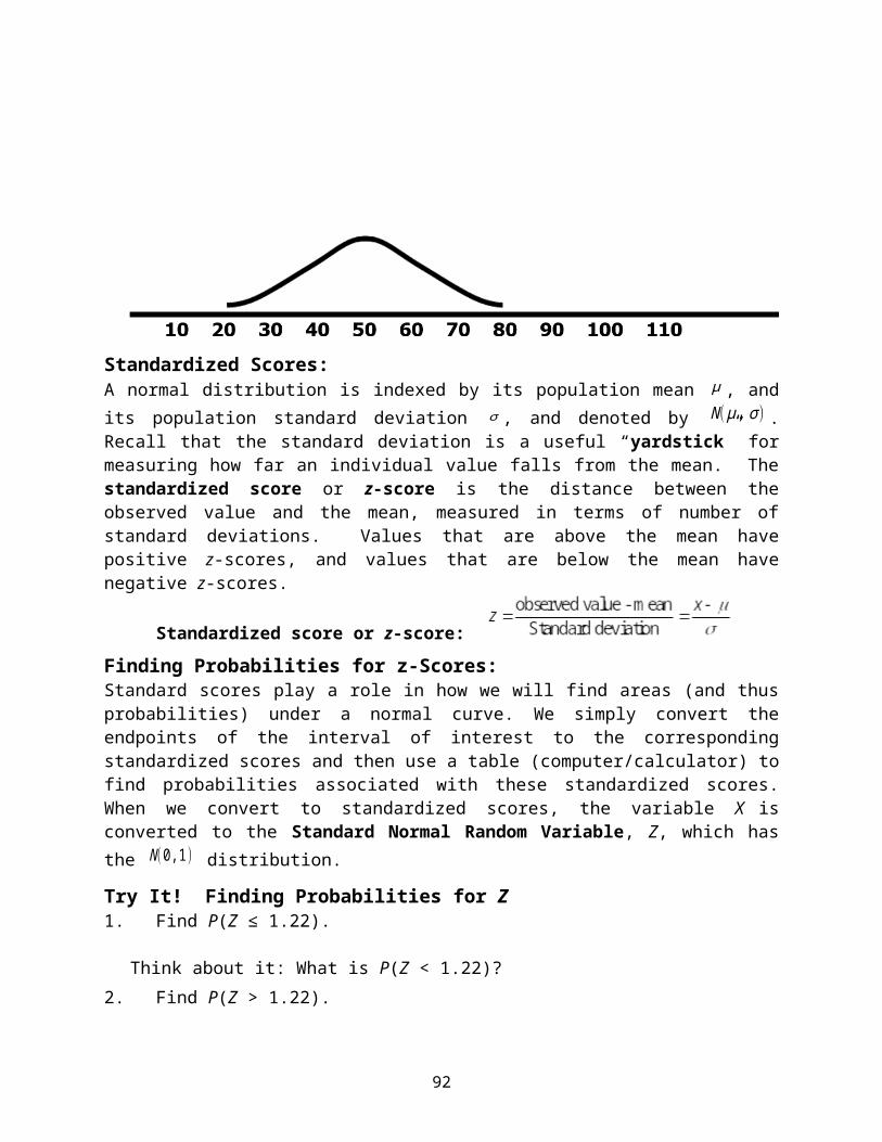
The Logic of Hypothesis Testing: What if the Null is True?Think about a jury trial …

H0: The defendant is _______________ Ha: The defendant is _______________

We assume that the null hypothesis is true until the sample data conclusively demonstrate otherwise. We assess whether or not the observed data are consistent with the null hypothesis (allowing reasonable variability). If the data are “unlikely” when the null hypothesis is true, we would reject the null hypothesis and support the alternative theory.

The Big Question we ask: If the null hypothesis is true about the population, what is the probability of observing sample data like that observed (or more extreme)?

Reaching Conclusions about the Two HypothesesWe will be deciding between the two hypotheses using data. The data is assumed to be a random sample from the population under study.

The data will be summarized via a ________________________________. In many cases the test statistic is a standardized statistic that measures the distance between the sample statistic and the null value in standard error units.

Test Statistic = Sample Statistic – Null Value (Null) Standard Error

In fact, our first test statistic will be a z-score and we are already familiar with what makes a z-value unusual or large.

With the test statistic computed, we quantify the compatibility of the result with the null hypothesis with a probability value called the p-value.

The p-value is computed by assuming the null hypothesis is true and then determining the probability of a result as extreme (or more extreme) as the observed test statistic in the direction of the alternative hypothesis.

Notes: (1) The p-value is a probability, so it must be between 0 and 1. It is really a conditional

probability – the probability of seeing a test statistic as extreme or more extreme than observed given (or conditional on) the null hypothesis is true.

(2) The p-value is not the probability that the null hypothesis is true.

The ____________________ the p-value, the stronger the evidence is AGAINST H0 (and in favor of Ha).

Common Convention: Reject H0 if the p-value is ___________________________.

This borderline value is called the ____________________ and denoted by _____.

When the p-value is we say the result is ______________________________.

Common levels of significance are: _________________________________

93

Two Possible Results: The p -value is so we reject H 0

and say the results are statistically significant at the level We would then write a real-world conclusion to explain what ‘rejecting H0’ translates to in the context of the problem at hand.

The p -value is > , so we fail to reject H 0 and say the results are not statistically significant at the level . We would then write a real-world conclusion to explain what ‘failing to reject H0’ translates to in the context of the problem at hand.

Be careful: we say “fail to reject H0” and not “accept H0” because the data do not prove the null hypothesis is true, rather the data were not convincing enough to support the alternative hypothesis.

Testing Hypotheses About a Population ProportionIn the context of testing about the value of a population proportion p, the possible hypotheses statements are:

1. H0: _________________ versus Ha: ___________________

2. H0: _________________ versus Ha: ___________________

3. H0: _________________ versus Ha: ___________________

Where does p0 come from? Sometimes the null hypothesis is written as H0:p = p0 as we compute the p-value assuming the null hypothesis is true, that is, we take the population proportion to be the null value p0.

The sample data will provide us with an estimate of the population proportion p, namely the sample proportion p . For a large sample size, the distribution for the sample proportion will be:

If we have a normal distribution for a variable, then we can standardize that variable to compute probabilities, as long as you have the mean and standard deviation for that statistic. In testing, we assume that the null hypothesis is true, that the population proportion p = p0. So the standardized z-statistic for a sample proportion in testing is:

z =

If the null hypothesis is true, this z-test statistic will have approximately a _________________.

94

The standard normal distribution will be used to compute the p-value for the test.

95

Try It! Left-handed ArtistsAbout 10% of the human population is left-handed. Suppose that a researcher speculates that artists are more likely to be left-handed than are other people in the general population. The researcher surveys a random sample of 150 artists and finds that 18 of them are left-handed. Perform the test using a 5% significance level.

Step 1: Determine the null and alternative hypotheses.

H0: ___________________ Ha: ____________________

where the parameter _____ represents _________________________

_________________________________________________________

Note: The direction of extreme is

Step 2: Verify necessary data conditions, and if met, summarize the data into an appropriate test statistic. The data are assumed to be a random sample. Check if np0 10 and n(1 – p0) 10.

Observed test statistic: npp

ppz

)1(

ˆ

00

0

Step 3: Assuming the null hypothesis is true, find the p-value.The p-value is the probability of getting a test statistic as extreme or more extreme than the observed test statistic value, assuming the null hypothesis is true. Since we have a one-sided test to the right, toward the larger values …

p-value = probability of getting a z test statistic as large or larger than observed, assuming the null hypothesis is true.

=

Step 4: Decide if the result is statistically significant based on the p-value.

Step 5: Report the conclusion in the context of the situation.

96

Aside: The researcher chooses the level of significance before the study is conducted. In our Left-Handed Artists example we had H0: p = 0.10 versus Ha: p > 0.10. If only 12 LH artists in our sample,

we would have p = 0.08, we would certainly not reject H0

With our 18 LH artists in our sample, our p = 0.12, z=0.82, p-value=0.206 and our decision was to fail to reject H0

What if we had 20 LH artists in our sample, our p = 0.133, our z=1.36, p-value=0.0868 and our decision would be_____________

What if we had 22 LH artists in our sample, our p = 0.147, our z=1.91, p-value=0.0284 and our decision would be_____________

What if we had 24 LH artists in our sample, our p = 0.16, our z=2.45, p-value=0.007, and our decision would be _____________

Selecting the level of significance is like drawing a line in the sand – separating when you will reject H0 and when there the evidence would be strong enough to reject H0.

This first test was a one-sided test to the right. How is the p-value found for the other directions of extreme? The table below provides a nice summary.

From Utts, Jessica M. and Robert F. Heckard. Mind on Statistics, Fourth Edition. 2012. Used with permission.

97

Try It! Households without ChildrenThe US Census reports that 48% of households have no children. A random sample of 500 households was taken to assess if the population proportion has changed from the Census value of 0.48. Of the 500 households, 220 had no children. Use a 10% significance level.

Step 1: Determine the null and alternative hypotheses.

H0: p = 0.48 Ha: p ≠ 0.48

where the parameter p represents the population proportion of all households today that have no children. Note: The direction of extreme is two-sided.

Step 2: Verify necessary data conditions, and if met, summarize the data into an appropriate test statistic. The data are assumed to be a random sample. Check if np0 10 and n(1 – p0) 10.

Observed test statistic: npp

ppz

)1(

ˆ

00

0

Step 3: Assuming the null hypothesis is true, find the p-value.

The p-value is the probability of getting a test statistic as extreme or more extreme than the observed test statistic value, assuming the null hypothesis is true. Since we have a two-sided test, both large and small values are “extreme”.Sketch the area that corresponds to the p-value:

Compute the p-value:

Step 4: Decide if the result is statistically significant based on the p-value.

Step 5: Report the conclusion in the context of the situation.

98

What if n is small?

Goal: we still want to learn about a population proportion p. We take a random sample of size n where n is small (i.e. np0 < 10 or n(1 – p0) < 10). If the sample size is small, we have to go back to the exact distribution for a count X, called the binomial distribution.

If X has the binomial distribution Bin(n, p), thenknk pp

kn

kXP

)1()(

for nk ,...,2,1,0 where (nk )= n!

k !(n−k )!

and the mean of npX and the standard deviation of )1( pnpX

We will use the binomial probability formula for computing the exact p-value.

Testing Hypotheses about a Population Proportion p when n is smallWith a small sample size, we will do a Binomial test.

Small-Sample Binomial Test for the population proportion p To test the hypothesis H0: p = p0 we compute the count test statistic

X = the number of successes in the sample of size n which has the Bin(n, p0) distribution when H0 is true.

This Bin(n, p0), distribution is used to compute the p-value for the test.

Try It! New TreatmentA group of 10 subjects with a disease are treated with a new treatment. Of the 10 subjects, 9 showed improvement. Test the claim that “a majority” of people using this treatment improved using a 5% significance level. Let p be the true population proportion of people who improve with this treatment.

State the hypotheses: H0: ___________________ Ha: _________________

The observed test statistic value is just ___________________

p-value =

At the 5% significance level, we would and conclude:

99

100

Let’s revisit the flow chart for working on problems that deal with a population proportion.When the sample size is large we can use the large sample normal approximation for computing probabilities about a sample proportion, for testing hypotheses about a population proportion (based on the resulting sample proportion), and for computing a confidence interval estimate for the value of a population proportion (again using the sample proportion as the point estimate).

When the sample size is small we use the binomial distribution to compute probabilities about a sample proportion or to test hypotheses about a population proportion (based on the resulting sample count of successes). We did not discuss the small sample confidence interval for a population proportion using the binomial distribution.

Sample Size, Statistical Significance, and Practical ImportanceThe size of the sample affects our ability to make firm conclusions based on that sample. With a small sample, we may not be able to conclude anything. With large samples, we are more likely to find statistically significant results even though the actual size of the effect is very small and perhaps unimportant. The phrase statistically significant only means that the data are strong enough to reject the null hypothesis. The p-value tells us about the statistical significance of the effect, but it does not tell us about the size of the effect.

Consider testing H0: p = 0.5 versus Ha: p > 0.5 at = 0.05.Case 1: 52 successes in a sample of size n = 100 p = 0.52

Test Statistic: z = (0.52 - 0.50) / √ [0.5(1-0.5)/100] = 0.4 p-value = P(Z ≥ 0.4) = 0.34. So we would fail to reject H0. An increase of only 0.02 beyond 0.50 seems inconsequential (not significant).

Case 2: 520 successes in a sample of size n = 1000 p = 0.52 Test Statistic: z = (0.52 - 0.50) / √ [0.5(1-0.5)/1000] = 1.26 p-value = P(Z ≥ 1.26) = 0.104. So we would again fail to reject H0. Here an increase of 0.02 beyond 0.50 is approaching significance.

Case 3: 5200 successes in a sample of size n = 10,000 p = 0.52 Test Statistic: z = (0.52 - 0.50) / √ [0.5(1-0.5)/10,000] = 4.0 p-value = P(Z ≥ 4) = 0.00003. So we would certainly reject H0. Here an increase of 0.02 beyond 0.50 is very significant!

Convert to count Use X ~ N(np,np(1-p))

Use p-hat p-hat ~ N(p,p(1-p)/ n)

How to deal with questions about proportions

Proportions Response Variable is Categorical

with 2 outcomes: S, F

n is small Convert to count. Use X ~ Bin(n,p)

n is large np 10 and n(1-p) 10

or

101

Small samples make it very difficult to demonstrate much of anything. Huge sample sizes can make a practically unimportant difference statistically significant. Key: determine appropriate sample sizes so findings that are practically important become statistically significant.

What Can Go Wrong: Two Types of ErrorsWe have been discussing a statistical technique for making a decision between two competing theories about a population. We base the decision on the results of a random sample from that population. There is the possibility of making a mistake. In fact there are two types of error that we could make in hypothesis testing.

Type 1 error = rejecting H0 when H0 is true Type 2 error = failing to reject H0 when Ha is true

In statistics we have notation to represent the probabilities that a testing procedure will make these two types of errors.

P(Type 1 error) =P(Type 2 error) =

There is another probability that is of interest to researchers – if there really is something going on (if the alternative theory is really true), what is the probability that we will be able to detect it (be able to reject H0)? This probability is called the power of the test and is related to the probability of making a Type 2 error.

Power = P(rejecting H0 when Ha is true) = 1 – P(failing to reject H0 when Ha is true) = 1 – P(Type 2 error) = 1 – .

So we can think of power as the probability of advocating the “new theory” given the “new theory” is true. Researchers are generally interested in having a test with high power. One dilemma is that the best way to increase power is to increase sample size n (see comments below) and that can be expensive.

Comments:1. In practice we want to protect the status quo so we are most concerned with _____.2. Most tests we describe have the ...

3. Generally, for a fixed sample size n, ...

4. Ideally we want the probabilities of making a mistake to be small, we want the power of the test to be large. However, these probabilities are properties of the procedure (the proportion of times the mistake would occur if the procedure were repeated many times) and not applicable to the decision once it is made.

5. Some factors that influence the power of the test … Sample size: larger sample size leads to higher power. Significance level: larger leads to higher power.

102

Actual parameter value: a true value that falls further from the null value (in the direction of the alternative hypothesis) leads to higher power (however this is not something that the researcher can control or change).

103

Simple Example

H0: Basket has 9 Red and 1 WhiteHa: Basket has 4 Red and 6 White

Data: 1 ball selected at random from the basket.

What is the most reasonable Decision Rule?

Reject the null hypothesis if the ball is ___________________

With this rule, what are the chances of making a mistake?

P(Type 1 error) =

P(Type 2 error) =

What is the power of the test?

Suppose a ball is now selected from the basket and it is observed and found to be WHITE. What is the decision?

You just made a decision, could a mistake have been made? If so, which type?

What is the probability that this type of mistake was made?

Note: The Decision Rule stated in the simple example resembles the rejection region approach to hypothesis testing. We will focus primarily on the p-value approach that is used in reporting results in journals.

104

Additional NotesA place to … jot down questions you may have and ask during office hours, take a few extra notes, write out an extra problem or summary completed in lecture,

create your own summary about these concepts.

105

Stat 250 Gunderson Lecture Notes6: Learning about the Difference in Population Proportions

Part 1: Distribution for a Difference in Sample Proportions

The Independent Samples ScenarioTwo samples are said to be independent samples when the measurements in one sample are not related to the measurements in the other sample. Independent samples are generated in a variety of ways. Some common ways:

Random samples are taken separately from two populations and the same response variable is recorded for each individual.

One random sample is taken and a variable is recorded for each individual, but then units are categorized as belonging to one population or another, e.g. male/female.

Participants are randomly assigned to one of two treatment conditions, and the same response variable, such as weight loss, is recorded for each individual unit.

If the response variable is categorical, a researcher might compare two independent groups by looking at the difference between the two proportions.

There are usually two questions of interest about a difference in two population proportions. First, we want to estimate the value of the difference. Second, often we want to test the hypothesis that the difference is 0, which would indicate that the two proportions are equal. In either case, we will need to know about the sampling distribution for the difference in two sample proportions (from independent samples).

Sampling Distribution for the Difference in Two Sample Proportions

Example: Driving SafelyQuestion of interest: How much of a difference is there between men and women with regard to the proportion who have driven a car when they had too much alcohol to drive safely?

Study: Time magazine reported the results of a poll of adult Americans. One question asked was: “Have you ever driven a car when you probably had too much alcohol to drive safely?”

Let p1 be the population proportion of men who would respond yes.

Let p2 be the population proportion of women who would respond yes.

We want to learn about p1 and p2 and how they compare to each other. We could estimate the

difference p1 – p2 with the corresponding difference in the sample proportions 21 ˆˆ pp .

Will it be a good estimate? How close can we expect the difference in sample proportions to be to the true difference in population proportions (on average)?

106

Imagine repeating the study many times, each time taking two independent random samples of

sizes n1 and n2, and computing the value of 21 ˆˆ pp . What kind of values could you get for 21 ˆˆ pp ? What would the distribution of the possible 21 ˆˆ pp values look like? What can we

say about the distribution of the difference in two sample proportions?

Using results about how to work with differences of independent random variables and recalling the form of the sampling distribution for a sample proportion, the sampling

distribution of the difference in two sample proportions 21 ˆˆ pp can be determined.

First recall that when working with the difference in two independent random variables:

the mean of the difference is just the difference in the two means

the variance of the difference is the sum of the variances

Next, remember that the standard deviation of a sample proportion is √ p (1−p)n .

So what would the variance of a single sample proportion be?

So let’s apply these ideas to our newest parameter of interest, the difference in two sample

proportions 21 ˆˆ pp .

Sampling Distribution of the Difference in Two (Independent) Sample Proportions

If the two sample proportions are based on independent random samples from two

populations and if all of the quantities n1 p1 , n1 (1− p1 ), n2 p2 , and n2 (1− p2 ) are at least 10,

Then the distribution for the possible 21 ˆˆ pp will be (approximately) …

107

Since the population proportions of p1 and p2 are not known, we will use the data to compute the standard error of the difference in sample proportions.

Standard Error of the Difference in Sample Proportions

s .e .( p1− p2)=√ p1(1− p1)n1

+p2(1− p2 )

n2

The standard error of 21 ˆˆ pp estimates, roughly, the average distance of the possible

21 ˆˆ pp values from p1 – p2. The possible 21 ˆˆ pp values result from considering all possible independent random samples of the same sizes from the same two populations.

Moreover, we can use this standard error to produce a range of values that we can be quite confident will contain the difference in the population proportions p1 – p2:

21 ˆˆ pp (a few)s.e.( 21 ˆˆ pp ).

This is the basis for confidence interval for the difference in population proportions discussed next in Part 2.

If we are interested in testing hypotheses about the difference in the population rates, we will need to construct a null standard error of the difference in the sample proportions and use it to compute a standardized test statistic. That test statistic will have the following basic form:

Sample statistic – Null value. (Null) standard error

This is the basis for the hypothesis testing about the difference in population proportions covered in Part 3 of this section of notes.

108

Additional NotesA place to … jot down questions you may have and ask during office hours, take a few extra notes, write out an extra problem or summary completed in lecture, create your own summary about these

concepts.

109

Stat 250 Gunderson Lecture Notes6: Learning about the Difference in Population ProportionsPart 2: Confidence Interval for a Difference in Population Proportions

We have two populations from which independent samples are available, (or one population for which two groups formed using a categorical variable). The response variable is also categorical and we are interested in comparing the proportions for the two populations.

Let p1 be the population proportion for the first population. Let p2 be the population proportion for the second population.

Parameter: the difference in the population proportions p1 – p2.

Sample estimate: the difference in the sample proportions 21 ˆˆ pp .

Standard error: s .e .( p1− p2)=√ p1(1− p1)

n1+p2(1− p2 )

n2

So we have our estimate of the difference in the two population proportions, namely 21 ˆˆ pp , and we have its standard error. To make our confidence interval, we need to know the multiplier.

Sample Estimate Multiplier x Standard error

As in the case for estimating one population proportion, we assume the sample sizes are sufficiently large so the multiplier will be a z* value found from using the standard normal distribution.

Two Independent-Samples z Confidence Interval for p1 - p2

21*

21 ˆˆs.e.ˆˆ ppzpp

where s .e .( p1− p2)=√ p1(1−p1)

n1+p2(1− p2 )

n2

and z* is the appropriate multiplier from the N(0,1) distribution.

This interval requires that the sample proportions are based on independent random samples from the two populations.

110

Also, all of the quantities 11 pn , )ˆ1( 11 pn , 22 pn , and )ˆ1( 22 pn be preferably at least 10.

111

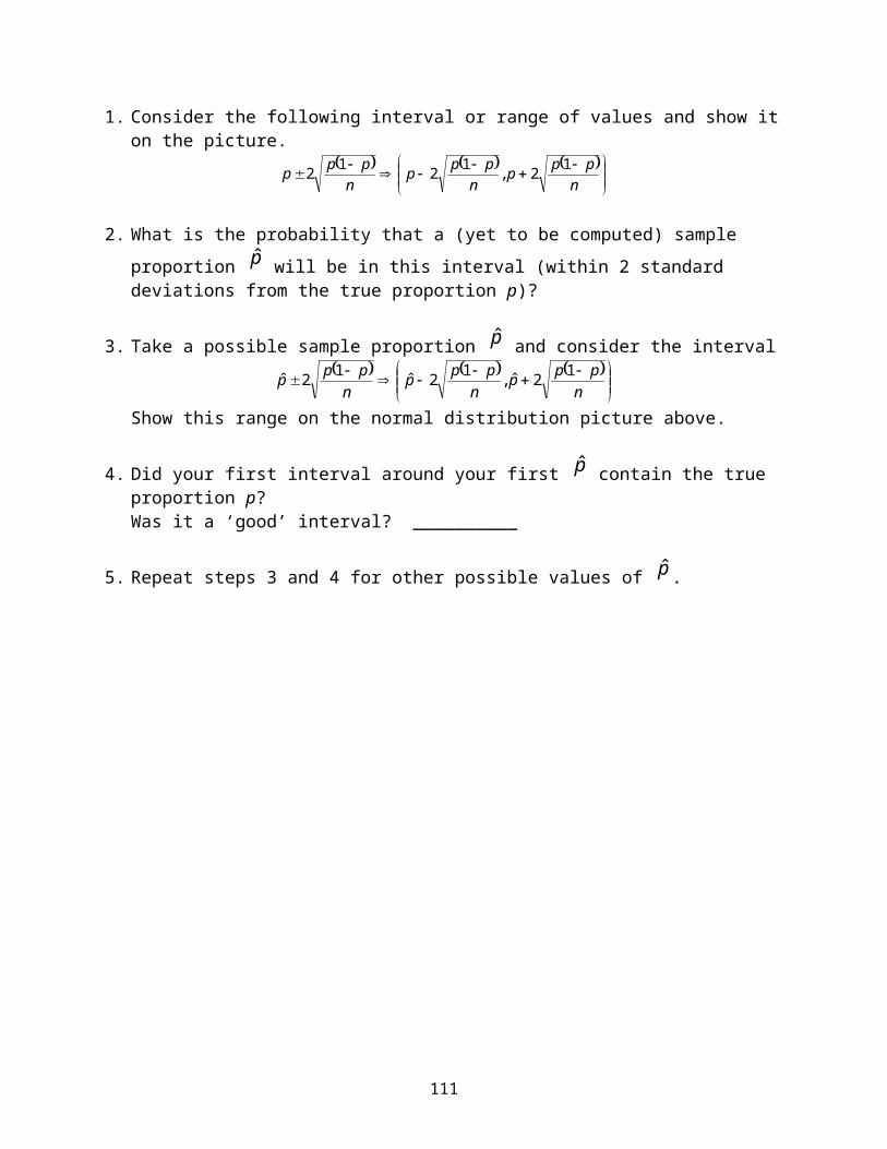
Try It! Do Older People Snore More than Younger?

Researchers at the National Sleep Foundation were interested in comparing the proportion of people who snore for two age populations (1 = older adults defined as over 50 years old and 2 = younger adults defined as between 18 and 30 years old). The following data was obtained from adults who participated in a sleep lab study.

“Snore?”Group Yes No Total 1 = older adults (over 50 years old) 168 312 480 2 = younger adults (between 18 and 30 years old) 45 135 180

Let p2 represent the population proportion of all younger adults who snore. Provide an estimate for this population proportion p2. Include the appropriate symbol.

We wish to provide a 90% confidence interval to estimate the difference in snoring rates for the two population proportions of adults. One of the conditions for that confidence interval to be valid involves having two independent random samples, which is reasonable from the design of the study. Validate the remaining assumption.

Provide the 90% confidence interval and give an interpretation of this interval in context.

Interpretation this interval. With 95% confidence we estimate the difference in snoring rates for the two population

of adults to be somewhere between ____________ and ____________.

What value do you notice is not in this interval? _________Does there appear to be a significant difference betweenthe population rates of snoring for older versus younger adults? Yes No

112

Stat 250 Gunderson Lecture Notes6: Learning about the Difference in Population Proportions

Part 3: Testing about a Difference in Population Proportions

Testing Hypotheses about the Difference in Two Population Proportions

We have two populations from which independent samples are available, (or one population for which two groups can be formed using a categorical variable). The response variable is also categorical and we are interested in comparing the proportions for the two populations.

Let p1 be the population proportion for the first population. Let p2 be the population proportion for the second population.

Parameter: the difference in the population proportions p1 – p2.

Sample estimate: the difference in the sample proportions 21 ˆˆ pp .

Standard error of 21 ˆˆ pp :

Recall that the multiplier in the confidence interval was a z* value. So we will be computing a Z test statistic for performing a significance test.

The standard error used in constructing the confidence interval for the difference between two population proportions is not the same as that used for the standardized z test statistic.

We will need to construct the null standard error, the standard error for the statistic when the null hypothesis is true. Let’s start with what the hypotheses will look like.

Possible null and alternative hypotheses.

1. H0: versus Ha:

2. H0: versus Ha:

3. H0: versus Ha:

113

Next we need to determine the test statistic and understand the conditions required for the test to be valid. The general form of the test statistic is:

Test statistic = Sample statistic – Null value Standard error

In the case of two population proportions, if the null hypothesis is true, we have p1 - p2 = 0 or that the two population proportions are the same, p1 = p2 = p. What is a reasonable way to estimate the common population proportion p?

The general standard error for 21 ˆˆ pp is given by:

s .e .( p1− p2)=√ p1(1− p1)n1

+p2(1− p2)

n2

but if the null hypothesis is true, then p is the best estimate for each population proportion and should be used in the standard error.

So, the null standard error for 21 ˆˆ pp is given by:

And the corresponding test statistic is:

If the null hypothesis is true, this z-statistic will have a _____________ distribution. This distribution is used to find the p-value for the test.

Conditions: This test requires that the sample proportions are based on independent random

samples from the two populations. Also, all of the quantities n1 p , n1 (1− p) , n2 p , and n2 (1− p ) be preferably at least 10. Note these are checked with the estimate of the common population

proportion p .

114

Try It! Taking More Pictures with CellCell phones can now be used for many purposes besides making calls. An initial study found that more than 75% of young adults (defined as 18-25 years old) use their cell phones for taking pictures at least 2 times per week. This study also suggested that the proportion of young women in this age group who use their cell phone to take pictures is higher than that for young men in this age group. A follow-up study was conducted to investigate this conjecture. The researchers which to use a 5% significance level.

Stated the hypotheses: H0: ________________ versus Ha: _____________________where p1 represents the population proportion of all young women 18-25 years old who report using

their cell phone to take pictures at least 2 times per week, and p2 represents the population proportion of all young men 18-25 years old who report using their cell phone to take pictures at least 2 times per week.

Here are the results:

Age group = 18 – 25 year oldsYoung

WomenYoung Men

Number who report using phone to take pictures at least 2 times/week 417 369Sample Size 521 492

Percent 80% 75%

We can assume these samples are independent random samples. Verify the remaining condition necessary to conduct the Z test.

Conduct the test.

Using a 5% significance level which is the appropriate conclusion?

There is sufficient evidence to demonstrate the population proportion of all young women 18-25 years old who take pictures with their phone at least twice per week is greater than that of the population of all young men 18-25 years old.

There is not sufficient evidence to demonstrate the population proportion of all young women 18-25 years old who take pictures with their phone at least twice per week is greater than that of the population of all young men 18-25 years old.

115

Additional NotesA place to … jot down questions you may have and ask during office hours, take a few extra notes, write out an extra problem or summary completed in lecture, create

your own summary about these concepts.

116

Stat 250 Gunderson Lecture Notes7: Learning about a Population Mean

Part 1: Distribution for a Sample Mean

Recall Parameters, Statistics and Sampling DistributionsWe go back to the scenario where we have one population of interest but now the response being measured is quantitative (not categorical). We want to learn about the value of the population mean We take a random sample and use the sample statistic, the sample mean X , to estimate the parameter. When we do this, the sample mean may not be equal to the population mean, in fact, it could change every time we take a new random sample.

So recall that a statistic is a random variable and it will have a probability distribution. This probability distribution is called the sampling distribution of the statistic.

We turn to understanding the sampling distribution of the sample mean which will be used to construct a confidence interval estimate for the population mean and to test hypotheses about the value of a population mean.

Sampling Distribution for One Sample MeanMany responses of interest are measurements – height, weight, distance, reaction time, scores. We want to learn about a population mean and we will do so using the information provided from a sample from the population.

Example: How many hours per week do you work?A poll was conducted by a Center for Workforce Development. A probability sample of 1000 workers resulted in a mean number of hours worked per week of 43.

Population =

Parameter =

Sample =

Statistic =

Can anyone say how close this observed sample mean x of 43 is to the population mean ?

If we were to take another random sample of the same size, would we get the same value for the sample mean?

So what are the possible values for the sample mean x if we took many random samples of the same size from this population? What would the distribution of the possible x values look like?

117

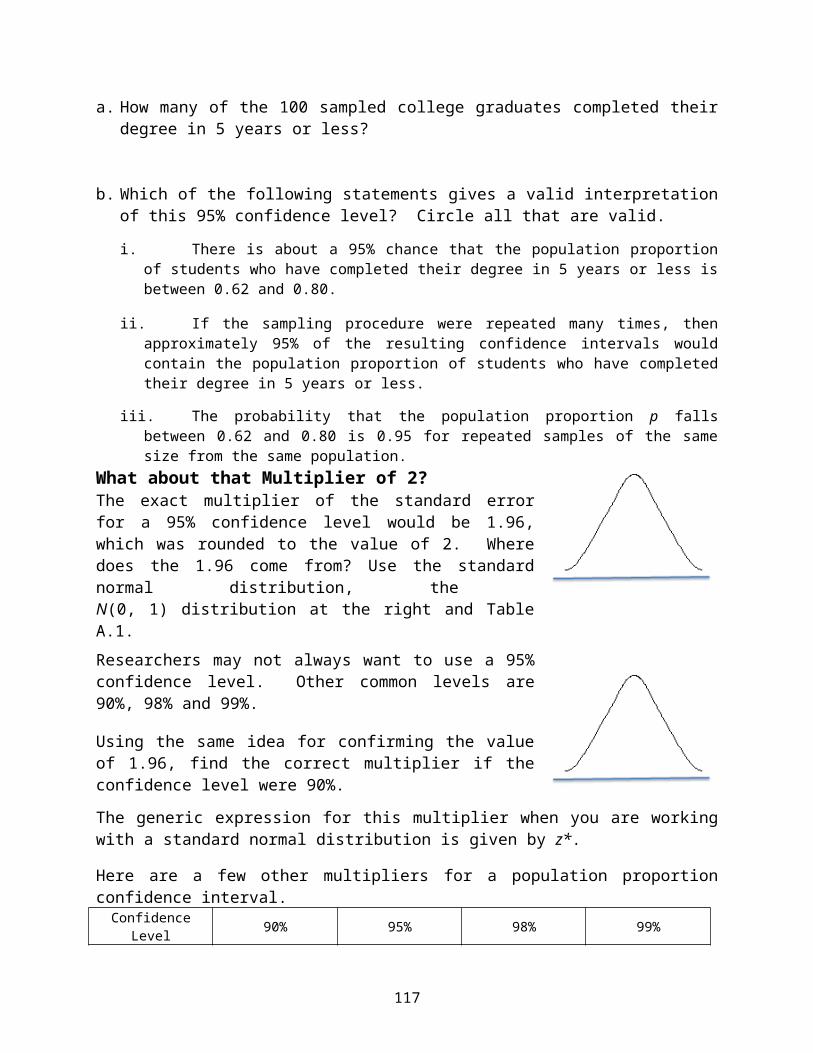
What can we say about the distribution of the sample mean?Distribution of the Sample Mean – Main ResultsLet = mean for the population of interest and = standard deviation for the that population.Let x = the sample mean for a random sample of size n.

If all possible random samples of the same size n are taken and x is computed for each, then …

The average of all of the possible sample mean values is equal to _____________________.

Thus the sample mean is an __________________ estimator of the population mean.

The standard deviation of all of the possible sample mean values is equal to the original

population standard deviation divided by √n .

Standard deviation of the sample mean is given by: s.d.( x ) = σ√n

What about the shape of the sampling distribution? The first two bullets above provide what the mean and the standard deviation are for the possible sample mean values. The final two bullets tell us that the shape of the distribution will be (approximately) normal.

If the parent (original) population has a normal distribution,then the distribution of the possible values of x , the sample mean, is normal.

If the parent (original) population is not necessarily normally distributedbut the sample size n is large, then the distribution of the possible values of x , the sample mean is approximately normal.

Original Population

Sample Mean Population

Take a random sample of ANY size n and compute the sample mean.

Original Population

Sample Mean Population

Take a random sample of size n where n is LARGE, and compute the sample mean.

118

This last result is called the .

The C in CLT is for CENTRAL. The CLT is an important or central result in statistics. As it turns out, many normal curve approximations for various statistics are really applications of the CLT. The Stat 250 formula card summarizes distribution of a sample mean as follows:

Try It! SRT Test ScoresA particular test for measuring various aspects of verbal memory is known as the Selective Reminding Task (SRT) test. It is based on hearing, recalling, and learning 12 words presented to the client. Scores for various aspects of verbal memory are combined to give an overall score. Let X represent overall score for 20-year-old females. Such scores are normally distributed with a mean of 126 and a standard deviation of 10.

a. What is the probability that a randomly selected 20-year-old female will have a score above 134?

b. A random sample of 9 such females will be selected. What is the probability that all nine will score below 134?

c. A random sample of 9 such females will be selected. What is the probability that their sample mean score will be above 134?

119

Try It! Actual Flight TimesSuppose the random variable X represents the actual flight time (in minutes) for Delta Airlines flights from Cincinnati to Tampa follows a uniform distribution over the range of 110 minutes to 130 minutes.

a. Sketch the distribution for X (include axes labels and some values on the axes).

b. Suppose we were to repeatedly take a random sample of size 100 from this distribution and compute the sample mean for each sample. What would the histogram of the sample mean values look like? Provide a smoothed out sketch of the distribution of the sample mean, include all details that you can.

Try It! True or FalseDetermine whether each of the following statements is True or False. A true statement is always true. Clearly circle your answer.

a. The central limit theorem is important in statistics because for a large random sample, it says the sampling distribution of the sample mean is approximately normal.

True False

b. The sampling distribution of a parameter is the distribution of the parameter value if repeated random samples are obtained.

True False

120

More on the Standard Deviation of X

The standard deviation of the sample mean is given by: s.d.( x ) = σ√n

This quantity would give us an idea about how far apart a sample mean x and the true population mean are expected to be on average.

We can interpret the standard deviation of the sample mean as approximately the average distance of the possible sample mean values (for repeated samples of the same size n) from the true population mean

Note: If the sample size increases, the standard deviation decreases, which says the possible sample mean values will be closer to the true population mean (on average).

The s.d.(x ) is a measure of the accuracy of the process of using a sample mean to estimate the

population mean. This quantity σ√n does not tell us exactly how far away a particular observed

x value is from

In practice, the population standard deviation is rarely known, so the sample standard deviation s is used. As with proportions, when making this substitution we call the result the

standard error of the mean s.e.(x ) = s

√n . This terminology makes sense, because this is a measure of how much, on average, the sample mean is in error as an estimate of the population mean.

Standard error of the sample mean is given by: s.e.(x ) = s

√nThis quantity is an estimate of the standard deviation of x .

So we can interpret the standard error of the sample mean as estimating, approximately, the average distance of the possible x values (for repeated samples of the same size n) from the true population mean Moreover, we can use this standard error to create a range of values that we are very confident will contain the true population mean namely, x(few)s.e.(x ). This is the basis for confidence interval for the population mean discussed in Part 2.

121

Preparing for Statistical Inference: Standardized StatisticsIn our SRT Test Scores and Actual Flight Times examples earlier, we have already constructed and used a standardized z-statistic for a sample mean.

z =

x−μσ

√n has (approximately) a standard normal distribution N(0,1).

Dilemma = _____________________________________

If we replace the population standard deviation with the sample standard deviation s, then x−μs√n won’t be approximately N(0,1); instead it has a _______________________

Student’s t-DistributionA little about the family of t-distributions ...

They are symmetric, unimodal, centered at 0. They are flatter with heavier tails compared to the N(0,1) distribution. As the degrees of freedom (df) increases ... the t distribution approaches the N(0,1)

distribution. We can still use the ideas about standard scores for a frame of reference. Tables A.2 and A.3 summarize percentiles for various t-distributions

From Utts, Jessica M. and Robert F. Heckard. Mind on Statistics, Fourth Edition. 2012. Used with permission.

We will see more on t-distributions when we do inference about population mean(s).

122

Every Statistic has a Sampling Distribution

The sampling distribution of a statistic is the distribution of possible values of the statistic for repeated samples of the same size from a population.

So far we have discussed the sampling distribution of a sample proportion, the sampling distribution of the difference between two sample proportions, and the sampling distribution of the sample mean. In all cases, under specified conditions the sampling distribution was approximately normal.

Every statistic has a sampling distribution, but the appropriate distribution may not always be normal, or even be approximately bell-shaped.

You can construct an approximate sampling distribution for any statistic by actually taking repeated samples of the same size from a population and constructing a histogram for the values of the statistic over the many samples.

Additional NotesA place to … jot down questions you may have and ask during office hours, take a few extra notes, write out an extra problem or summary completed in lecture, create your own summary about these

concepts.

123

124

Stat 250 Gunderson Lecture Notes7: Learning about a Population Mean

Part 2: Confidence Interval for a Population Mean

Do not put faith in what statistics say until you have carefully considered what they do not say. --William W. Watt

Earlier we studied confidence intervals for estimating a population proportion and the difference between two population proportions. Recall it is important to understand how to interpret an interval and how to interpret what the confidence level really means.

The interval provides a range of reasonable values for the parameter with an associated high level of confidence. For example we can say, “We are 95% confident that the proportion of Americans who do not get enough sleep at night is somewhere between 0.325 to 0.395, based on a random sample of n = 935 American adults.

The 95% confidence level describes our confidence in the procedure we used to make the interval. If we repeated the procedure many times, we would expect about 95% of the intervals to contain the population parameter.

Confidence Interval for a Population Mean Consider a study on the design of a highway sign. A question of interest is: What is the mean maximum distance at which drivers are able to read the sign? A highway safety researcher will take a random sample of n = 16 drivers and measure the maximum distances (in feet) at which each can read the sign.

Population parameter μ = _________ mean maximum distance to read the sign for ________________

Sample estimate x = _________ mean maximum distance to read the sign for ________________

But we know the sample estimate x may not equal μ , in fact, the possible x values vary from sample to sample. Because the sample mean is computed from a random sample, then it is a random variable, with a probability distribution.Sampling Distribution of the sample mean

If x is the sample mean for a random sample of size n, and either the original population of responses has a normal model or the sample size is large enough, the distribution of the sample mean is (approximately)

125

So the possible x values vary normally around μ with a standard deviation of σ√n . The

standard deviation of the sample mean, σ√n , is roughly the average distance of the possible

sample mean values from the population mean μ . Since we don’t know the population standard deviation we will use the sample standard deviation s, resulting in the standard error of the sample mean.

Standard Error of the Sample mean

s.e.(x ) = where s = sample standard deviation

The standard error of x estimates, roughly, the average distance of the possible x values from The possible x values result from considering all possible random samples of the same size n from the same population.

So we have our estimate of the population mean, the sample mean x , and we have its standard error. To make our confidence interval, we need to know the multiplier.

Sample Estimate Multiplier x Standard error

The multiplier for a confidence interval for the population mean is denoted by t*, which is the value in a Student’s t distribution with df = n – 1 such that the area between –t and t equals the desired confidence level. The value of t* will be found using Table A.2. First let’s give the formal result.

One-sample t Confidence Interval for

x±t ¿s .e .( x )where t∗¿ ¿ is an appropriate value for a t(n – 1) distribution.

This interval requires we have a random sample from a normal population. If the sample size is large (n > 30), the assumption of normality is not so crucial and the result is approximate.

Important items: be sure to check the conditions know how to interpret the confidence interval be able to explain what the confidence level of say 95% really means

126

Try It! Using Table A.2 to find t* (a) Find t∗¿ ¿ for a 90% confidence interval based on n = 12 observations.

(b) Find t∗¿ ¿ for a 95% confidence interval based on n = 30 observations.

(c) Find t∗¿ ¿ for a 95% confidence interval based on n = 54 observations.

(d) What happens to the value of t∗¿ ¿ as the sample size (and thus the degrees of freedom) gets larger?

From Utts, Jessica M. and Robert F. Heckard. Mind on Statistics, Fourth

Edition. 2012. Used with permission.

127

Try It! Confidence Interval for the Mean Maximum DistanceRecall the study on the design of a highway sign. The researcher wanted to learn about the mean maximum distance at which drivers are able to read the sign. The researcher took a random sample of n = 16 drivers and measured the maximum distances (in feet) at which each can read the sign. The data are provided below.

440 490 600 540 540 600 240 440360 600 490 400 490 540 440 490

a. Verify the necessary conditions for computing a confidence interval for the population mean distance. We are told that the sample was a random sample so we just need to check if a normal model for the response ‘max distance’ for the population is reasonable.

All images

Maximum Distance (in feet)

625575525475425375325275225

Cou

nt 5

4

3

2

1

0

Max

imum

Dis

tanc

e 700

650

600

550

500

450

400

350

300

250

200

Comments:Normal Q-Q Plot of DISTANCE

Observed Value

700600500400300200

Exp

ecte

d N

orm

al V

alue

700

600

500

400

300

128

440 490 600 540 540 600 240 440360 600 490 400 490 540 440 490

b. Compute the sample mean maximum distance and the standard error (without the outlier).

c. Use a 95% confidence interval to estimate the population mean maximum distance at which all drivers can read the sign. Write a paragraph that interprets this interval and the confidence level.

Using R Commander we would use the Single-Sample t-Test to produce the following results. Both the confidence interval and a test of hypotheses will be provided. We will discuss the hypothesis testing for a mean difference in Part 3.

One Sample t-test

data:  MaxDistt = 20.1005, df = 15, p-value = 2.934e-12alternative hypothesis: true mean is not equal to 095 percent confidence interval: 430.2184 532.2816sample estimates:

129

mean of x   481.25

130

Additional NotesA place to … jot down questions you may have and ask during office hours, take a few extra notes, write out an extra problem or summary completed in lecture, create your own

summary about these concepts.

131

Stat 250 Gunderson Lecture Notes7: Learning about a Population Mean

Part 3: Testing about a Population Mean

Introduction to Hypothesis Tests for Means

We have already been introduced us to the logic and steps of hypothesis testing for learning about a population proportion and for the difference between two population proportions. Recall the big idea that we declare “statistical significance” and reject the null hypothesis if the p-value is less than or equal to the significance level Now we will extend these ideas to testing about means, focusing first on hypothesis testing about a single population mean.

A few notes: Hypotheses and conclusions apply to the larger population(s) represented by the sample(s). And if the distribution of a quantitative variable is highly skewed, we should consider analyzing the median rather than the mean. Methods for testing hypotheses about medians are a special case of nonparametric methods, which we will not cover in detail, but do exist as the need arises.

Next let’s review the Basic Steps in Any Hypothesis Test.

Step 1: Determine the null and alternative hypotheses.The hypotheses are statements about the population(s), not the sample(s). The null hypothesis defines a specific value of a population parameter, called the null value.

Step 2: Verify necessary data conditions, and if met, summarize the data into an appropriate test statistic.

A relevant statistic is calculated from sample information and summarized into a “test statistic.” We measure the difference between the sample statistic and the null value using the standardized statistic:

Sample statistic – Null value (Null) standard error

For hypotheses about proportions (with large sample sizes), the standardized statistic is called a

______________ and the _______________________ is used to find the p-value.

For hypotheses about means, the standardized statistic is called a ______________ and the _______________________ is used to find the p-value.

Step 3: Assuming the null hypothesis is true, find the p-value.

A p-value is computed based on the standardized “test statistic.” The p-value is calculated by temporarily assuming the null hypothesis to be true and then calculating the probability that the test statistic could be as large in magnitude as it is (or larger) in the direction(s) specified by the alternative hypothesis.

132

Step 4: Decide if the result is statistically significant based on the p-value.

Based on the p-value, we either reject or fail to reject the null hypothesis. The most commonly used criterion (level of significance) is that we reject the null hypothesis when the p-value is less than or equal to the significance level (generally 0.05). In many research articles, p-values are simply reported and readers are left to draw their own conclusions. Remember that a p-value measures the strength of the evidence against the null hypothesis and the smaller the p-value, the stronger the evidence against the null (and for the alternative).

The Beauty of p-values: Suppose the significance level is set at 5% for testing H0: status quo versus Ha: the “new theory”.

If p-value is… Statistical Decision Feasible Conclusion about the “New Theory”

0.462 Fail to Reject H0

0.063 Fail to Reject H0

0.041 Reject H0

0.003 Reject H0

Step 5: Report the conclusion in the context of the situation.

The decision is to reject or fail to reject the null hypothesis, but the conclusion should go back to the original question of interest being asked. It should be stated in terms of the particular scenario or situation.

Testing Hypotheses about One Population Mean We have one population and a response that is quantitative. We wish to test about the value of the mean response for the population The data are assumed to be a random sample. The response is assumed to be normally distributed for the population (but if the sample size is large, this condition is less crucial).

Step 1: Determine the null and alternative hypotheses.

1. H0: versus Ha:

2. H0: versus Ha:

3. H0: versus Ha:

133

Step 2: Verify necessary data conditions, and if met, summarize the data into an appropriate test statistic.

How would you check the conditions as stated in the scenario above?

Test statistic = Sample statistic – Null value Standard error

If H0 is true, this test statistic has a ______________ distribution.

Step 3: Assuming the null hypothesis is true, find the p-value.Steps for finding a p-value …

Draw the distribution for the test statistic under H0

For t tests it will be a t-distribution with a certain df. Locate the observed test statistic value on the axis. Shade in the area that corresponds to the p-value. Look at the alternative hypothesis for the direction of extreme. Use the appropriate table to find (bounds for) the p-value.

For t tests we use Table A.3.

Step 4: Decide whether or not the result is statistically significant based on the p-value.The level of significance is selected in advance. We reject the null hypothesis if the p-value is less than or equal to In this case, we say the results are statistically significant at the level

Step 5: Report the conclusion in the context of the situation.Once the decision is made, a conclusion in the context of the problem can be stated.

From the Stat 250 formula card:Population MeanParameter

Statistic x

Standard Error

nsx )(s.e.

One-Sample t-Test

nsx

xx

t 00

)(s.e.

df = n – 1

134

From Utts, Jessica M. and Robert F. Heckard. Mind on Statistics, Fourth Edition. 2012. Used with permission.

135

Try It! Using Table A.3 to find a p-value for a one-sided testWe are testing H0: = 0 versus Ha: > 0 with n = 15 observations and the observed test statistic is 97.1t

Draw the distribution for the test statistic under H0

Locate the observed test statistic value on the axis.

Shade in the area that corresponds to the p-value.Look at the alternative hypothesis for the direction of extreme.

Use the appropriate table to find (bounds for) the p-value.For t tests we will use Table A.3.

Is the value of 97.1t significant at the 5% level? __________

At the 1% level? _________

Try It! Using Table A.3 to find a p-value for a two-sided testWe are testing H0: = 64 versus Ha: ≠ 64 with n = 30 observations and the observed test statistic is 12.1t . How would you report the p-value for this test?

136

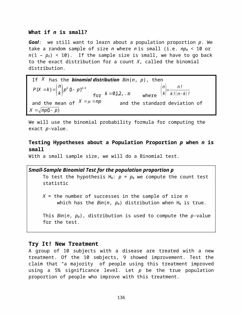
Try It! Classical Music A researcher wants to test if HS students complete a maze more quickly while listening to classical music. For the general HS population, the time to complete the maze is assumed to follow a normal distribution with a mean of 40 seconds. Use a 5% significance level.

Define the parameter of interest: Let represent…

State the hypotheses: H0:

Ha:

A random sample of 100 HS students are timed while listening to classical music. The mean time was 39.1 seconds and the standard deviation was 4 seconds. Conduct the test.

Are the results statistically significant at the 5% level? ______________________State the conclusion at the 5% level in terms of the problem.

Comment about the assumptions required for this test to be valid:

137

Try It! Calcium Intake A bone health study looked at the daily intake of calcium (mg) for 38 women. They are concerned that the mean calcium intake for the population of such women is not meeting the RDA level of 1200 mg, that is, the population mean is less than the 1200 mg level. They wish to test this theory using a 5% significance level.a. State the hypotheses about the mean calcium intake for the population of such women.

H0: ________________________ versus Ha: _____________________

Summary StatisticsMean Std. Dev (s) Sample Size (n) Std. Error926.03 427.23 38 69.31

Below are the t-test results generated using R Commander and selecting Statistics > Means > Single-Sample T Test. A test value of 1200 was entered and the correct direction for the alternative hypothesis was selected. Notice that a 95% one-sided confidence bound is provided since our test alternative was one-sided to the left. If you wanted to also report a regular 95% confidence interval, you would run a two-sided hypothesis test in R.

One Sample T Resultst df p-value 95% CI Lower 95% CI Upper

-3.953 37 0.000165 *** 1043.16

b. Interpret the Std. Error of the mean (SEM):

c. Give the observed test statistic value: _____ = ______________Interpret the this value in terms of a difference from the hypothesized mean of 1200.

d. Sketch a picture of the p-value in terms of an area under a distribution.

e. Give the p-value and the conclusion using a 5% significance level.

138

The Relationship between Significance Tests and Confidence IntervalsEarlier we discussed the using of confidence intervals to guide decisions. A confidence interval provides a range of plausible (reasonable) values for the parameter. The null hypothesis gives a null value for the parameter. So: If this null value is one of the “reasonable” values found in the confidence interval,

the null hypothesis would not be rejected. If this null value was not found in the confidence interval of acceptable values for the

parameter, then the null hypothesis would be rejected.

Notes:(1) The alternative hypothesis should be two-sided. However, sometimes you can reason

through the decision for a one-sided test.

(2) The significance level of the test should coincide with the confidence level (e.g. = 0.05 with a 95% confidence level). However, sometimes you can still determine the decision if these do not exactly correspond (see part (c) of the next Try It!).

(3) This relationship holds exactly for tests about a population mean or difference between two population means. In most cases, the correspondence will hold for tests about a population proportion or difference between two population proportions.

Try It! Time Spent Watching TVA study looked at the amount of time that teenagers are spending watching TV. Based on a representative sample, the 95% confidence interval for mean amount of time (in hours) spent watching TV on a weekend day was given as: 2.6 hours ± 2.1 hours. So the interval goes from 0.5 hours to 4.7 hours.

a. Test H0: = 5 hours versus Ha: ≠ 5 hours at .05.0 Reject H0 Fail to reject H0 Can't tellWhy?

b. Test H0: = 4 hours versus Ha: ≠ 4 hours at .05.0 Reject H0 Fail to reject H0 Can't tellWhy?

c. Test H0: = 4 hours versus Ha: ≠ 4 hours at 01.0 Reject H0 Fail to reject H0 Can't tellWhy?

d. Test H0: = 4 hours versus Ha: ≠ 4 hours at 10.0

Reject H0 Fail to reject H0 Can't tellWhy?

139

Try It! MBA grads Salaries“It’s a good year for MBA grads” was the title of an article. One of the parameters of interest was the population mean expected salary, (in dollars). A random sample of 1000 students who finished their MBA this year (from 129 business schools) resulted in a 95% confidence interval for of (83700, 84800).

a. What is the value of the sample mean? Include your units.

b. For each statement determine if it is true or false. Clearly circle your answer.

If repeated samples of 1000 such students were obtained, we would expect 95% of the resulting intervals to contain the population mean.

True False

There is a 95% probability that the population mean lies between $83,700 and $84,800.

True False

c. The expected average earnings for such graduates in past year was $76,100. Suppose we wish to test the following hypotheses at the 10% significance level:

H0: = 76100 versus Ha: ≠ 76100.

Our decision would be: Fail to reject H0 Reject H0 can’t tellBecause …

d. Several plots of the expected salary data were constructed to help verify some of the data conditions. A qq-plot is provided for checking the assumption that the response is normally distributed. This plot shows some departure from a straight line with a positive slope. Is this cause for concern that inference based on our confidence interval and hypothesis test would not be valid? Explain.

140

Additional NotesA place to … jot down questions you may have and ask during office hours, take a few extra notes, write out an extra problem or summary completed in lecture, create your

own summary about these concepts.

141

Stat 250 Gunderson Lecture Notes8: Learning about a Population Mean Difference

Part 1: Distribution for a Sample Mean of Paired Differences

The Paired Data ScenarioAn important special case of a single mean of a population occurs when two quantitative variables are collected in pairs, and we desire information about the difference between the two variables. Here are some ways that paired data can occur:

Each person or unit is measured twice. The two measurements of the same characteristic or trait are made under different conditions. An example is measuring a quantitative response both before and after treatment.

Similar individuals or units are paired prior to an experiment. During the experiment, each member of a pair receives a different treatment. The same quantitative response variable is measured for all individuals.

For paired data designs, it is the differences that we are interested in examining. By focusing on the differences we again have just one sample of observations (the differences). Sometimes you may see a “d” in the subscript of the mean to represent the mean of the population of differences: d; and the data may be represented generically as: d1 , d2 , . .. , dn .

Sampling Distribution for the Sample Mean of Paired DifferencesThe sampling distribution results for the mean of paired differences is really the same as that for a regular sample mean. Since the measurements are differences, the sample mean of the data, x , is just written as d , to emphasize that this is a paired design.

Freshmen WeightA study was conducted to learn about the average weight gain in the first year of college for students. A sample of 60 students resulted in an average weight gain of 4.2 pounds (over the first 12 weeks of college).

Population =

Parameter =

Sample =

Statistic =

Can anyone say how close this observed sample mean difference d of 4.2 pounds is to the true population mean difference d? __________ If we were to take another random sample of the same size, would we get the same value for the sample mean difference? ________________. So what are the possible values for the sample mean difference d if we took many random samples of the same size from this population? What would the distribution

142

of the possible d values look like? What can we say about the distribution of the sample mean difference?

143

Distribution of the Sample Mean Difference – Main Results

Let d = mean of the differences in the population of interest.Let d = standard deviation for the differences in the population of interest.Let d = the sample mean of the differences for a random sample of size n.

If the population of differences is normal (bell-shaped), and a random sample of any size is obtained, then the distribution of the sample mean difference d is also normal, with a

mean of d and a standard deviation of s .d .( d )=

σd

√n . If the population of differences is not normal (bell-shaped), but a large random sample of

size n is obtained, then the distribution of the sample mean difference d is approximately

normal, with a mean of d and a standard deviation of s .d .( d )=

σd

√n .Notes: (1) An arbitrary level for what is ‘large’ enough has been 30. However, if any of the differences

are extreme outliers, it is better to have a larger sample size.(2) The standard deviation of d is a measure of the accuracy of the process of using a sample

mean difference to estimate the population mean difference.

s .d .( d )=

σd

√n(3) In practice, the population standard deviation d is rarely known, so the sample standard

deviation sd is used instead. When making this substitution we call the result a standard error.

Standard error of the sample mean difference is given by:

s.e.( d ) =

sd√n

We can interpret the standard error of the sample mean difference as estimating, approximately, the average distance of the possible d values (for repeated samples of the same size n) from the population mean difference d.

Moreover, we can use this standard error of the sample mean difference to produce a range of values that we are very confident will contain the population mean difference d, namely, d (a few)s.e.( d ). This is the basis for confidence interval for the population mean difference d, discussed in Part 2.

144

145

Looking ahead:

Do you think the ‘few’ in the expression d (a few)s.e.( d ) will be a z* value or a t* value?

What degrees of freedom will be used?

We will use the standard error of the sample mean difference to compute a standardized test statistic for testing hypotheses about the population mean difference d, namely,

Sample statistic – Null value. (Null) standard error

This is the basis for testing about a population mean difference covered in Part 3.

Looking ahead:

Do you think the standardized test statistic will be a z statistic or a t statistic?

What do you think will be the most common null value?

H0: d = _______

146

Additional NotesA place to … jot down questions you may have and ask during office hours, take a few extra notes, write out an extra problem or summary completed in lecture, create your own summary about these

concepts.

147

Stat 250 Gunderson Lecture Notes8: Learning about a Population Mean Difference

Part 2: Confidence Interval for a Population Mean of Paired Differences

Confidence Interval for the Population Mean of Paired Differences d

Recall that an important special case of a single mean of a population occurs when two quantitative variables are collected in pairs, and we desire information about the difference between the two variables. For paired data designs, it is the differences that we are interested in analyzing. By focusing on the differences we again have just one sample of observations (the differences) and are able to use the confidence interval for the population mean difference.

Notation:

Population Parameter: d = population mean difference

Data: d1 , d2 , . .. , dn

Sample Estimate: d = sample mean difference

Standard Error: s.e.( d ) =

sd√n (sd = standard deviation of the sampled differences)

We use the sample estimate and its standard error to form a confidence interval estimate for the parameter using the following form:

Sample Estimate Multiplier x Standard error

The multiplier used will depend on the confidence level, the sample size, and the type of parameter being estimated. In this case, since we are estimating a single population mean, the multiplier will be a t* value. Here is the summary for a paired data confidence interval:

One-sample t Confidence Interval for the Population Mean Difference d

d± t¿ s .e .( d )where t∗¿ ¿ is the appropriate value for a t(n – 1) distribution.

Note that n is the number of pairs, or the number of differences. This interval requires that the differences can be considered a random sample from a normal population. If the sample size is large, the assumption of normality is not so crucial and the result is approximate.

148

Try It! Changes in Reasoning ScoresDo piano lessons improve spatial-temporal reasoning of preschool children?Data: The change in reasoning score, after piano lessons - before piano lessons, with larger values indicating better reasoning, for a random sample of n = 34 preschool children.

2 5 7 -2 2 7 4 1 0 7 3 43 4 9 4 5 2 9 6 0 3 6 -13 4 6 7 -2 7 -3 3 4 4

(a) Display the data, summarize the distribution. These data were entered into R to produce the following histogram.

Some summary measures were obtained using R Commander and entered into the table:> numSummary(Dataset[,"ChangeReas"], statistics=c("mean", "sd", "IQR", + "quantiles"), quantiles=c(0,.25,.5,.75,1)) mean sd IQR 0% 25% 50% 75% 100% n 3.617647 3.055196 4 -3 2 4 6 9 34

Summary StatisticsMean diff (d) Std. Dev (sd) Sample size (n) Std. Error

3.62 3.06 34 0.52

(b) Give a 95% confidence interval for the population mean improvement in reasoning scores.

(c) What value is of particular interest to see whether or not it is in the interval?

Notes:1. Diff = after – before so …

2. Sample mean difference = ______

3. Normality of the response (the difference) for the population?

149

150

(d) A student in your class wrote the following interpretation about the 95% confidence level used in making the interval. Is it a correct interpretation? If not, update it to make it correct.

“If this study were repeated many times, we would expect 95% of the resulting confidence intervals to contain the sample mean improvement in reasoning scores.”

R Note: The differences were already computed and entered as the data. So to make a confidence interval with R Commander we would need to perform a single-sample t-Test on the differences (and leave the null hypothesis value the default of 0). Be sure the confidence level is the one you want, namely .95.

> with(Dataset, (t.test(ChangeReas, alternative='two.sided', mu=0.0, + conf.level=.95)))

One Sample t-test

data: ChangeReast = 6.9044, df = 33, p-value = 6.919e-08alternative hypothesis: true mean is not equal to 095 percent confidence interval: 2.551639 4.683655sample estimates:mean of x 3.617647

Paired T ResultsMean diff (d) df 95% CI Lower 95% CI Upper

3.62 33 2.55 4.68

If the before and after scores were entered into R, then we would use a paired t-test option. R would compute the differences for us and provide the confidence interval results. Details of the R steps for analyzing paired data can be found in your Lab Workbook.

151

152

Additional NotesA place to … jot down questions you may have and ask during office hours, take a few extra notes, write out an extra problem or summary completed in lecture, create your own summary about these

concepts.

153

Stat 250 Gunderson Lecture Notes8: Learning about a Population Mean Difference

Part 3: Testing about a Population Mean of Paired Difference

Testing Hypotheses about the Population Mean of Paired Differences d

An important special case of a single mean of a population occurs when two quantitative variables are collected in pairs, and we desire information about the difference between the two variables. For paired data designs, it is the differences that we are interested in analyzing. By focusing on the differences we again have just one sample of observations (the differences) and are able to perform a one-sample t-test on the differences.

The procedure for the significance test is really the same - the sample mean of the data, x , is just written as d , primarily to emphasize that this is a paired design with the differences being analyzed. The commonly used null hypothesis is that the population mean difference is d = 0.

Possible null and alternative hypotheses.

1. H0: versus Ha:

2. H0: versus Ha:

3. H0: versus Ha:

Note: The format of the alternative hypothesis depends on the research question of interest and the order in which the differences were taken.

Test Statistic and Conditions for the Test

Test statistic = Sample statistic – Null valueStandard error

If H0 is true, this test statistic has a _________________________ distribution.

We use this distribution to report the (bounds for the) p-value.

Conditions for the test: The difference is assumed to be normally distributed for the population (but if the sample size is large, this condition is less crucial). So you need to examine the differences graphically and assess if there are any extreme outliers or skewness in the differences. If so, either the sample size needs to be large or an alternative testing method may be required.

154

155

Try It! Knob TurningA study involved n=25 right-handed students and a device with two different knobs (right-hand thread and left-hand thread). The response of interest is the time it takes to move knob indicator a fixed distance. The question of interest is to assess if right-hand threads are easier to turn on average. Use a 5% significance level.

a. Why is this a paired design and how should randomization be used in the experiment?

b. State the hypotheses. H0: _________________versus Ha: _______________

Here are a few summaries of each set of responses separately and then of the paired data:Paired Samples Statistics

104.00 25 15.93 3.19117.44 25 27.26 5.45

RTHREADLTHREAD

Pair1

Mean N Std. DeviationStd. Error

Mean

Below are the t-test results generated using R Commander and selecting Statistics > Means > Paired T Test and the correct direction for the alternative hypothesis. Notice that a 95% one-sided confidence bound is provided since our test alternative was one-sided to the left. If you wanted to also report a regular 95% confidence interval, you would run a two-sided hypothesis test in R.

Summary StatisticsMean diff (d ) Std. Dev (sd) Sample size (n) Std. Error

-13.44 23.06 25 4.61

Paired T Resultst df p-value 95% CI Lower 95% CI Upper

-2.914 24 0.004 *** -5.55

c. Perform the test.

d. Which are assumptions required for performing the paired t-test? the turning times for the right-hand threaded knob are independent of the turning times

for the left-hand threaded knob. the turning times for the right-hand threaded knob are normally distributed. the difference in turning times (diff = RT – LT) is normally distributed.

156

Additional NotesA place to … jot down questions you may have and ask during office hours, take a few extra notes, write out an extra problem or summary completed in lecture, create your own summary about these

concepts.

157

158

Stat 250 Gunderson Lecture Notes9: Learning about the Difference in Population Means

Part 1: Distribution for a Difference in Sample Means

The Independent Samples ScenarioRecall that two samples are said to be independent samples when the measurements in one sample are not related to the measurements in the other sample. Independent samples are generated in a variety of ways. Some common ways:

Random samples are taken separately from two populations and the same response variable is recorded for each individual.

One random sample is taken and a variable is recorded for each individual, but then units are categorized as belonging to one population or another, e.g. male/female.

Participants are randomly assigned to one of two treatment conditions, such as diet or exercise, and the same response variable, such as weight loss, is recorded for each individual unit.

If the response variable is quantitative, a researcher might compare two independent groups by looking at the difference between the two means.

Sampling Distribution for the Difference in Two Sample MeansFamily Dinners and Teen StressA study was conducted to look at the relationship between the number of times a teen has dinner with their family and level of stress in the teen’s life. Teens were asked to rate the level of stress in their lives on a point scale of 0 to 100.

The researcher would like to estimate the difference in the population mean stress level for teens who have frequent family dinners (group 1) versus the population mean stress level for teens who have infrequent family dinners (group 2).

A Typical Summary of Responses for a Two Independent Samples ProblemPopulation Sample Size Sample Mean Sample Standard Deviation

1 Frequent 10 53.5 15.72 Infrequent 10 65.5 14.6

Let 1 be the population mean stress level for all teens who have frequent family dinners.

Let 2 be the population mean stress level for all teens who have infrequent family dinners.

We want to learn about 1 and 2 and how they compare to each other. We could estimate

the difference in population means 21 with the difference in the sample means 21 xx . Will it be a good estimate?

159

Can anyone say how close this observed difference in sample mean stress levels 21 xx of

-12 points is to the true difference in population means 21 ? _________

If we were to repeat this survey (with samples of the same sizes), would we get the same value for the difference in sample means? ___________________

Is a difference in the sample means of 12 points large enough to convince us that there is a real difference in the means for the populations of teens?

So what are the possible values for the difference in sample means 21 xx if we took many sets of independent random samples of the same sizes from these two populations? What would

the distribution of the possible 21 xx values look like?

What can we say about the distribution of the difference in two sample means?

Using results from how to handle differences of independent random variables and the results for the sampling distribution for a single sample mean, the sampling distribution of the

difference in two sample means 21 xx can be determined.

First recall that when working with the difference in two independent random variables: the mean of the difference is just the difference in the two means the variance of the difference is the sum of the variances

Next, remember that the standard deviation of a sample mean is

σ√n .

So what would the variance of a single sample mean be?

So let’s apply these ideas to our newest parameter of interest, the difference in two sample

means 21 xx .

Sampling Distribution of the Difference in Two (Indep) Sample Means

If the two populations are normally distributed (or sample sizes are both large enough),

Then 21 xx is (approximately)

160

161

Since the population standard deviations of 1 and 2 are generally not known, we will use the data to compute the standard error of the difference in sample means.

Standard Error of the Difference in Sample Means

2

22

1

21

21s.e.ns

ns

xx

where s1 and s2 are the two sample standard deviations

The standard error of 21 xx estimates, roughly, the average distance of the possible

21 xx values from The possible 21 xx values result from considering all possible independent random samples of the same sizes from the same two populations.

Moreover, we can use this standard error to produce a range of values that we are

very confident will contain the difference in the population means 21 , namely,

21 xx (a few)s.e.( 21 xx ). This is the basis for confidence interval for the difference in population means discussed in Part 2.

Looking ahead:Do you think the ‘few’ in the above expression will be a z* value or a t* value?What do you think will be the degrees of freedom?

We will use the standard error of the difference in the sample means to compute a standardized test statistic for testing hypotheses about the difference in the population means

21 , namely,Sample statistic – Null value. (Null) standard error

This is the basis for testing covered in Part 3.

Looking ahead: Do you think the standardized test statistic will be a z statistic or a t statistic?What do you think will be the most common null value used?

H0: 21 = _____________

162

163

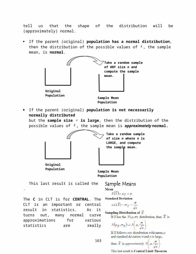
Stat 250 Gunderson Lecture NotesLearning about the Difference in Population Means

Part 2: Confidence Interval for a Difference in Population Means

Confidence Interval for the Difference in Two Population Means

General (Unpooled) Approach We have two populations or groups from which independent samples are available, (or

one population for which two groups can be formed using a categorical variable). The response variable is quantitative and we are interested in comparing the means for

the two populations.

A Typical Summary of the Responses for a Two Independent Samples Problem:Population Sample Size Sample Mean Sample Standard Deviation

1 1n 1x 1s2 2n 2x 2s

Let 1 be the mean response for the first population and 2 be the mean response for the second population.

Parameter of interest: the difference in the population means 21 .

Sample estimate: the difference in the sample means 21 xx .

Standard error:

2

22

1

21

21s.e.ns

ns

xx where s1 and s2 are the sample standard deviations.

So we have our estimate of the difference in the two population means, namely 21 xx , and we have its standard error. To make our confidence interval, we need to know the multiplier. The multiplier t* is a t-value such that the area between –t* and t* equals the desired confidence level. The degrees of freedom for the t-distribution will depend on whether we use an ugly formula (used by software packages) or we use a conservative “by-hand” approach.

General Two Independent-Samples t Confidence Interval for 1 - 2

)s.e.( 21*

21 xxtxx

where

2

22

1

21

21s.e.ns

ns

xx and *t is the appropriate value for a t-distribution, and the

df can be found using an approximation or conservatively as df = smaller of (n1 – 1 or n2 – 1)

This interval requires we have independent random samples from normal populations. If the sample sizes are large (both > 30), the assumption of normality is not so crucial and the result is approximate.

164

The Pooled Approach

If we can further assume the population variances are (unknown but) equal, then there is a procedure for which the t* multiplier is easier to find using an exact (not approximate) t-distribution. It involves pooling the sample variances for an overall estimate and updating the standard error accordingly.

It sometimes may be reasonable to assume that the measurements in the two populations have the same variances …

so that ____________________ where _____ denotes the common population variance.

Since both sample variances would be estimating the common population variance, it would make sense to combine or pool the two sample variances together to form an overall estimate.

Pooled standard deviation: sp=√(n1−1) s1

2+(n2−1)s22

n1+n2−2 Notes:(1) Each sample variance is weighted by the corresponding degrees of freedom.

So a larger sample size will result in a larger weight for that sample variance.(2) The denominator gives the total degrees of freedom:

df =

Replacing the individual standard deviations s1 and s2 with the pooled version sp in the formula

for the standard error leads to the pooled standard error of 21 xx is given by:

Pooled s.e.( 21 xx ) =

Pooled Two Independent-Samples t Confidence Interval for 1 - 2

( x1− x2)±t¿ ( pooled s .e .( x1− x2 ))

where pooled s .e . ( x1− x2 )=s p√ 1

n1+ 1n2

and sp=√(n1−1) s1

2+(n2−1)s22

n1+n2−2 and *t is the appropriate value for a t(n1 + n2 – 2) distribution.

165

This interval requires we have independent random samples from normal populations with equal population variances. If the sample sizes are large(both>30), the assumption of normality is not so crucial and the result is approximate.

166

Notes:

(1) Some computer software packages will provide results for both the unpooled and the pooled two independent samples t procedures automatically. Others, such as R, will require you to explore the data in appropriate ways to help decide which method you wish to use up front as you request the analysis.

(2) First compare the sample standard deviations. If the sample standard deviations are similar, the assumption of common population variance is reasonable and the pooled procedure can be used. If the sample sizes happen to be the same, the pooled and unpooled standard errors are equal anyway. The advantage for the pooled version is that finding the df is simpler.

(3) A graphical tool to help assess if equal population variances is reasonable is side-by-side boxplots. If the lengths of the boxes (the IQRs) and overall ranges between the two groups are very different, the pooled method may not be reasonable.

(4) Some computer software also provide or allow you to produce first the results of a Levene’s test for assessing if the population variances can be assumed equal.

The null hypothesis for this test is that the population variances are equal. So a small p-value for Levene’s test would lead to rejecting that null hypothesis and concluding that the pooled procedure should not be used.

Often a significance level of 10% is used for this condition checking. Your lab workbook provides more details about Levene’s test. We will see Levene’s test results in some of our examples ahead.

Bottom-line: Pool if reasonable; but if the sample standard deviations are not similar, we have the unpooled procedure that can be used.

Try It! Comparing Stress Levels Scores

A study was conducted to look at the relationship between the number of times a teen has dinner with their family and level of stress in the teen’s life. Teens were asked to rate the level of stress in their lives on a point scale of 0 to 100.

The researcher would like to estimate the difference in the population mean stress level for teens who have frequent family dinners (group 1) versus the population mean stress level for teens who have infrequent family dinners (group 2). Here is a partial listing of the data in

167

R. Note there are two Dinner Group variables, one is numerical (as was in the original data set) and the other is categorical (needed for R).Some descriptive summaries, side-by-side boxplots, and Levene’s Test results are provided first.

Population Sample Size Sample Mean Sample Standard Deviation1 Frequent 10 53.5 15.7

2 Infrequent 10 65.5 14.6

> with(Dataset, tapply(stresslevel, group, var, na.rm=TRUE))

Frequent Infrequent 244.7222 213.6111

> leveneTest(stresslevel ~ group, data=Dataset, center="mean")Levene's Test for Homogeneity of Variance (center = "mean")

Df F value Pr(>F)group 1 0.3958 0.5372 18

a. One of the assumptions for the pooled two independent samples confidence interval to be valid is that the two populations (from which we took our samples) have the same standard deviation. Look at the two sample standard deviations, the boxplots, and the Levene's test result. Does the assumption seem to hold (at the 10% level)? Explain.

b. Give a 95% confidence interval for the difference in the population mean stress levels, that is, for 1 - 2. Show all work.

168

c. Based on the interval, does there appear to be a difference in the mean stress levels for the two populations? Explain.

We could use R Commander to generate the t-test output using Statistics > Means > Independent-Samples T Test. Under the Options tab, since we want a (two-sided) confidence interval, we select two-sided for the alternate direction. Set the confidence level and the appropriate setting for “Allow equal variances?”

> t.test(stresslevel~group, alternative='two.sided', conf.level=.95, + var.equal=TRUE, data=Dataset)

Two Sample t-test

data: stresslevel by groupt = -1.7725, df = 18, p-value = 0.09323alternative hypothesis: true difference in means is not equal to 095 percent confidence interval: -26.223309 2.223309sample estimates: mean in group Frequent mean in group Infrequent 53.5 65.5

169

Try It! Stroop’s Word Color Test In Stroop’s Word Color Test, words that are color names are shown in colors different from the word. For example, the word red might be displayed in blue. The task is to correctly identify the display color of each word; in the example just given the correct response would be blue.

Gustafson and Kallmen (1990) recorded the time needed to complete the Color Test for n = 16 individuals after they had consumed alcohol and for n = 16 other individuals after they had consumed a placebo drink flavored to taste as if it contained alcohol. Each group was balanced with 8 men and 8 women.

In the alcohol group, the mean completion time was 113.75 seconds and standard deviation was 22.64 seconds. In the placebo group, the mean completion time was 99.87 seconds and standard deviation was 12.04 seconds.

Group Sample size Sample mean Sample standard deviation1 = alcohol 16 113.75 22.642 = placebo 16 99.87 12.04

We can assume that the two samples are independent random samples, that the model for completion time is normal for each population.a. What graph(s) would you make to check the normality condition? Be specific.

b. How did the two groups compare descriptively?

c. Which procedure? Pooled or unpooled? Why?

d. Calculate a 95% confidence interval for the difference in population means.

e. Based on the confidence interval, can we conclude that the population means for the two groups are different? Why or why not?

170

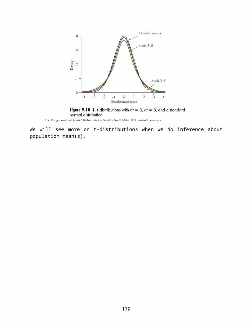
What if? Suppose the researchers Gustafson and Kallmen were convinced (based on past results) that the underlying population variances were equal, so they prefer that a pooled confidence interval be constructed. The estimate of the common population standard deviation would be:

sp=√(n1−1) s12+(n2−1)s2

2

n1+n2−2=√(16−1) (22.64 )2+(16−1) (12. 04 )2

16+16−2=√328 .77=18 .13

The pooled standard error for the difference in the two sample means would be:

pooled s .e . ( x1− x2 )=s p√ 1n1

+ 1n2

=18. 13√ 116

+ 116

=6 . 41

which is the same as the unpooled standard error since the sample sizes were equal. The t* multiplier would be based on df = 16 + 16 – 2 = 30, so t* = 2.04 (from Table A.2).

The 95% Pooled Confidence Interval would be:

( x1− x2)±t¿ (pooled s .e .( x1− x2 )) (13.88) (2.04)(6.41) 13.88 13.08 (0.80, 26.96)

This interval still does not include 0, so the same decision would be made; however, the interval is a bit narrower. In this example, the unpooled interval may be a bit conservative (wider) but the evidence is still strong to state the two population means appear to differ.

Stat 250 Formula Card

171

172

Stat 250 Gunderson Lecture Notes9: Learning about the Difference in Population Means

Part 3: Testing about a Difference in Population Means

Testing Hypotheses about the Difference in Two Population Means

We have two populations or groups from which independent samples are available, (or one population for which two groups can be formed using a categorical variable).

The response variable is quantitative and we are interested in testing hypotheses about the means for the two populations.

A Typical Summary of the Responses for a Two Independent Samples Problem:Population Sample Size Sample Mean Sample Standard Deviation

1 1n 1x 1s2 2n 2x 2s

Let 1 be the mean response for the first population and 2 be the mean response for the second population.

Parameter of interest: the difference in the population means 21 .

Sample estimate: the difference in the sample means 21 xx .

Standard error:

2

22

1

21

21s.e.ns

ns

xx

where s1 and s2 are the two sample standard deviations

Pooled standard error: pooled s.e . ( x1− x2 )=s p√ 1

n1+ 1n2

where sp=√(n1−1) s1

2+(n2−1)s22

n1+n2−2

Recall there are two methods for conducting inference for the difference between two population means for independent samples – the General (Unpooled) Case and the Pooled Case. Both require we have independent random samples from normal populations (but if the

173

sample sizes are large, the assumption of normality is not so crucial). Both will result in a t-test statistic, but the standard error used in the denominator differ as well as the degrees of freedom used for computing the p-value using a t-distribution.

Here is the summary for these two significance tests: Possible null and alternative hypotheses.

1. H0: versus Ha:

2. H0: versus Ha:

3. H0: versus Ha:

Test statistic = Sample statistic – Null value Standard error

Recall the guidelines to assess which version to use:(1) First compare the sample standard deviations. If the sample standard deviations are

similar, the assumption of common population variance is reasonable and the pooled procedure can be used.

(2) A graphical tool to help assess if equal population variances is reasonable is side-by-side boxplots. If the lengths of the boxes (the IQRs) and overall ranges between the two groups are very different, the pooled method may not be reasonable.

(3) Examine the results of a Levene’s test for assessing if the population variances can be assumed equal. The null hypothesis for this test is that the population variances are equal. So a small p-value for Levene’s test would lead to rejecting that null hypothesis and concluding that the pooled procedure should not be used.

174

Bottom-line: Pool if reasonable; but if the sample standard deviations are not similar, we have the unpooled procedure that can be used.

Try It! Effect of Beta-blockers on pulse rateDo beta-blockers reduce the pulse rate? In a study of heart surgery, 60 subjects were randomly divided into two groups of 30. One group received a beta-blocker while the other group was given a placebo. The pulse rate at a particular time during the surgery was measured. The results are given below.

Group Sample size Sample mean Sample standard deviation1=beta-blockers 30 65.2 7.8

2=placebo 30 70.3 8.4

a. State the hypotheses to assess if beta-blockers reduce pulse rate on average.

H0: ____________________ versus Ha: _______________________

b. Which test will you perform – the pooled or unpooled test? Explain.

c. Perform the t-test. Show all steps. Are the results significant at a 5% level?

175

Try It! Does the Drug Speed Learning? In an animal-learning experiment, a researcher wanted to assess if a particular drug speeds learning. One group of 5 rats (Group 1 = control) is required to learn to run a maze without use of the drug, whereas a second independent group of 8 rats (Group 2 = experimental) is administered the drug. The running times (time to complete the maze) for the rats in each group were entered into R.

Summary Statistics

Group Mean Std. Dev Sample Size General Std. Error

Pooled Std. Error

Control 46.80 3.42 52.28 2.47

Experimental 38.38 4.78 8

> leveneTest(stresslevel ~ group, data=Dataset, center="mean")Levene's Test for Homogeneity of Variance (center = "mean") Df F value Pr(>F)group 1 1.09 0.32 11

Conduct the test to address the theory of the researcher (state the null and alternate hypotheses, report the test statistic, p-value, and state your decision and conclusion at the 5% level of significance).

H0: _______________________ Ha: _______________________

Test statistic: ___________________ p-value: ________________________

Decision: (circle one) Fail to reject H0 Reject H0

Thus …

Two Sample T Resultst df p-value

Unpooled 3.70 10.653 0.002Pooled 3.41 11 0.003

176

Try It! Eat that Dark Chocolate An Ann Arbor News article entitled: Dark Chocolate may help blood flow, reported the results of a study in which researchers fed a small 1.6-ounce bar of dark chocolate to each of 22 volunteers daily for two weeks. Half of the subjects were randomly selected and assigned to receive bars containing dark chocolate’s typically high levels of flavonoids, and the other half received placebo bars with just trace amounts of flavonoids. The ability of the brachial artery to dilate significantly improved for those in the high-flavonoid group compared to those in the placebo group.

Let 1 represent the population average improvement in blood flow for those on the high-flavonoid diet and 2 represent the population average improvement in blood flow for those on the placebo diet. The researchers tested that the high-flavonoid group would have a higher average improvement in blood flow.

a. State the null and alternate hypotheses

H0: ____________________ versus Ha: _______________________b. The researchers conducted a pooled two sample t-test. The two assumptions about the

data are that the two samples are independent random samples. i. Clearly state one of the remaining two assumptions regarding the populations that are

required for this test to be valid.

ii. Explain how you would use the data to assess if the above assumption in part (i) is reasonable. (Be specific.)

c. A significance level of 0.05 was used. Based on the statements reported above, what can you say about the p-value? Clearly circle your answer:

p-value > 0.05 p-value ≤ 0.05 can’t tell

d. The researchers also found that concentrations of the cocoa flavonoid epicatechin soared in blood samples taken from the group that received the high-flavonoid chocolate, rising from a baseline of25.6 nmol/L to 204.4 nmol/L. In the group that received the low-flavonoid chocolate, concentrations of epicatechin decreased slightly, from a baseline of 17.9 nmol/L to 17.5 nmol/L. The average improvement for the high-flavonoid group of 204.4 – 25.6 = 178.8 nmol/L is a … (circle all correct answers):

parameter statistic sample mean population mean sampling distribution

177

Name That Scenario Now that we have covered a number of inference techniques, let’s think about some questions to ask to help dentify the appropriate procedure based on the research question(s) of interest.

1. Is the response variable measured quantitative or categorical?

Categorical Proportions, percentagesp: One population proportionp1- p2: Difference between two population proportions

Quantitative Means One population mean d : Paired difference population mean 1 - 2 : Difference between two population means

2. How many samples? If two sets of measurements – are they paired or independent?

3. What is the main purpose?To estimate a numerical value of a parameter? confidence intervalTo make a ‘maybe not’ or ‘maybe yes’ type of conclusion about a specific hypothesized value? hypothesis test

Additional NotesA place to … jot down questions you may have and ask during office hours, take a few extra notes, write out an extra problem or summary completed in lecture, create your own summary about these

concepts.

178

Stats 250 Formula Card Summary

179

180

Stat 250 Gunderson Lecture Notes10: Analysis of Variance

Data! Data! Data! I can’t make bricks without clay! -- Sherlock Holmes

We have already been introduced to the concept of comparing the means of two populations when the data gathered represent independent random samples from normal populations. When the response was quantitative, we learned about two methods, an unpooled method and a pooled method.

We turn to discuss a method that allows us to compare the means of two or more normal populations based on independent random samples when the population variances are assumed to be equal. This method is called “ANALYSIS OF VARIANCE” (abbreviated ANOVA) and is an extension of the two independent samples POOLED t-test.

Let's step back for a moment to our two independent samples t-test. The purpose of this test was to decide whether or not two population means were equal:

H0:

The test was based on a t statistic that had degrees of freedom.

One-way ANOVA is basically an extension of our two independent samples t-test to handling more than 2 populations. One-way ANOVA is a technique for testing whether or not the means of several populations are equal.

Picture:

The assumptions are an extension of those for the two independent samples t-test to k groups. Each sample is a ... random sample

The k random samples are ... independent

For each of population the model for the response is... a normal distribution

The k population variances are .... equal

Popul 1 Popul 2 Popul k

181

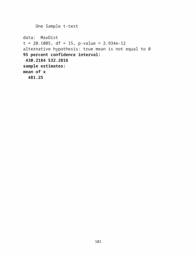
The ANOVA Hypotheses:

H0: ___________________ versus Ha: _____________________________________________

Notice this alternative does not require all the population means be different from each other.

One possible Ha picture

Question: What call a technique for testing the equality of the means “analysis of VARIANCE”?

Answer: We are going to compare two estimators of the common population variance, σ2

.

MS Groups (Mean Square between the Groups):

MSE (Mean Square Within or due to Error):

These two estimates are used to form the F statistic:

F= Variation among sample meansNatural variation within groups =

MS GroupsMSE .

If this F ratio is too ______ we would reject the null hypothesis.

182

The Logic behind the ANOVA F-Test

Look at the plots below. For each Scenario, we have plotted data obtained by taking independent random samples of size 10 from three populations.

For Scenarios A and B, the three populations each had a normal distribution and the population means were 60, 65, and 70, respectively. So the population means are indeed not all equal.

In Scenario A, the population standard deviations were all equal to 1.5. In Scenario B, the population standard deviations were all equal to 3. So in each case the assumption that the populations have equal standard deviations is met.

Scenario A

Scenario B

All images

Which of the above two scenarios do you think would provide more evidence that at least one of the population means is different from the others? Scenario A or Scenario B?

Samples from 3 populations whose means are different.

Variability within each population is small.

Difference between sample means more readily seen.

F statistic somewhat big.

Samples from 3 populations whose means are different.

Variability within each population is larger.

Difference between sample means not readily seen.

F statistic smaller.

183

Below is a final set of plots for three independent random samples of size 10 each taken from a population with a normal model with a population mean of 65 and population standard deviation of 1.5. So in Scenario C, the population means are indeed all equal––that is, the null hypothesis tested in one-way ANOVA is true. Notice that, although the population means were all equal, there is still some of variation between the sample means.

Also in Scenario C there is still some natural variation within the samples, making the slight variation between the sample means hardly noticeable. The data in Scenario C do not provide evidence that the population means are different. Scenario C

The F-statistic will be sensitive to differences between the sample means. The larger the variation between the sample means, the larger the value of the F-statistic and larger values of the F-statistic provide more support for rejecting the null hypothesis. The variation between the sample means was greatest for Scenarios A and B compared to Scenario C. The natural variation within the samples was greatest for Scenario B compared to Scenarios A and C. The F-statistic is the ratio of these two measures of variation:

F= Variation among sample meansNatural variation within groups

So which scenario would you expect to result in the largest value of the F-statistic? Provided below are the values of the F-statistic for the test of equality of the population means.

Scenario Value of F Statistic p-valueA (Ha is true) F = 80.4 0.0000B (Ha is true) F = 16.4 0.01C (H0 is true) F = 0.17 0.84

Note the value of the F-statistic is smallest and the p-value the largest when the null hypothesis is true (Scenario C). For Scenarios A and B, the population means are different, but the smaller population standard deviation in Scenario A accentuates the differences by producing a larger F-ratio and an extremely small p-value. A larger F-statistic value (and thus smaller p-value) corresponds to more evidence that the population means are not all equal.

Samples from 3 populations whose means are all equal.

Still some variability within each population.

Very little differences between the sample means.

F statistic very small.

184

Computing the F Test StatisticWe will see how to get MS Groups and MSE and perform the F test. These two mean squares will be a sum of squares (SS) divided by a corresponding degrees of freedom (DF).

The data can be generically represented below, where X ij= jth observation from the ith

population. However we really don’t have to worry too much about these subscripts, as we will go through the steps using words!

Data from Population1 Data from Population 2 … Data from Population kX11 X21 X k1X12 X22 X k2

⋮ ⋮ ⋮X1 n1

X2 n2X knk

The details leading to the F statistic are presented in six steps, ending with an ANOVA table.

Step 1: Calculate the mean and variance for each sample: x i , si2

Step 2: Calculate the overall sample mean

(using all N=n1+n2+.. .+nk observations): x

Step 3: Calculate the sum of squares between groups:

SS Groups=∑groups

ni ( x i− x )2

Step 4: Calculate the sum of squares within groups (due to error):

SSE=∑groups (n i−1 ) si2

Step 5: OPTIONAL: Calculate the total sum of squares:

SS Total=∑values (x ij− x )2

Step 6: Fill in the ANOVA table:

Source DF Sum of Squares Mean Square F

Groups k-1 SS Groups

185

Error (Within) N-k SSE

Total N-1 SS Total

If H0 is true, then the F statistic, F=MS Groups

MSE , has an F(k – 1, N – k) distribution. Below are a few pictures of some F distributions.

From Utts, Jessica M. and Robert F. Heckard. Mind on Statistics, Fourth Edition. 2012. Used with permission.

Table A.4 provides percentiles of an F distribution. However, standard computer output also provides the exact p-value and completed ANOVA table. We will rely on R output to provide the p-value, but you should know how the ANOVA table is constructed and be able to sketch a picture of the p-value for an F-test.

Stat 250 Formula Card Summary of ANOVA

Try It! Comparing 3 DrugsWe wish to compare three drugs for treating some disease. A quantitative response (time to cure in days) is measured such that a smaller value indicates a more favorable response.

A total of N=19 patients are randomly assigned to one of the three drug (treatment) groups. The data are provided below:

Drug 1 Drug 2 Drug 37.3 7.1 5.88.2 10.6 6.5

10.1 11.2 8.86.0 9.0 4.99.5 8.5 7.9

10.9 8.5

186

7.8 5.2

187

Recall the assumptions for performing an F-test. Think about how you would check them. Each sample is a ... random sample The k random samples are ... independent For each of population the model for the response is... a normal distribution The k population variances are .... equal.

State the hypotheses to be tested:

H0: _____________________ Ha:___________________________________________

Note: We would use a computer or calculator to work at least the basic summaries in steps 1 and 2, and likely to create the entire ANOVA table for us. Let’s be sure we understand where the values are coming from and how to interpret the final results.

Step 1: Calculate the mean and variance for each sample:

x1= s12=

x2= s22=

x3= s32=

Step 2: Calculate the overall sample mean (based on all N=n1+n2+.. .+nk observations):

x=

Step 3: Calculate the sum of squares between groups:

SS Groups=∑groupsni ( x i− x )2

Step 4: Calculate the sum of squares within groups (due to error):

SSE=∑groups (n i−1 ) si2

188

Step 5: OPTIONAL: Calculate the total sum of squares: No Thank You!

Step 6: Fill in the ANOVA table:

Source Sum of Squares DF Mean Square FGroups

Error (Within)

Total

Here are the results from R:

Df Sum Sq Mean Sq F value Pr(>F) DrugID 2 21.98 10.991 4.188 0.0345 *Residuals 16 41.99 2.624 ---Signif. codes: 0 '***' 0.001 '**' 0.01 '*' 0.05 '.' 0.1 ' ' 1

One of the assumptions in ANOVA is that the population standard deviations are all equal. Using the data, give an estimate of this common population standard deviation.

Give the observed test statistic value.

What is the distribution of the test statistic if the three drugs are equally effective in terms of the mean response?

What is the corresponding p-value for assessing if the three drugs are equally effective in terms of the mean response?

At the 5% level, what is your conclusion?

189

We Rejected H0 in ANOVA: What is next? Multiple ComparisonsThe term multiple comparisons is used when two or more comparisons are made to examine the specific pattern of differences among means. The most commonly analyzed set of multiple comparisons is the set of all pairwise comparisons among population means. In our previous Drug example, the possible pairwise comparisons are: Drug 1 with Drug 2, Drug 1 with Drug 3, and Drug 2 with Drug 3. To compare the pair of means we could …

Compute a confidence interval for the difference between the two population means and see if 0 falls in the interval or not.

Perform a test of hypotheses to assess if the two population means differ significantly.

When many statistical tests are done there is an increased risk of making at least one type I error (erroneously rejecting a null hypothesis). Consequently, several procedures have been developed to control the overall family type I error rate or the overall family confidence level when inferences for a set (family) of multiple comparisons are done.

Tukey’s procedure is one such procedure for the family of pairwise comparisons. If the family error rate is not a concern, Fisher’s procedure is used.

Try It! Comparing 3 DrugsIn the comparison of the three drugs, we rejected the null hypothesis at the 5% significance level. We follow with a multiple comparison procedure to determine which group means are significantly different from each other.

R gives family-wise confidence interval comparisons using Tukey's method and a family confidence level of 95%.

95% family-wise confidence level

Linear Hypotheses: Estimate lwr upr II - I == 0 1.0800 -1.3670 3.5270III - I == 0 -1.4200 -3.8670 1.0270III - II == 0 -2.5000 -4.7338 -0.2662

I II III "ab" "b" "a"

a. Use the above output to report about the three pairwise comparisons:Does the confidence interval for comparing Drug I and II contain 0? __________ Does the confidence interval for comparing Drug I and III contain 0? __________ Does the confidence interval for comparing Drug II and III contain 0? __________

b. State your conclusions regarding the differences between the mean response for the three drug groups based on the Tukey family-wise comparison method.

We can conclude that the population mean responses differ for …

190

but do not differ for …Individual Confidence Intervals for the Population Means Sometimes it is helpful to examine a confidence interval for the mean for each population. Since in ANOVA we assume the population standard deviations are all equal, the estimate of

that common population standard deviation sp=√MSE is used in forming the individual confidence intervals. The degrees of freedom used to find the t* multiplier will be those associated with the estimated standard deviation, namely N – k. The formula for the individual confidence intervals is provided below.

Try It! Comparing 3 DrugsWe were comparing k = 3 groups based on a total of N = 19 observations. The pooled standard deviation for the comparison of the three drugs data set is sp = 1.62. The sample means and sample sizes were:

Drug 1: Sample mean = 8.22 Sample size = 5Drug 2: Sample mean = 9.30 Sample size = 7Drug 3: Sample mean = 6.80 Sample size = 7

The degrees of freedom for the t* multiplier is N – k = _________________.

From the table of t* multipliers (Table A.2) with confidence level = 0.95

and the above degrees of freedom we have t* = ____________________

Drug 3 was descriptively the best. Compute a 95% confidence interval for the population mean time to cure for all subjects taking Drug 3.

191

Try It! Memory ExperimentIn a memory experiment, three groups of subjects were given a list of words to try to remember. The length of the list for the first group was 10 words (short list), whereas for the second group it was 20 words (medium list) and for the third group 40 words (long list). The percentage of words recalled for each subject was recorded. The sample mean percentage of words recalled was 68.3% for the short list, 48% for the medium list, and 39.2%for the long list. A one-way ANOVA was used to assess whether the length of the list had a significant effect on the percentage of words recalled.

df SS Mean Square F Sig.List Length 2 2668.8 .0003

Residuals 84.6

Total 16 3852.9a. Some values in the ANOVA table are missing. Complete the above table.b. State the null and alternative hypotheses that the above F statistic is testing.

H0: ____________________ vs. Ha:__________________________________c. Suppose the necessary assumptions hold. Using a 5% significance level, does it appear that

the average percentage of words recalled is the same for the three different lengths of lists? Explain.

d. Family-wise comparisons were performed using Tukey’s method.

95% family-wise confidence level

Linear Hypotheses: Estimate lwr upr medium - short == 0 -20.33 -39.61 -1.06long - short == 0 -29.17 -47.54 -10.79long - medium == 0 -8.83 -28.11 10.44

short medium long "a" "a"

Use the results and circle the pairs that are significantly different at a 5% level. short versus medium short versus long medium versus long

e. Give a 99% confidence interval for the population mean percentage of words recalled for the long list group. Recall that the sample mean based on the 6 subjects in the long list group was 39.2 percent.

192

What if some conditions do not hold?You probably won’t be surprised to learn that the necessary conditions for using an analysis of variance F-test don’t hold for all data sets. There are methods that can be used when one or both of the assumptions about equal population standard deviations and normal distributions are violated.

When the observed data are skewed, or when extreme outliers are present, it usually is better to analyze the median rather than the mean. One test for comparing medians is the Kruskal-Wallis Test. It is based on a comparison of the relative rankings (sizes) of the data in the observed samples, and for this reason is called a rank test. The term nonparametric test also is used to describe this test because there are no assumptions made about a specific distribution for the population of measurements. Another nonparametric test used to compare population medians is Mood’s Median Test.

Two-Way ANOVASo far we have focused on the one-way ANOVA procedure. The "one-way" referred to having only one explanatory variable (or factor) and one quantitative response variable.

Two-way ANOVA examines the effect of two explanatory variables (or factors) on the mean response. The researcher is interested in the individual effect of each explanatory variable on the mean response and also in the combined effect of the two explanatory variables on the mean response. The individual effect of each factor on the response is called a main effect. If one of the factors does not have an effect on the response, we say there is no main effect due to that factor.

Besides assessing the main effects of each factor on the response, an interesting feature in two-way analyses is the possibility of interaction between the two factors. We say there is interaction between two factors if the effect of one factor on the mean response depends on the specific level of the other factor. The interpretation of the factor main effects can be more difficult when interaction is present.

Additional NotesA place to … jot down questions you may have and ask during office hours, take a few extra notes, write out an extra problem or summary completed in lecture, create your own summary about these

concepts.

193

Stat 250 Gunderson Lecture Notes11: Regression Analysis

The invalid assumption that correlation implies cause is probably among the two or three most serious and common errors of human reasoning.

--Stephen Jay Gould, The Mismeasure of Man

Describing and assessing the significance of relationships between variables is very important in research. We will first learn how to do this in the case when the two variables are quantitative. Quantitative variables have numerical values that can be ordered according to those values.

Main ideaWe wish to study the relationship between two quantitative variables.

Generally one variable is the ________________________ variable, denoted by y. This variable measures the outcome of the study

and is also called the ________________________ variable.

The other variable is the ________________________ variable, denoted by x. It is the variable that is thought to explain the changes we see in the response variable.

The explanatory variable is also called the ________________ variable.

The first step in examining the relationship is to use a graph - a scatterplot - to display the relationship. We will look for an overall pattern and see if there are any departures from this overall pattern.

If a linear relationship appears to be reasonable from the scatterplot, we will take the next step of finding a model (an equation of a line) to summarize the relationship. The resulting equation may be used for predicting the response for various values of the explanatory variable. If certain assumptions hold, we can assess the significance of the linear relationship and make some confidence intervals for our estimations and predictions.

Let's begin with an example that we will carry throughout our discussions.

194

Graphing the Relationship: Restaurant Bill vs TipHow well does the size of a restaurant bill predict the tip the server receives? Below are the bills and tips from six different restaurant visits in dollars.

Bill 41 98 25 85 50 73Tip 8 17 4 12 5 14

Response (dependent) variable y = ________ .

Explanatory (independent) variable x = _________ .

Step 1: Examine the data graphically with a scatterplot.Add the points to the scatterplot below:

Interpret the scatterplot in terms of ... overall form (is the average pattern look like a straight line or is it curved?) direction of association (positive or negative) strength of association (how much do the points vary around the average pattern?) any deviations from the overall form?

195

Describing a Linear Relationship with a Regression LineRegression analysis is the area of statistics used to examine the relationship between a quantitative response variable and one or more explanatory variables. A key element is the estimation of an equation that describes how, on average, the response variable is related to the explanatory variables. A regression equation can also be used to make predictions.

The simplest kind of relationship between two variables is a straight line, the analysis in this case is called linear regression.

Regression Line for Bill vs. Tip Remember the equation of a line? In statistics we denote the regression line for a sample as:where:

y

b0

b1

Goal: To find a line that is “close” to the data points - find the “best fitting” line.

How? What do we mean by best? One measure of how good a line fits is to look at the “observed errors” in prediction.

Observed errors = _____________________

are called ____________________

So we want to choose the line for which the sum of squares of the observed errors (the sum of squared residuals) is the least.

The line that does this is called:_______________________________________

196

The equations for the estimated slope and intercept are given by:

b1=

b0=

The least squares regression line (estimated regression function) is: y= μ y( x )=b0+b1 x

To find this estimated regression line for our exam data by hand, it is easier if we set up a calculation table. By filling in this table and computing the column totals, we will have all of the main summaries needed to perform a complete linear regression analysis. Note that here we have n = 6 observations. The first five rows have been completed for you. In general, use R or a calculator to help with the graphing and numerical computations!

x = bill y = tip x− x ( x− x )2 ( x− x ) y y− y ( y− y )2

41 8 41–62 = -21 (-21)2 = 441 (-21)(8)= -168 8–10 = -2 (-2)2 = 4

98 17 98–62 = 36 (36)2 = 1296 (36)(17)= 612 17–10 = 7 (7)2 = 49

25 4 25–62 = -37 (-37)2 = 1369 (-37)(4)= -148 4–10 = -6 (-6)2 = 36

85 12 85–62 = 23 (23)2 = 529 (23)(12)= 276 12–10 = 2 (2)2 = 4

50 5 50–62 = -12 (-12)2 = 144 (-12)(5)= -60 5–10 = -5 (-5)2 = 25

73 14

372 60

x= 3726

=62 ӯ=606

=10

Slope Estimate:

y-intercept Estimate:

Estimated Regression Line:

197

Predict the tip for a dinner guest who had a $50 bill.

Note: The 5th dinner guest in sample had a bill of $50 and the observed tip was $5.

Find the residual for the 5th observation.

Notation for a residual =e5= y5− y5=

The residuals …

You found the residual for one observation. You could compute the residual for each observation. The following table shows each residual.

x = bill y = tippredicted values

y=−0.5877+0.17077( x)residualse= y− y

Squared residuals

(e )2=( y− y )241 8 6.41 1.59 2.5298 17 16.15 0.85 0.7225 4 3.68 0.32 0.1085 12 13.93 -1.93 3.7350 5 7.95 -2.95 8.7073 14 11.88 2.12 4.49

-- -- --

SSE = sum of squared errors (or residuals)

198

Measuring Strength and Direction of a Linear Relationship with Correlation The correlation coefficient r is a measure of strength of the linear relationship between y and x.

Properties about the Correlation Coefficient r

1. r ranges from ...

2. Sign of r indicates ...

3. Magnitude of r indicates ...

A “strong” r is discipline specificr = 0.8 might be an important (or strong) correlation in engineeringr = 0.6 might be a strong correlation in psychology or medical research

4. r ONLY measures the strength of the ______ relationship.

Some pictures:

The formula for the correlation:(but we will get it from computer output or from r2)

Tips Example:

r = ____________

Interpretation:

199

The square of the correlation r2

The squared correlation coefficient r2

always has a value between ___________ and is sometimes presented as a percent. It can be shown that the square of the correlation is related to the sums of squares that arise in regression.

The responses (the amount of tip) in data set are not all the same - they do vary. We would

measure the total variation in these responses as SSTO=∑ ( y− y )2 (last column total in calculation table said we would use later).

Part of the reason why the amount of tip varies is because there is a linear relationship between amount of tip and amount of bill, and the study included different amounts of bill.

When we found the least squares regression line, there was still some small variation remaining of the responses from the line. This amount of variation that is not accounted for by the linear relationship is called the SSE.

The amount of variation that is accounted for by the linear relationship is called the sum of squares due to the model (or regression), denoted by SSM (or sometimes as SSR).

So we have: SSTO = ____________________________________It can be shown that

r2=

= the proportion of total variability in the responses that can be explained by the linear relationship with the explanatory variable x .

200

Note: The value of r2

and these sums of squares are summarized in an ANOVA table that is standard output from computer packages when doing regression.Measuring Strength and Direction for Exam 2 vs Final

From our first calculation table we have:

SSTO = ______________________________________

From our residual calculation table we have:

SSE = _____________________________________

So the squared correlation coefficient for our exam scores regression is:

r2= SSTO−SSESSTO =

Interpretation:We accounted for ___ % of the variation in _______________________

by the linear regression on .

The correlation coefficient is r = ___________________

A few more general notes:

Nonlinear relationships

Detecting Outliers and their influence on regression results.

Dangers of Extrapolation (predicting outside the range of your data)

Dangers of combining groups inappropriately (Simpson’s Paradox)

Correlation does not prove causation

201

R Regression Analysis for Bill vs Tips

Let’s look at the R output for our Bill and Tip data.We will see that much of the computations are done for us.

Call:lm(formula = Tip ~ Bill, data = Tips)

Residuals: 1 2 3 4 5 6 1.5862 0.8523 0.3185 -1.9277 -2.9508 2.1215

Coefficients: Estimate Std. Error t value Pr(>|t|) (Intercept) -0.58769 2.41633 -0.243 0.81980 Bill 0.17077 0.03604 4.738 0.00905 **---Signif. codes: 0 '***' 0.001 '**' 0.01 '*' 0.05 '.' 0.1 ' ' 1

Residual standard error: 2.251 on 4 degrees of freedomMultiple R-squared: 0.8487, Adjusted R-squared: 0.8109 F-statistic: 22.45 on 1 and 4 DF, p-value: 0.009052

Correlation “Matrix”

Bill TipBill 1.0000000 0.9212755Tip 0.9212755 1.0000000

ANOVA Table

Response: Tip Df Sum Sq Mean Sq F value Pr(>F) Bill 1 113.732 113.732 22.446 0.009052 **Residuals 4 20.268 5.067

202

---Signif. codes: 0 '***' 0.001 '**' 0.01 '*' 0.05 '.' 0.1 ' ' 1

203

Inference in Linear Regression AnalysisThe material covered so far focuses on using the data for a sample to graph and describe the relationship. The slope and intercept values we have computed are statistics, they are estimates of the underlying true relationship for the larger population.

Next we turn to making inferences about the relationship for the larger population. Here is a nice summary to help us distinguish between the regression line for the sample and the regression line for the population.

Regression Line for the Sample

Regression Line for the Population

All images

204

To do formal inference, we think of our b0 and b1 as estimates of the unknown parameters 0

and 1 . Below we have the somewhat statistical way of expressing the underlying model that produces our data:

Linear Model: the response y = [0 + 1(x)] + = [Population relationship] + Randomness

This statistical model for simple linear regression assumes that for each value of x the observed values of the response (the population of y values) is normally distributed, varying around some true mean (that may depend on x in a linear way) and a standard deviation that does not depend on x. This true mean is sometimes expressed as E(Y) = 0 + 1(x). And the components and assumptions regarding this statistical model are show visually below.

The represents the true error term. These would be the deviations of a particular value of the response y from the true regression line. As these are the deviations from the mean, then these error terms should have a normal distribution with mean 0 and constant standard deviation .

Now, we cannot observe theseε ’s. However we will be able to use the estimated (observable) errors, namely the residuals, to come up with an estimate of the standard deviation and to check the conditions about the true errors.

True regressionline

x

205

So what have we done, and where are we going? 1. Estimate the regression line based on some data. DONE!2. Measure the strength of the linear relationship with the correlation. DONE!3. Use the estimated equation for predictions. DONE!4. Assess if the linear relationship is statistically significant. 5. Provide interval estimates (confidence intervals) for our predictions.6. Understand and check the assumptions of our model.

We have already discussed the descriptive goals of 1, 2, and 3. For the inferential goals of 4 and 5, we will need an estimate of the unknown standard deviation in regression

Estimating the Standard Deviation for RegressionThe standard deviation for regression can be thought of as measuring the average size of the residuals. A relatively small standard deviation from the regression line indicates that individual data points generally fall close to the line, so predictions based on the line will be close to the actual values.

It seems reasonable that our estimate of this average size of the residuals be based on the residuals using the sum of squared residuals and dividing by appropriate degrees of freedom. Our estimate of is given by:

s =

Note: Why n – 2?

Estimating the Standard Deviation: Bill vs TipBelow are the portions of the R regression output that we could use to obtain the estimate of for our regression analysis.

From Summary:

Residual standard error: 2.251 on 4 degrees of freedomMultiple R-squared: 0.8487, Adjusted R-squared: 0.8109 F-statistic: 22.45 on 1 and 4 DF, p-value: 0.009052

Or from ANOVA:

Response: Tip Df Sum Sq Mean Sq F value Pr(>F) Bill 1 113.732 113.732 22.446 0.009052 **Residuals 4 20.268 5.067

206

Significant Linear Relationship?

Consider the following hypotheses: H0 : β1=0 versus Ha : β1≠0What happens if the null hypothesis is true?

There are a number of ways to test this hypothesis. One way is through a t-test statistic (think about why it is a t and not a z test). The general form for a t test statistic is:

t= sample statistic - null valuestandard error of the sample statistic

We have our sample estimate for β1 , it is b1 . And we have the null value of 0. So we need the

standard error for b1 . We could “derive” it, using the idea of sampling distributions (think about

the population of all possible b1 values if we were to repeat this procedure over and over many times). Here is the result:

t-test for the population slope β1

To test H0 : β1=0 we would use t=

b1−0s .e .( b1 )

where SE(b1 )=

s

√∑ ( x− x )2 and the degrees of freedom for the t-distribution are n – 2.

This t-statistic could be modified to test a variety of hypotheses about the population slope (different null values and various directions of extreme).

Try It! Significant Relationship between Bill and Tip?Is there a significant (non-zero) linear relationship between the total cost of a restaurant bill and the tip that is left? (is the bill a useful linear predictor for the tip?)

That is, test H0 : β1=0 versus Ha : β1≠0 using a 5% level of significance.

207

Think about it: Based on the results of the previous t-test conducted at the 5% significance level, do you think a

95% confidence interval for the true slope β1 would contain the value of 0?

Confidence Interval for the population slope β1

b1±t∗[SE (b1) ] where df = n – 2 for the t∗¿ ¿ value

Compute the interval and check your answer.

Could you interpret the 95% confidence level here?

Inference about the Population Slope using RBelow are the portions of the R regression output that we could use to perform the t-test and

obtain the confidence interval for the population slope β1 .

Coefficients: Estimate Std. Error t value Pr(>|t|) (Intercept) -0.58769 2.41633 -0.243 0.81980 Bill 0.17077 0.03604 4.738 0.00905 **

Note: There is a third way to test H0 : β1=0 versus Ha : β1≠0 . It involves another F-test from an ANOVA for regression.

Response: Tip Df Sum Sq Mean Sq F value Pr(>F) Bill 1 113.732 113.732 22.446 0.009052 **Residuals 4 20.268 5.067

208

Predicting for Individuals versus Estimating the MeanConsider the relationship between the bill and tip …

Least squares regression line (or estimated regression function):

y=

We also have: s=

How would you predict the tip for Barb who had a $50 restaurant bill?

How would you estimate the mean tip for all customers who had a $50 restaurant bill?

So our estimate for predicting a future observation and for estimating the mean response are found using the same least squares regression equation. What about their standard errors? (We would need the standard errors to be able to produce an interval estimate.)

Idea: Consider a population of individuals and a population of means:

What is the standard deviation for a population of individuals?

What is the standard deviation for a population of means?Which standard deviation is larger?

So a prediction interval for an individual response will be

(wider or narrower) than a confidence interval for a mean response.

209

Here are the (somewhat messy) formulas:

Confidence interval for a mean response:

y± t¿ s .e .( fit )

where

s .e .( fit )=s √ 1n+

( x− x )2

∑ ( xi− x )2 df = n – 2

Prediction interval for an individual response:

y±t¿ s .e .(pred )

where s .e .(pred )=√s2+( s .e .( fit ))2 df = n – 2

Try It! Bill vs TipConstruct a 95% confidence interval for the mean tip given for all customers who had a $50 bill

(x). Recall: n = 6, x=62, ∑ (x− x )2=SXX=940 3900, y= -0.58 +0.17(x), and s = 2.251.

Construct a 95% prediction interval for the tip from an individual customer who had a $50 bill (x).

210

Checking Assumptions in RegressionLet’s recall the statistical way of expressing the underlying model that produces our data:

Linear Model: the response y = [0 + 1(x)] + = [Population relationship] + Randomness

where the ‘s, the true error terms should be normally distributed with mean 0 and constant standard deviation , and this randomness is independent from one case to another.

Thus there are four essential technical assumptions required for inference in linear regression:

(1) Relationship is in fact linear. (2) Errors should be normally distributed.(3) Errors should have constant variance.(4) Errors should not display obvious ‘patterns’.

Now, we cannot observe theseε ’s. However we will be able to use the estimated (observable) errors, namely the residuals, to come up with an estimate of the standard deviation and to check the conditions about the true errors.

So how can we check these assumptions with our data and estimated model?

(1) Relationship is in fact linear.

(2) Errors should be normally distributed.

(3) Errors should have constant variance. If we see …(4) Errors should not display obvious ‘patterns’.

Now, if we saw …

211

Let's turn to one last full regression problem that includes checking assumptions.

Relationship between height and foot length for College Men

The heights (in inches) and foot lengths (in centimeters) of 32 college men were used to develop a model for the relationship between height and foot length. The scatterplot and R regression output are provided.

mean sd nfoot 27.78125 1.549701 32height 71.68750 3.057909 32

Call:lm(formula = foot ~ height, data = heightfoot)

Residuals: Min 1Q Median 3Q Max -1.74925 -0.81825 0.07875 0.58075 2.25075

Coefficients: Estimate Std. Error t value Pr(>|t|) (Intercept) 0.25313 4.33232 0.058 0.954 height 0.38400 0.06038 6.360 5.12e-07 ***---Signif. codes: 0 '***' 0.001 '**' 0.01 '*' 0.05 '.' 0.1 ' ' 1

Residual standard error: 1.028 on 30 degrees of freedomMultiple R-squared: 0.5741, Adjusted R-squared: 0.5599 F-statistic: 40.45 on 1 and 30 DF, p-value: 5.124e-07

Correlation Matrix

foot heightfoot 1.0000000 0.7577219height 0.7577219 1.0000000

Analysis of Variance Table

Response: foot

212

Df Sum Sq Mean Sq F value Pr(>F) height 1 42.744 42.744 40.446 5.124e-07 ***Residuals 30 31.705 1.057

Also note that: SXX = ∑ (x− x )2 = 289.87

213

a. How much would you expect foot length to increase for each 1-inch increase in height? Include the units.

b. What is the correlation between height and foot length?

c. Give the equation of the least squares regression line for predicting foot length from height.

d. Suppose Max is 70 inches tall and has a foot length of 28.5 centimeters. Based on the least squares regression line, what is the value of the prediction error (residual) for Max? Show all work.

e. Use a 1% significance level to assess if there is a significant positive linear relationship

between height and foot length. State the hypotheses to be tested, the observed value of the test statistic, the corresponding p-value, and your decision.

Hypotheses: H0:____________________Ha:________________________

Test Statistic Value: _______________ p-value: ___________________

Decision: (circle) Fail to reject H0 Reject H0

Conclusion:

214

f. Calculate a 95% confidence interval for the average foot length for all college men who are 70 inches tall. (Just clearly plug in all numerical values.)

g. Consider the residuals vs fitted plot shown.

Does this plot support the conclusion that the linear regression model is appropriate?

Yes No

Explain:

215

RegressionLinear Regression Model

Population Version:Mean: xYExY 10)(

Individual: iii xy 10

where i is ),0( N

Sample Version:

Mean: xbby 10ˆ

Individual: iii exbby 10

Standard Error of the Sample Slope

21 )(s.e.

xx

sSsbXX

Confidence Interval for 1

)(s.e. 1*

1 btb df = n – 2

t-Test for 1 To test 0: 10 H )(s.e.0

1

1

bb

t

df = n – 2

or MSEMSREGF

df = 1, n – 2Parameter Estimators

221xx

yxx

xx

yyxx

SS

bXX

XY

xbyb 10

Confidence Interval for the Mean Responses.e.(fit)ˆ *ty df = n – 2

where XXSxx

ns

2)(1)fit(s.e.

Residualsyye ˆ = observed y – predicted y

Prediction Interval for an Individual Responses.e.(pred)ˆ *ty df = n – 2

where 22 )fit(s.e.s.e.(pred) s

Correlation and its square

YYXX

XY

SS

Sr

SSTOSSREG

SSTOSSESSTOr

2

where 2 yySSSTO YY

Standard Error of the Sample Intercept

XXSx

nsb

2

01)(s.e.

Confidence Interval for 0

)(s.e. 0*

0 btb df = n – 2

Estimate of

2

nSSEMSEs

where 22

ˆ eyySSE

t-Test for 0 To test 0: 00 H

)(s.e.0

0

0

bb

t

df = n – 2

216

Additional NotesA place to … jot down questions you may have and ask during office hours, take a few extra notes, write out an extra problem or summary completed in lecture, create your own summary about these

concepts.

217

Stat 250 Gunderson Lecture NotesRelationships between Categorical Variables

12: Chi-Square Analysis

Inference for Categorical Variables

Having now covered a lot of inference techniques for quantitative responses, we return to analyzing categorical data, that is, analyzing count data. The three main tests described in the text that we will cover are:

1. Goodness of Fit Test: this test is for assessing if a particular discrete model is a good fitting model for a discrete characteristic, based on a random sample from the population.E.g. Has the model for the method of transportation (drive, bike, walk, other)

used by students to get the class changed from that for 5 years ago?

2. Test of Homogeneity: this test is for assessing if two or more populations are homogeneous (alike) with respect to the distribution of some discrete (categorical) variable.E.g. Is the distribution of opinion on legal gambling the same for adult males

versus adult females?

3. Test of Independence: this test helps us to assess if two discrete (categorical) variables are independent for a population, or if there is an association between the two variables.E.g. Is there an association between satisfaction with the quality of public schools

(not satisfied, somewhat satisfied, very satisfied) and political party (Republican, Democrat, etc.)

The first test is the one-sample test for count data. The other two tests (homogeneity and independence) are actually the same test. Although the hypotheses are stated differently and the underlying assumptions about how the data is gathered are different, the steps for doing the two tests are exactly the same.

All three tests are based on an X2

test statistic that, if the corresponding H0 is true and the assumptions hold, follows a chi-square distribution with some degrees of freedom, written χ2 (df ) . So our first discussion is to learn about the chi-square distribution - what the distribution looks like, some facts, how to use Table A.5 to find various percentiles.

218

The Chi-Square DistributionGeneral Shape:If we have a chi-square distribution with df = degrees of freedom, then the ...

Mean is equal to

Variance is equal to

Standard deviation

is equal to

These facts will serve as a useful frame of reference for making decision.

All imagesTable A.5 provides some upper-tail percentiles for chi-square distributions.

From Utts, Jessica M. and Robert F. Heckard. Mind on Statistics, Fourth Edition. 2012. Used with permission.

Try It! Consider the χ2 (4 ) distribution.

a. What is the mean for this distribution? __________

b. What is the median for this distribution? __________

c. How likely would it be to get a value of 4 or even larger?

d. How likely would it be to get a value of 10.3 or even larger?

219

The BIG IDEA The data consists of observed counts. We compute expected counts under the H0 - these counts are what we would expect

(on average) if the corresponding H0 were true. Compare the observed and expected counts using the X

2 test statistic. The statistic will

be a measure of how close the observed counts are to the expected counts under H0. If this distance is large, we have support for the alternative Ha.

With this in mind, we turn to our first chi-square test of goodness of fit. We will derive the methodology for the test through an example. An overall summary of the test will be presented at the end.

Test of Goodness of Fit: Helps us assess if a particular discrete model is a good fitting model for a discrete characteristic, based on a random sample from the population.

Goodness of Fit Test

Scenario: We have one population of interest, say all cars exiting a toll road that has four booths at the exit.

Question: Are the four booths used equally often?

Data: One random sample of 100 cars, we record one variable X, which booth was used (1, 2, 3, 4). The table below summarizes the data in terms of the observed counts.

Booth 1 Booth 2 Booth 3 Booth 4Observed # cars 26 20 28 26

Note: This is only a one-way frequency table, not a two-way table as will be in the homogeneity and independence tests. We use the notation k = the number of categories or cells, here k=4 .

The null hypothesis:

Let pi = (population) proportion of cars using booth i

H0: p1 = , p2 = , p3 = , p4 = .

Ha: ______________________________________________________________

The null hypothesis specifies a particular discrete model (mass function) by listing the proportions (or probabilities) for each of the k outcome categories.

220

The one-way table provides the OBSERVED counts. Our next step is to compute the EXPECTED counts, under the assumption that H0 is true.

How to find the expected counts?There were 100 cars in the sample and 4 booths.

If the booths are used equally often, H0 is true, then we would expect

... cars to use Booth #1

... cars to use Booth #2

... cars to use Booth #3

... cars to use Booth #4

Expected Counts =E i=npiEnter these expected counts in the parentheses in the table below.

Observed Counts (Expected Counts)}Booth 1 Booth 2 Booth 3 Booth 4

Number of cars 26 ( ) 20 ( ) 28 ( ) 26 ( ) The X

2 test statistic

Next we need our test statistic, our measure of how close the observed counts are to what we expect under the null hypothesis.

X2=

Do you think a value of X2= is large enough to reject H0?

Let's find the p-value, the probability of getting an X2

test statistic value as large or larger than the one we observed, assuming H0 is true. To do this we need to know the distribution of the X2

test statistic under the null hypothesis.

If H0 is true, then X2

has the χ2

distribution with degrees of freedom = .

221

222

Find the p-value for our tollbooth example:

Observed X2

test statistic value = df = .

Are the results statistically significant at the 5% significance level?Conclusion at a 5% level: It appears that ....

Aside: Using our frame of reference for chi-square distributions.Recall that if we have a chi-square distribution with df = degrees of freedom, then the mean is

equal to df , and the standard deviation is equal to √2(df )

So, if H0 were true, we would expect the X2

test statistic to be about give or take about .

Since we reject H0 for large values of X2

, and we only observed a value of , even less than expected under H0, we certainly do not have enough evidence to reject H0.

Goodness of Fit Test Summary

Assume: We have 1 random sample of size n . We measure one discrete response X that has k possible outcomes

Test: H0: A specified discrete model for X p1= p10 , p2=p20 , …, pk=pk0

Ha: The probabilities are not as specified in the null hypothesis.

Test Statistic:X2=∑ (observed - expected )2

expected

where expected =E i=npi0

If H0 is true, then X2

has a χ2

distribution with (k−1) degrees of freedom, where k is the number of categories. The necessary conditions are: at least 80% of the expected counts are greater than 5 and none are less than 1. Be aware of the sample size (pg 656).

223

224

Try It! Crossbreeding PeasFor a genetics experiment in the cross breeding of peas, Mendel obtained the following data in a sample from the second generation of seeds resulting from crossing yellow round peas and green wrinkled peas.

Yellow Round Yellow Wrinkled Green Round Green Wrinkled315 101 108 32

Do these data support the theory that these four types should occur with probabilities 9/16, 3/16, 3/16, and 1/16 respectively? Use = 0.01.

Try It! Desired Vacation PlaceThe AAA travel agency would like to assess if the distribution of desired vacation place has changed from the model of 3 years ago. A random sample of 928 adults were polled by the polling company Ipsos during this past mid-May. One question asked was “Name the one place you would want to go for vacation if you had the time and the money.” The table displays the model for the distribution of desired vacation place 3 years ago and the observed results based on the recent poll.

1 = Hawaii 2 = Europe 3 = Caribbean 4 = Other TotalsModel

3 years ago 10% 40% 20% 30% 100%

Obs Counts from poll 124 390 125 289 928

a. Give the null hypothesis to test if there has been a significant change in the distribution of desired vacation place from 3 years ago.

b. The observed test statistic is ~ 31 and the p-value is less than 0.001. Interpret this p-value in terms of repeated random samples of 928 adults.

225

Test of Homogeneity: Helps us to assess if the distribution for one discrete (categorical) variable is the same for two or more populations.

Test of Homogeneity

Scenario: We have 2 populations of interest; preschool boys and preschool girls.Question: Is Ice Cream Preference the same for boys and girls?

Data: 1 random sample of 75 preschool boys, 1 random sample of 75 preschool girls; the two random samples are independent.

The table below summarizes the data in terms of the observed counts.Observed Counts:

Ice Cream Preference Boys GirlsVanilla (V) 25 26

Chocolate (C) 30 23Strawberry (S) 20 26

Note: The column totals here were known in advance, even before the ice cream preferences were measured. This is a key idea for how to distinguish between the test of homogeneity and the test of independence.

The null hypothesis:H0: The distribution of ice cream preference is the same

for the two populations, boys and girls.

A more mathematical way to write this null hypothesis is:

H0: P (X=i|population j )=P (X=i ) for all i , jwhere X is the categorical variable, in this case, ice cream preference.

As we can see, the null hypothesis is stating that the distribution of ice cream preference does not depend on (is independent of) the population we select from since the two distributions are the same.

The null hypothesis looks like: P (A|B )=P (A ) , which is one definition of independent events, from our previous discussion of independence. This is why the test of homogeneity (comparing several populations) is really the same as the test of independence. The assumptions are different however.

For our homogeneity (comparing several populations) test, we assume we have independent random samples, one from each population, and we measure 1 discrete (categorical) response.

226

For the independence test (discussed later) we will assume we have just 1 random sample from 1 population, but we measure 2 discrete (categorical) responses.

Getting back to ICE CREAM ... The table provides the OBSERVED counts. Our next step is to compute the EXPECTED counts, under the assumption that H0 is true.

How to find the expected counts?Let's look at those who preferred Strawberry first.

Strawberry: Since there were children who preferred Strawberry overall,if the distributions for boys and girls are the same (H0 is true),

then we would expect of these children to be boys

and the remaining of these children to be girls.

Note that our sample sizes were the same, 75 boys and 75 girls, 50% of each. If they were not 50-50, we would have to adjust the expected counts accordingly. Let’s do the same for the Vanilla and Chocolate preferences.

Chocolate: Since there were __ children who preferred Chocolate overall, if the distributions for boys and girls are the same (H0 is true),then we would expect of these children to be boysand the remaining of these children to be girls.

Vanilla: Since there were children who preferred Vanilla overall, if the distributions for boys and girls are the same (H0 is true),then we would expect of these children to be boysand the remaining of these children to be girls.

Enter these expected counts in the parentheses in the table below.

Observed Counts (Expected Counts)Ice Cream Preference

Boys Girls Total

Vanilla (V) 25( ) 26 ( ) 51 Chocolate (C) 30( ) 23 ( ) 53Strawberry (S) 20( ) 26 ( ) 46

Total 75 75 150

A Closer Look at the Expected Counts: Let's look at how we actually computed an expected count so we can develop a general rule: If H0 were true (i.e., no difference in preferences for boys versus girls), then our best estimate of the P(a child prefers vanilla) = 51/150. Since we had 75 boys, under no difference in preference,

227

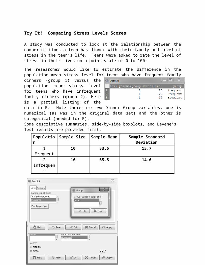
we would expect 75 x (51/150) to prefer vanilla. That is, the expected number of boys

preferring vanilla = (75 )(51 )

150 = ( row total )(column total )Total n . This quick recipe for computing the

expected counts under the null hypothesis is called the Cross-Product Rule.

228

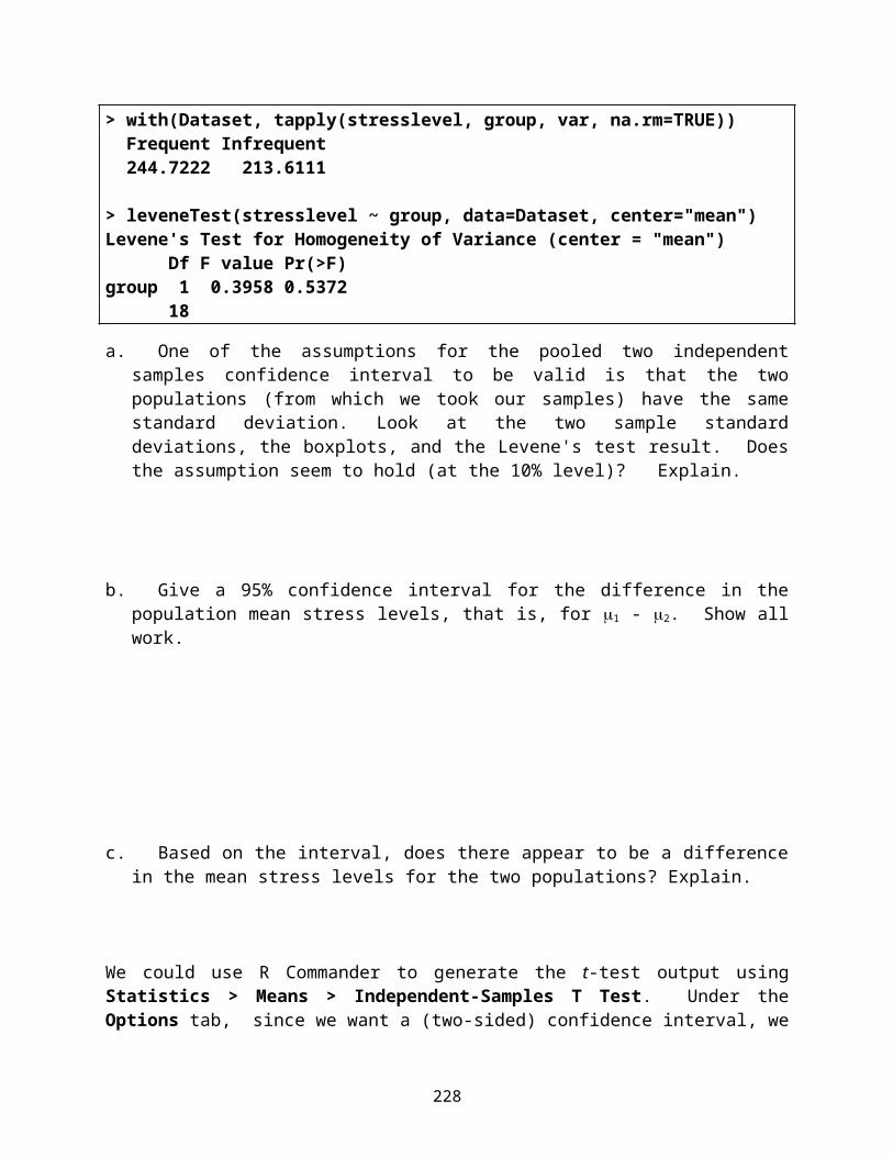
The X2

test statisticNext we need to compute our test statistic, our measure of how close the observed counts are to what we expect under the null hypothesis. Below we are provided the first contribution to the test statistic value. Determine the remaining contributions which are summed to get the value.

X2=(25−25 . 5 )2

25 .5+. ..

The larger the test statistic, the “bigger” the differences between what we observed and what we would expect to see if H0 were true. So the larger the test statistic, the more evidence we have against the null hypothesis.

Is a value of X2= large enough to reject H0?

We need to find the p-value, the probability of getting an X2

test statistic value as large or larger than the one we observed, assuming H0 is true. To do this we need to know the distribution of the X

2 test statistic under the null hypothesis.

If H0 is true, then X2

has the χ2

distribution with degrees of freedom =

Brief motivation for the degrees of freedom formula:

Find the p-value for our ice cream example:

Observed X2

test statistic value = df =

Decision at a 5% significance level: (circle one) Reject H0 Fail to reject H0

Conclusion: It appears that ....

229

Test of Homogeneity Summary (Comparison of Several Populations)

Assume: We have C independent random samples of size n1 ,n2 ,. . ., nc from C populations. We measure 1 discrete response X that has r possible outcomes.

Test: H0: The distribution for the response variable X is the same for all populations.

Test Statistic:X2=∑ (observed - expected )2

expected

where expected =

( row total )(column total )Total n

If H0 is true, then X2

has a χ2

distribution with (r−1)(c−1 ) degrees of freedom. The necessary conditions are: at least 80% of the expected counts are greater than 5 and none are less than 1.

Try It! What is your Decision?For a chi-square test of homogeneity, there are 3 populations and 4 possible values of the discrete characteristic.

If H0 is true, that is, the distribution for the response is the same for all 3 populations, what is the expected value of the test statistic?

230

Try It! Treatment for ShinglesAn article had the headline “For adults, chicken pox vaccine may stop shingles”. A clinical trial was conducted in which 420 subjects were randomly assigned to receive the chicken pox vaccine or a placebo vaccine. Some side effects of interest were swelling and rash around the injection site. Consider the following results for the swelling side effect.

Major Swelling Minor Swelling No SwellingVaccine 54 42 134Placebo 16 32 142

Pearson's Chi-squared test

data: .TableX-squared = 18.5707, df = 2, p-value = 9.277e-05

a. Give the name of the test to be used for assessing if the distribution of swelling status is the same for the two treatment populations.

b. Based on the above data, among those chicken pox vaccinated subjects, what percent had major swelling around the injection site?

c. Based on the above data, among those placebo vaccinated subjects, what percent had major swelling around the injection site?

d. Assuming the distribution of swelling status is the same for the two treatment populations, how many chicken pox vaccinated subjects would you expect to have major swelling around the injection site? Show your work.

e. Compute the contribution to the Chi-square test statistic based on those vaccinated subjects who had major swelling around the injection site.

f. Use a level of 0.05 to assess if the distribution of swelling status is the same for the two treatment populations.Test Statistic Value: ___________ p-value: ______________Thus, the distribution of swelling status (circle your answer): does does not

231

appears to be the same for the two treatment populations.

232

Test of Independence: Helps us to assess if two discrete (categorical) variables are independent for a population, or if there is an association between the two variables.

Test of IndependenceScenario: We have one population of interest - say factory workers.

Question: Is there a relationship between smoking habits and whether or not a factory worker experiences hypertension?

Data: 1 random sample of 180 factory workers, we measure the two variables:Y = hypertension status (yes or no)X = smoking habit (non, moderate, heavy)

The table below summarizes the data in terms of the observed counts.Observed Counts:

X= Smoking Habit Y= Non Mod HeavyHyper Yes 21 36 30Status No 48 26 19

Get the row and column totals.Note: neither row nor column totals were known in advance before measuring hypertension and smoking habit. We only know the overall total of 180.

The null hypothesis:H0: There is no association between smoking habit and hypertension status for the population of factory workers.

(or The two factors, smoking habit and hypertension status, are independent for the population.)

One more mathematical way to write this null hypothesis is:

H0: P (X=i and Y= j )=P( X=i )P(Y= j)

The null hypothesis looks like: P( A and B )=P(A )P(B) , which is one definition of independent events, from our previous discussion of independence.

233

Getting back to our FACTORY WORKERS …The two-way table provides the OBSERVED counts. Our next step is to compute the EXPECTED

counts, under the assumption that H0 is true. The expected counts and the test statistic are found the same way as for the homogeneity test.

Cross-Product Rule: Expected Counts =

( row total )(column total )Total n

Compute and enter these expected counts in the parentheses in the table below.Observed Counts (Expected Counts):

X= Smoking Habit Y= Non Mod HeavyHyper Yes 21

( )36

( )30

( ) 87

Status No 48( )

26( )

19( ) 93

69 62 49 180

The X2

test statisticOur measure of how close the observed counts are to what we expect under the null hypothesis.

X2=(21−33 . 35 )2

33 . 35+.. .

Do you think a value of X2= is large enough to reject H0?

The next step is to find the p-value, the probability of getting an X2

test statistic value as large or larger than the one we observed, assuming H0 is true. To do this we need to know the distribution of the X

2 test statistic under the null hypothesis.

If H0 is true, then X2

has the χ2

distribution with degrees of freedom =_______

Aside: Using our frame of reference for chi-square distributions.If H0 were true, we would expect the X

2 test statistic to be about

give or take about .About how many standard deviations is the observed X

2 value of 14.5 from the expected

value under H0? What do you think the decision will be?

234

235

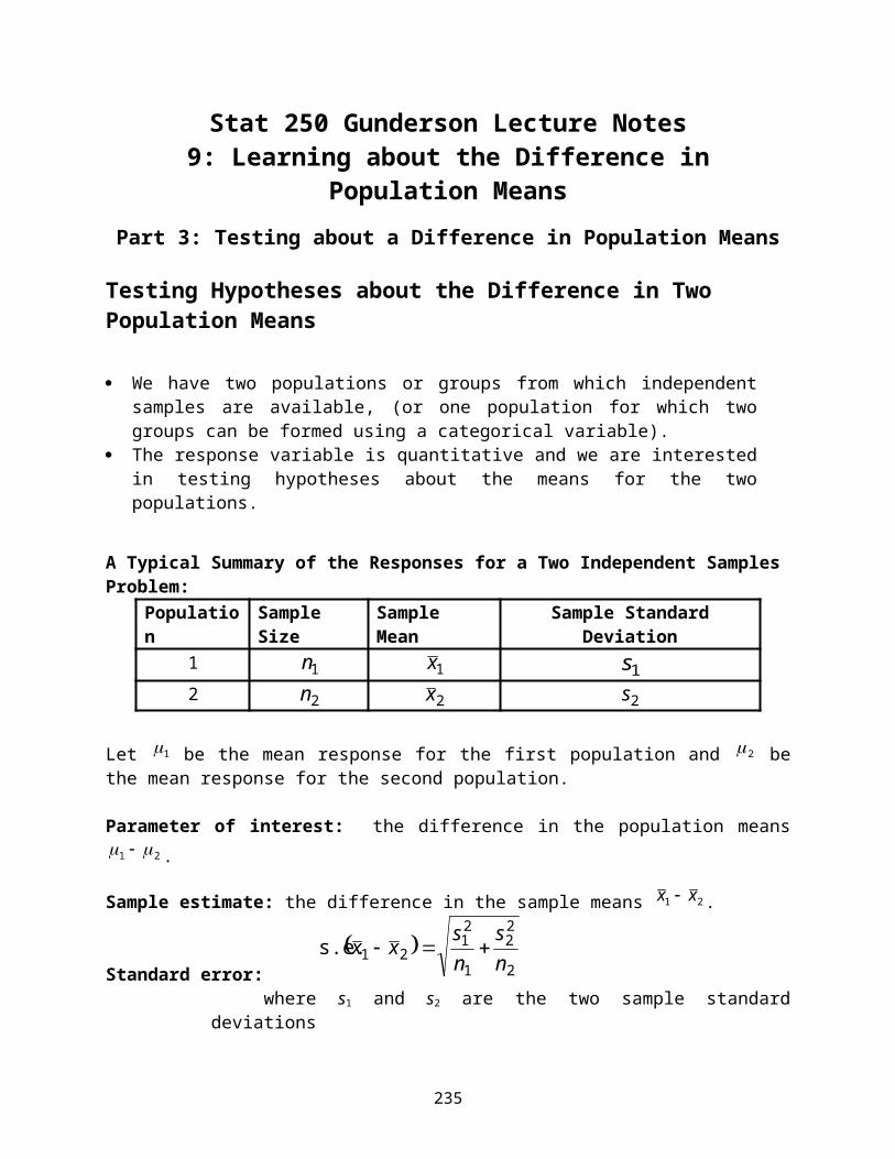
Find the p-value for our factory worker example:

Observed X2

test statistic value = df =

Find the p-value and use it to determine if the results are statistically significant at the 1% significance level.

Conclusion at a 1% level: It appears that ....

Test of Independence Summary

Assume: We have 1 random sample of size n . We measure 2 discrete responses:

X which has r possible outcomes and Y which has c possible outcomes.

Test: H0: The two variables X and Y are independent for the population.

Test Statistic:X2=∑ (observed - expected )2

expected

where expected =

( row total )(column total )Total n

If H0 is true, then X2

has a χ2

distribution with (r−1)(c−1 ) degrees of freedom. The necessary conditions are: at least 80% of the expected counts are greater than 5 and none are less than 1.

236

Relationship between Age Group and Appearance SatisfactionAre you satisfied with your overall appearance? A random sample of 150 women were surveyed. Their answer to this question (very, somewhat, not) was recorded along with their age category (1 = under 30, 2 = 30 to 50, and 3 = over 50).

R was used to generate the following output from the data. Under 30 30 to 50 Over 50Very Satisfied 20 10 16

Somewhat Satisfied 18 20 18Not Satisfied 10 29 9

Pearson's Chi-squared test

data: .TableX-squared = 15.478, df = 4, p-value = 0.003805

a. Give the name of the test to be used for assessing if there is a relationship between age group and appearance satisfaction.

b. Assuming there is no relationship between age group and appearance satisfaction, how many old women (over 50) would you expect to be very satisfied with their appearance?

c. Compute the contribution to the Chi-square test statistic based on the older women (over 50) who were very satisfied with their appearance.

d. Assuming there is no relationship between age group and appearance satisfaction, what is the expected value of the test statistic?

e. Use a level of 0.05 to assess if there is a significant relationship between age group and appearance satisfaction.

Test Statistic Value: _______________ p-value: __________________

Thus, there (circle your answer): does does not

appear to be an association between age group and appearance satisfaction.

237

2x2 Tables – a special case of the two proportion z test The z-test for comparing two population proportions is the same as the chi-square test

provided the alternative is two-sided. The z-test would need to be performed for one-sided alternatives.

When the conditions for the z-test or chi-square test are not met (sample sizes too small) there is another alternative test called the Fisher’s Exact Test.

Stat 250 Formula Card:

Chi-Square TestsTest of Independence &

Test of Homogeneity Test for Goodness of Fit

Expected CountE=expected=row total×column total

total n

Expected CountEi=expected=npi 0

Test Statistic

Χ2=∑ (O−E )2

E=∑ (observed −expected )2

expecteddf = (r – 1)(c – 1)

Test Statistic

Χ2=∑ (O−E )2

E=∑ (observed −expected )2

expecteddf = k – 1

If Y follows a χ2 (df ) distribution, then E(Y) = df and Var(Y) = 2(df).

238

Additional NotesA place to … jot down questions you may have and ask during office hours, take a few extra notes, write out an extra problem or summary completed in lecture, create your own summary about these

concepts.

239