openfoam userconference 2014 berlin · in the next openfoam major release, enhanced ddes methods...
TRANSCRIPT

Copyright © ESI Group, 2013. All rights reserved.Copyright © ESI Group, 2014. All rights reserved.
OpenFoamUserConference 2014
Berlin
October 17, 2014
Copyright © ESI Group, 2014. All rights reserved.
1. DDES enhancements2. SnappyHexMesh Developments3. FoamyHexMesh4. Parallel operation5. Boundedness and MULES
目次

Copyright © ESI Group, 2014. All rights reserved.
DDES Enhancements
After RANS, Detached-Eddy Simulation (DES) is becoming the new standard inindustry:
• Turbulence modelling is the principal accuracy bottleneck in CFD
• DES addresses this by resolving more and modelling less of the turbulent motion
• Enabled by increases in computing power
Copyright © ESI Group, 2014. All rights reserved.
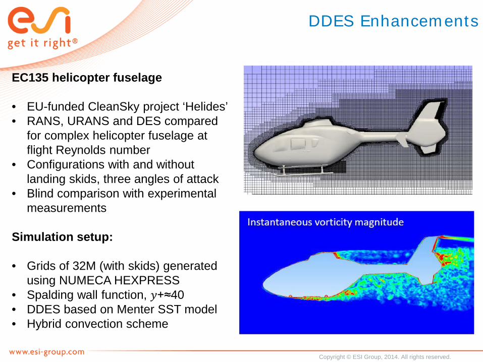
EC135 helicopter fuselage
• EU-funded CleanSky project ‘Helides’• RANS, URANS and DES compared
for complex helicopter fuselage at flight Reynolds number
• Configurations with and without landing skids, three angles of attack
• Blind comparison with experimental measurements
Simulation setup:
• Grids of 32M (with skids) generated using NUMECA HEXPRESS
• Spalding wall function, 𝑦𝑦+≈40• DDES based on Menter SST model• Hybrid convection scheme
DDES Enhancements

Copyright © ESI Group, 2014. All rights reserved.
Prediction of wake topology
• Strong improvement of DES relative to RANS and URANS• Improved prediction of surface pressure in wake region
DDES Enhancements

Copyright © ESI Group, 2014. All rights reserved.
Prediction of wake topology
DDES Enhancements

Copyright © ESI Group, 2014. All rights reserved.
In the next OpenFOAM major release, enhanced DDES methods like SA-WALE-DDES and SA-σ-DDES will be available.
Improved DES methods appear promising:- Improved transition to turbulence in free and separated shear layers - Retains practical and robust nature of approach
DDES Enhancements
Copyright © ESI Group, 2014. All rights reserved.
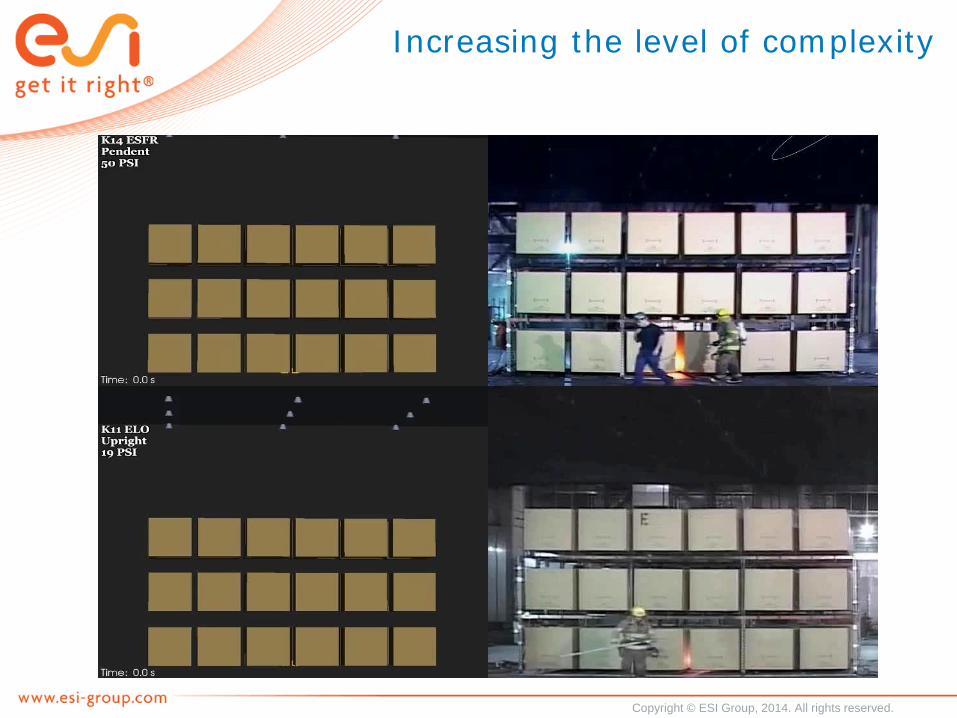
Increasing the level of complexity

Copyright © ESI Group, 2014. All rights reserved.
Increasing the level of complexity

Copyright © ESI Group, 2014. All rights reserved.
Increasing the level of complexity

Copyright © ESI Group, 2014. All rights reserved.
Increasing the level of complexity
Several wind directions are automatically tested to investigate which are the most dangerous wind directions with strong downdraft on the helideck (90% of accidents on oil-rigs are related to helipcoter accidents during landing and take-off).
Copyright © ESI Group, 2014. All rights reserved.
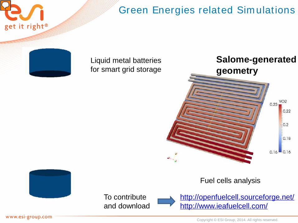
Green Energies related Simulations
Fuel cells analysis
Liquid metal batteries for smart grid storage
http://openfuelcell.sourceforge.net/http://www.ieafuelcell.com/
To contribute and download

Copyright © ESI Group, 2014. All rights reserved.
Green Energies related Simulations
Solar Power Tower
Solver : buoyantPimpleFoam, Radiation: Viewfactor, Turbulence model : k-ω-SST

Copyright © ESI Group, 2014. All rights reserved.
MEXICO project (Model Experiments In Controlled Conditions)
Green Energies related Simulations
Measurements:between June-July 2014 Place:Large Scale Low Speed Facility (LLF) of the German Dutch Wind Tunnels (DNW)Objective:improve the quality of the database

Copyright © ESI Group, 2014. All rights reserved.
SnappyHexMesh OF230 new features
Automatic gap refinement:
• Small gaps will form blockages• Difficult to refine manually• Instead: detect and increase surface refinement level
Copyright © ESI Group, 2014. All rights reserved.
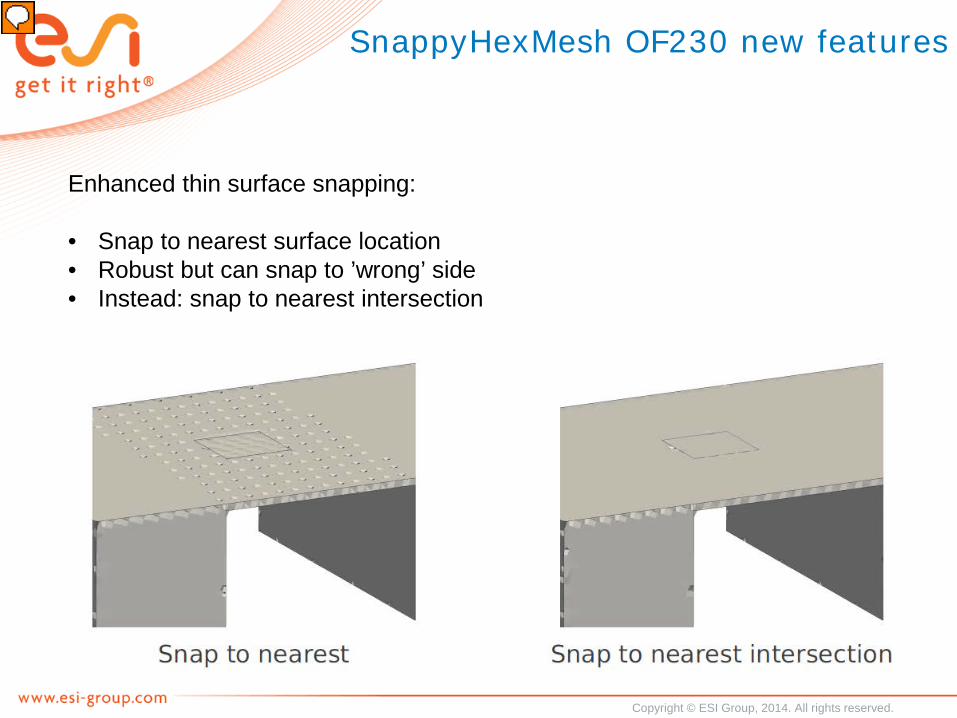
Enhanced thin surface snapping:
• Snap to nearest surface location• Robust but can snap to ’wrong’ side• Instead: snap to nearest intersection
SnappyHexMesh OF230 new features
Copyright © ESI Group, 2014. All rights reserved.
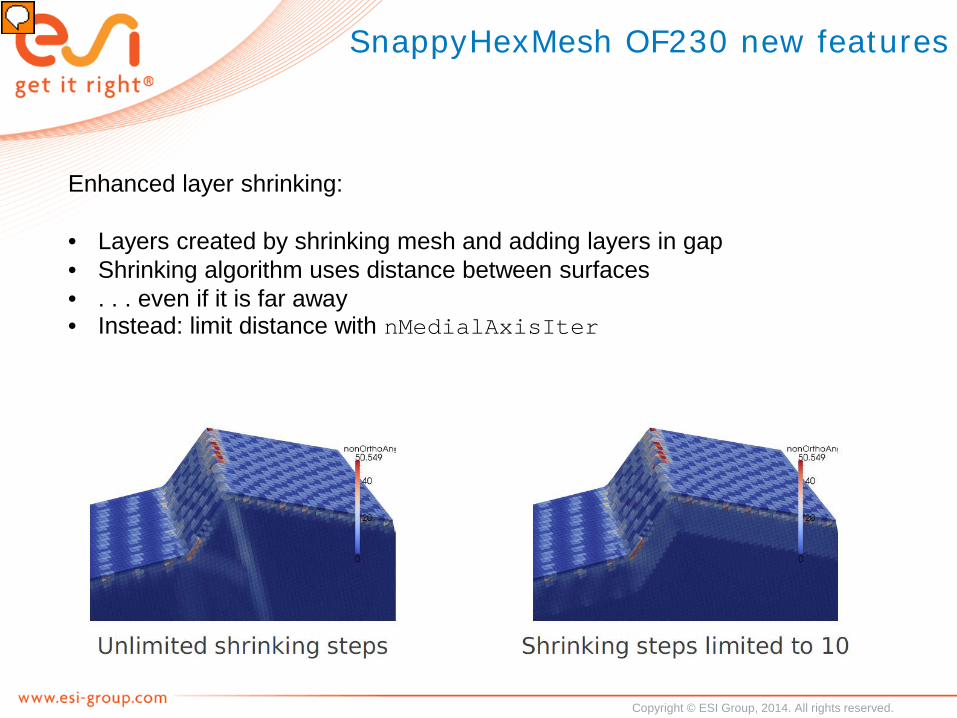
Enhanced layer shrinking:
• Layers created by shrinking mesh and adding layers in gap• Shrinking algorithm uses distance between surfaces• . . . even if it is far away• Instead: limit distance with nMedialAxisIter
SnappyHexMesh OF230 new features

Copyright © ESI Group, 2014. All rights reserved.
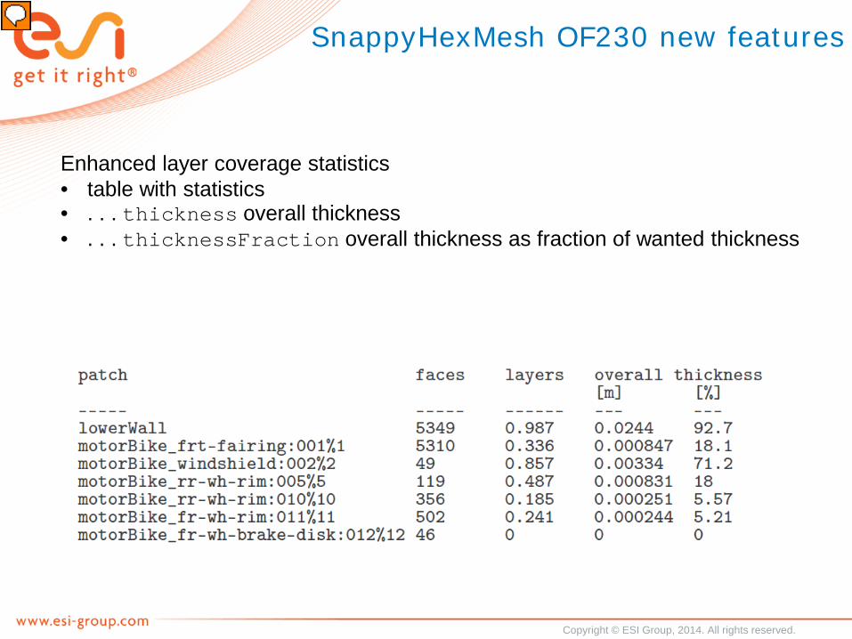
Enhanced layer coverage statistics• fields with boundary values• . . . nSurfaceLayers number of layers• . . . thickness overall thickness• . . . thicknessFraction overall thickness as fraction of wanted thickness
SnappyHexMesh OF230 new features
Copyright © ESI Group, 2014. All rights reserved.
Enhanced layer coverage statistics• table with statistics• . . . thickness overall thickness• . . . thicknessFraction overall thickness as fraction of wanted thickness
SnappyHexMesh OF230 new features
Copyright © ESI Group, 2014. All rights reserved.
In the next major release you can expect:
• Improved multi-region meshing• Improved feature snapping by splitting faces• Ability to add layers to faceZones• Compatibility with dynamic refinement/unrefinement
SnappyHexMesh Current Developments

Copyright © ESI Group, 2014. All rights reserved.
Multi-region meshing• Note: regions are defined using cellZones• . . .with faceZones on region boundaries
Present behaviour• cellZones and faceZones specified through closed surfaces• . . . hard to do nested cellZones• . . . neighbouring cellZones create inconsistent faceZones
New behaviour• specify locationsInMesh (plural)• . . . each location defines a region (cellZone)• . . . faceZones between regions automatically synthesised• . . . optional patchType specification for faceZones• . . . optional locationsOutsideMesh to warn for leaks
SnappyHexMesh Current Developments

Copyright © ESI Group, 2014. All rights reserved.
Multi-region meshing• In practice: nested regions much easier. . .
SnappyHexMesh Current Developments
Copyright © ESI Group, 2014. All rights reserved.
SnappyHexMesh Current Developments
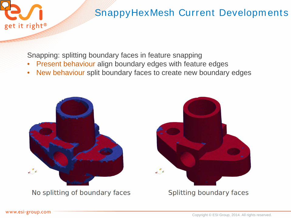
Snapping: splitting boundary faces in feature snapping• Present behaviour align boundary edges with feature edges• New behaviour split boundary faces to create new boundary edges
Copyright © ESI Group, 2014. All rights reserved.
SnappyHexMesh Developments
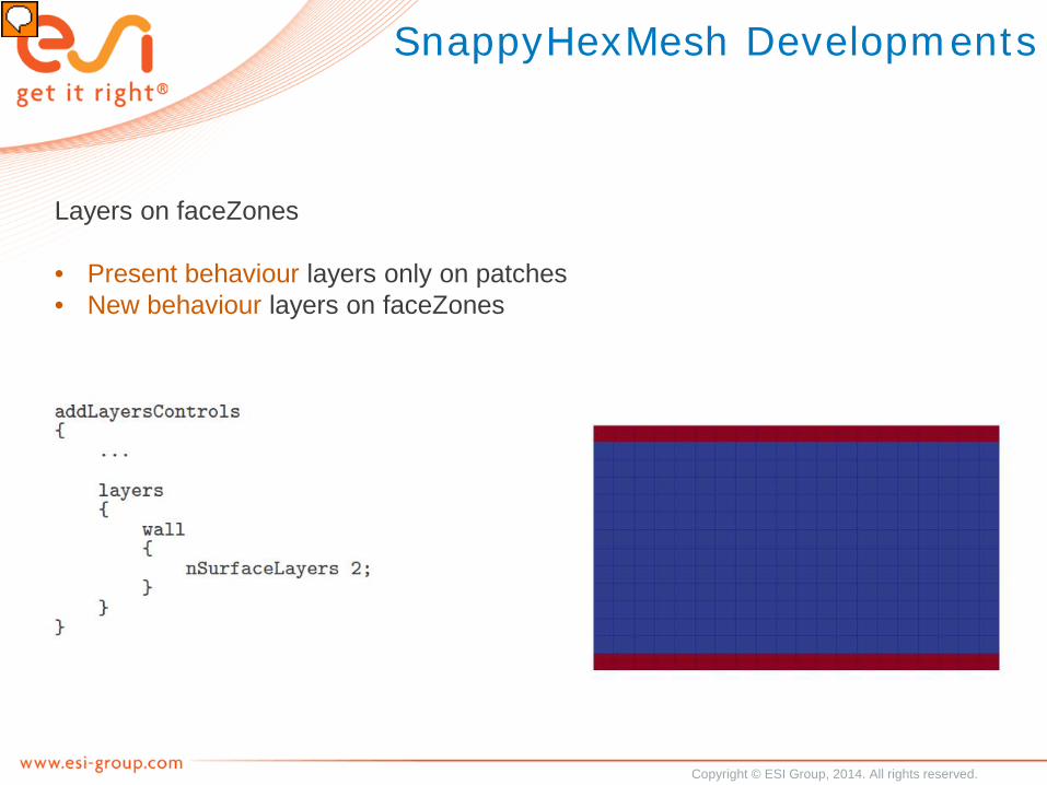
Layers on faceZones
• Present behaviour layers only on patches• New behaviour layers on faceZones

Copyright © ESI Group, 2014. All rights reserved.
SnappyHexMesh Developments
Layers on faceZones
• Present behaviour layers only on patches• New behaviour layers on faceZones
Copyright © ESI Group, 2014. All rights reserved.
SnappyHexMesh Developments
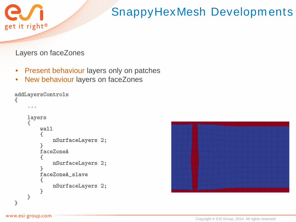
Layers on faceZones
• Present behaviour layers only on patches• New behaviour layers on faceZones

Copyright © ESI Group, 2014. All rights reserved.
SnappyHexMesh Research
Offset surface layer addition: • Layer addition currently uses mesh shrinking
snappyHexMesh layer addition
Copyright © ESI Group, 2014. All rights reserved.
SnappyHexMesh Developments
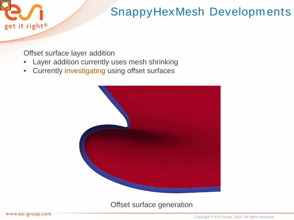
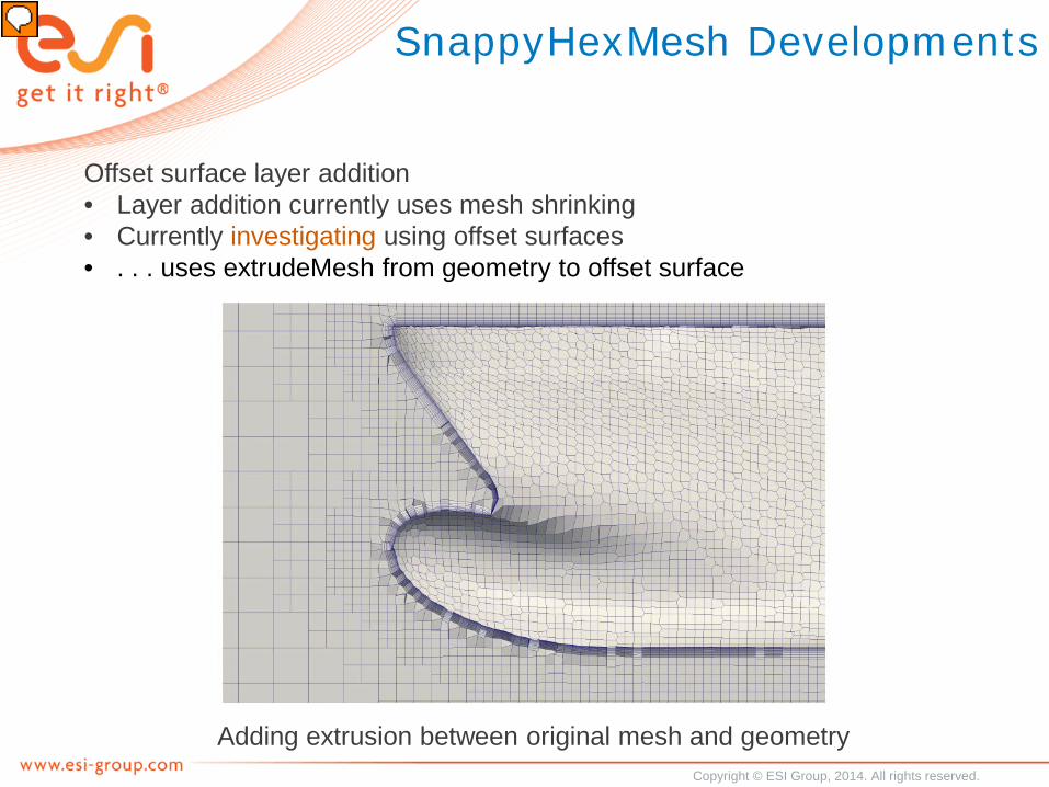
Offset surface layer addition• Layer addition currently uses mesh shrinking• Currently investigating using offset surfaces
Offset surface generation
Copyright © ESI Group, 2014. All rights reserved.
SnappyHexMesh Developments
Offset surface layer addition• Layer addition currently uses mesh shrinking• Currently investigating using offset surfaces• . . . uses extrudeMesh from geometry to offset surface
Adding extrusion between original mesh and geometry

Copyright © ESI Group, 2014. All rights reserved.
foamyHexMesh
• foamyHexMesh fully functional and can be run in parallel• ... requires user evaluation!• Users should find many dictionary inputs familiar e.g. geometry

Copyright © ESI Group, 2014. All rights reserved.
foamyHexMesh
• foamyHexMesh in action. . .
Animation illustrating the point motion algorithm
Copyright © ESI Group, 2014. All rights reserved.
Parallel operation
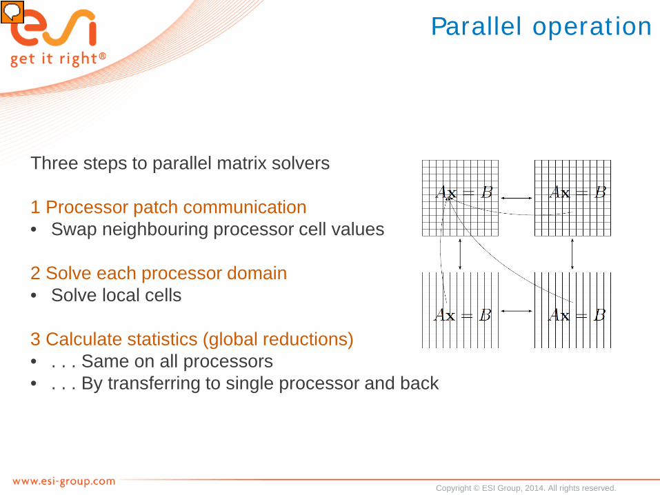
Three steps to parallel matrix solvers
1 Processor patch communication• Swap neighbouring processor cell values
2 Solve each processor domain• Solve local cells
3 Calculate statistics (global reductions)• . . . Same on all processors• . . . By transferring to single processor and back

Copyright © ESI Group, 2014. All rights reserved.
Parallel operation
Use more processors?• Fewer cells per domain, faster to solve?• . . .More communication in steps 1 and 3,• . . .More neighbouring processors,• . . .More processor faces v.s. cells (internal faces),• . . .More explicit meaning worse convergence
Worst case: agglomeration in GAMG solver• Combines (clusters of) cells• Number of cells at coarsest level very low (10?)• Some agglomeration of processor faces• At coarsest level CG solver
• Few cells• With lots of processor faces• Still same cost of global reductions
Copyright © ESI Group, 2014. All rights reserved.
Parallel operation
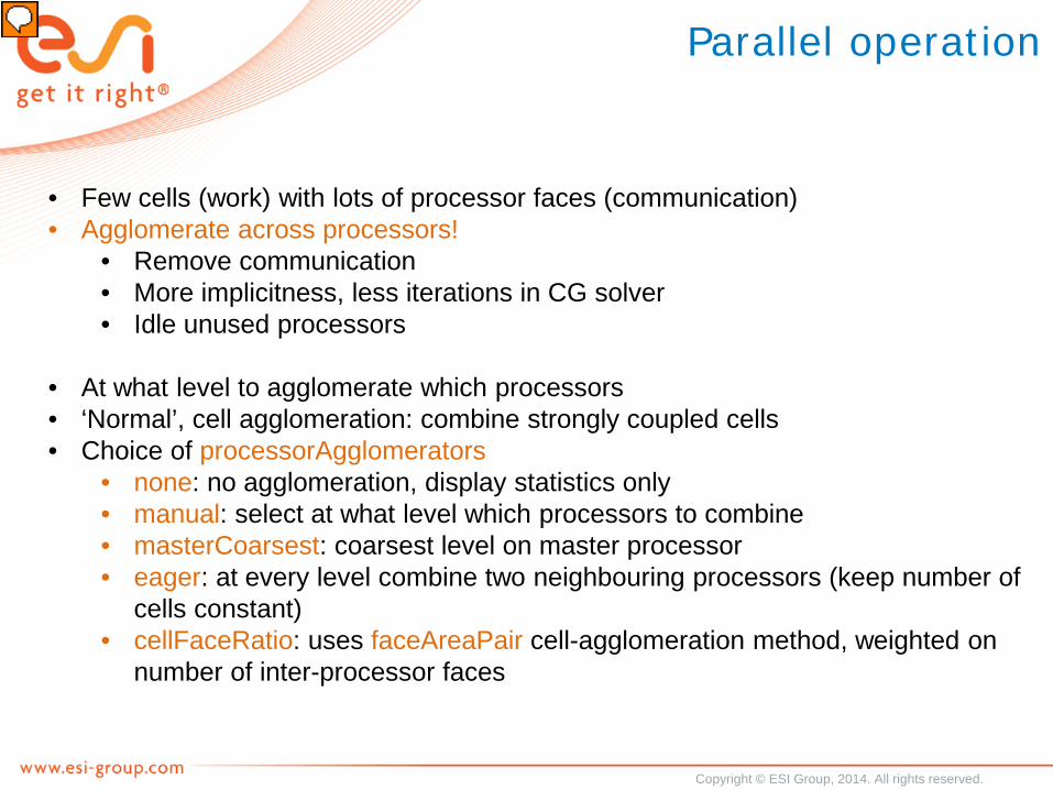
• Few cells (work) with lots of processor faces (communication)• Agglomerate across processors!
• Remove communication• More implicitness, less iterations in CG solver• Idle unused processors
• At what level to agglomerate which processors• ‘Normal’, cell agglomeration: combine strongly coupled cells• Choice of processorAgglomerators
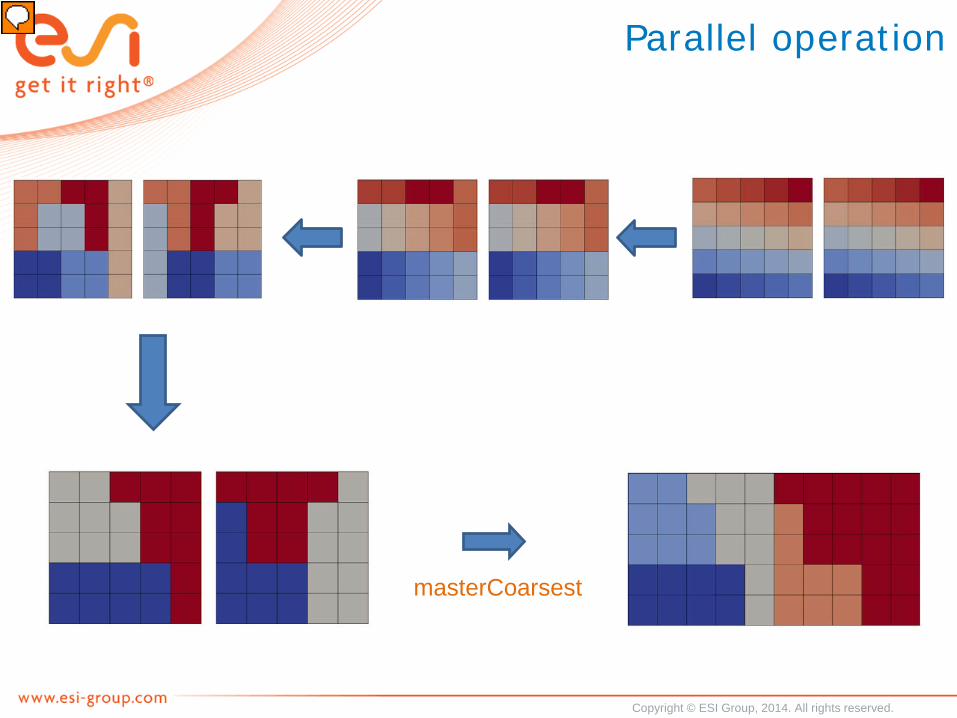
• none: no agglomeration, display statistics only• manual: select at what level which processors to combine• masterCoarsest: coarsest level on master processor• eager: at every level combine two neighbouring processors (keep number of
cells constant)• cellFaceRatio: uses faceAreaPair cell-agglomeration method, weighted on
number of inter-processor faces
Copyright © ESI Group, 2014. All rights reserved.
Parallel operation
masterCoarsest
Copyright © ESI Group, 2014. All rights reserved.
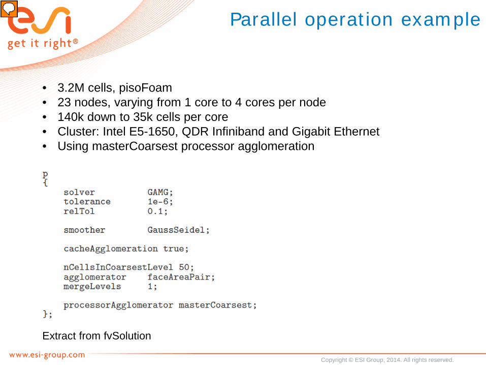
Parallel operation example
• 3.2M cells, pisoFoam• 23 nodes, varying from 1 core to 4 cores per node• 140k down to 35k cells per core• Cluster: Intel E5-1650, QDR Infiniband and Gigabit Ethernet• Using masterCoarsest processor agglomeration
Extract from fvSolution
Copyright © ESI Group, 2014. All rights reserved.
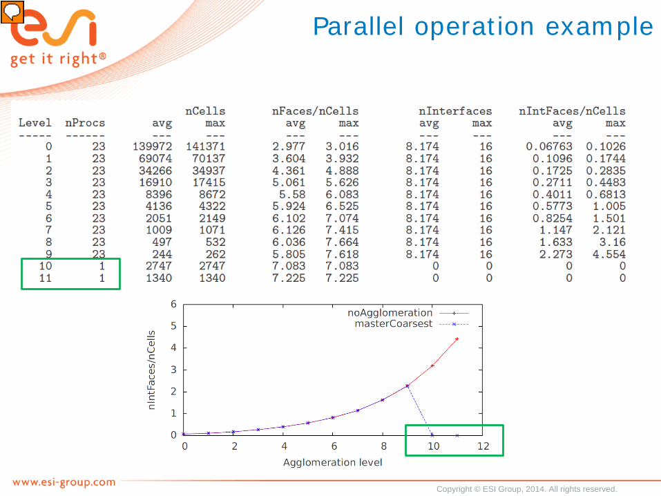
Parallel operation example
Copyright © ESI Group, 2014. All rights reserved.
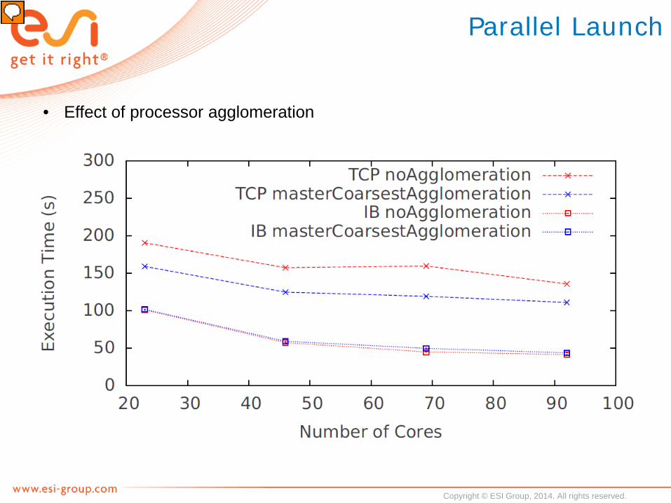
Parallel Launch
• Effect of processor agglomeration

Copyright © ESI Group, 2014. All rights reserved.
Boundedness and MULES
MULES = Multi-dimensional Universal Limiter for Explicit Solution
FVM does not guarantee boundedness.
With MULES we can guarantee boundedness:- MULES explicit with sub-cycling- MULES implicit with limiter iteration- MULES predictor-corrector Recommended and available from OF220- MULES for 2nd-order transport - MULES for 2nd order time... UNDER DEVELOPMENT- MULES for non-orthogonal diffusion correction... UNDER DEVELOPMENT- MULES for coupled variables... UNDER DEVELOPMENT
The future of finite-volume for bounded properties is MULES.
- MULES introduces significant code complexity - requires some core reorganization of OpenFOAM to preserve convenient top-level finite-volume language and to ease maintenance.
Copyright © ESI Group, 2014. All rights reserved.
Final remarks
- All developments will be undertaken on behalf of the OpenFOAM foundation- Copyright transferred to the OpenFOAM Foundation - Released publicly under the GPLv3
For those interested in Discrete Particle Method:
Check MPPICFoam much faster than DPMFoam

Copyright © ESI Group, 2013. All rights reserved.
Thank you for
Your attention