Open Research OnlineThe Open University’s repository of research publicationsand other research outputs

Plio-Pleistocene climate sensitivity evaluated usinghigh-resolution CO2 recordsJournal Item

How to cite:

Martinez-Bot́ı, M. A.; Foster, G. L.; Chalk, T. B.; Rohling, E. J.; Sexton, P. F.; Lunt, D. J.; Pancost, R. D.;Badger, M. P. S. and Schmidt, D. N. (2015). Plio-Pleistocene climate sensitivity evaluated using high-resolution CO2records. Nature, 518(7537) pp. 49–54.

For guidance on citations see FAQs.

c© 2015 Macmillan Publishers Limited.

Version: Accepted Manuscript

Link(s) to article on publisher’s website:http://dx.doi.org/doi:10.1038/nature14145

Copyright and Moral Rights for the articles on this site are retained by the individual authors and/or other copyrightowners. For more information on Open Research Online’s data policy on reuse of materials please consult the policiespage.

oro.open.ac.uk

Plio-Pleistocene climate sensitivity from a new high-resolution CO2 record 1

M.A. Martinez-Boti1,a, G.L. Foster1,a*, T. B. Chalk1, E.J. Rohling2,1, P.F. Sexton3, D.J. Lunt4,5, R.D. 2

Pancost5.6, M.P.S. Badger5,6, D.N. Schmidt5,73

1Ocean and Earth Science, University of Southampton, National Oceanography Centre Southampton, 4

Southampton, SO14 3ZH, UK 5

2Research School of Earth Sciences, The Australian National University, Canberra 2601, Australia 6

3Centre for Earth, Planetary, Space & Astronomical Research, The Open University, Milton Keynes, MK7 6AA, 7

UK 8

4School of Geographical Sciences, University of Bristol, University Road, Bristol, BS8 1SS, UK 9

5The Cabot Institute, University of Bristol, UK 10

6Organic Geochemistry Unit, School of Chemistry, University of Bristol, BS8 1SS, UK 11

7School of Earth Sciences, University of Bristol, Wills Memorial Building, Bristol, BS8 1RJ, UK 12

*corresponding author13

a These authors contributed equally to this work. 14

Theory and climate modelling suggest that the sensitivity of Earth’s climate to changes in radiative 15

forcing could depend on background climate. However, palaeoclimate data have thus far been 16

insufficient to provide a conclusive test of this prediction. Here we present new atmospheric CO2 17

reconstructions based on multi-site boron-isotope records through the late Pliocene (3.3 to 2.3 18

Myr ago). We find that Earth’s climate sensitivity to CO2-based radiative forcing (Earth System 19

Sensitivity) was half as strong during the warm Pliocene as during the cold late Pleistocene (0.8 to 20

0 Myr ago). We attribute this difference to the radiative impacts of continental ice-volume 21

changes (ice-albedo feedback) during the late Pleistocene, because equilibrium climate sensitivity 22

is identical for the two intervals when we account for such impacts using sea-level reconstructions. 23

We conclude that, on a global scale, no unexpected climate feedbacks operated during the warm 24

Pliocene, and that predictions of equilibrium climate sensitivity (excluding long-term ice-albedo 25

feedbacks) for our Pliocene-like future (with CO2 levels up to maximum Pliocene levels of 450 26

ppm) are well described by the currently accepted range of 1.5 to 4.5 K per CO2 doubling. 27

Since the start of the industrial revolution, the concentration of atmospheric CO2 (and other 28

greenhouse gases; GHGs) has increased dramatically (from ~280 to ~400 ppm)1. It has been known 29

for over 100 years that changes in GHG concentration will cause the surface temperature of the 30

Earth to vary2. A wide range of observations reveals that the sensitivity of Earth’s surface 31

temperature to radiative forcing amounts to ~3 K warming per doubling of atmospheric CO2 32

concentration (with a 66% confidence range of 1.5 to 4.5 K; e.g. ref. 1,3), due to direct radiative 33

forcing by CO2 plus the action of a number of fast-acting positive feedback mechanisms, mainly 34

related to atmospheric water vapour content and sea-ice and cloud albedo. Uncertainty in the 35

magnitude of these feedbacks confounds our ability to determine the exact equilibrium climate 36

sensitivity (ECS; the equilibrium global temperature change for a doubling of CO2 on timescales of 37

about a century, when all ‘fast’ feedbacks have had time to operate; see ref. 3 for more detail). 38

Although the likely range of values for ECS is 1.5 to 4.5 K per CO2 doubling, there is a small but finite 39

possibility that climate sensitivity may exceed 5 K (e.g. ref. 1). Understanding the likely value of ECS 40

clearly has important implications for the magnitude, eventual impact and potential mitigation of 41

future climate change. 42

Any long-range forecast of global temperature (i.e. beyond the next 100 years) must also consider 43

the possibility that ECS could depend on the background state of the climate4,5. That is, in a warmer 44

world, some feedbacks that determine ECS could become more efficient and/or new feedbacks 45

could become active to give additional warmth for a given change in radiative forcing (such as those 46

relating to methane cycling6, atmospheric water vapour concentrations5,7,8, in addition to changes in 47

the relative opacity of CO2 to long wave radiation5,9). One approach to identify whether ECS depends 48

on climate background state is to reconstruct ECS during periods in the geological past when Earth 49

was warmer than today. 50

The Pliocene (2.6 to 5.3 Myr ago) is one such time, with the warmest intervals between 3.0 and 3.3 51

Myr ago ~3 K globally warmer than pre-industrial times10,11, while mean sea level stood 12-32 m 52

above the present level12,13. Although most of this warmth is commonly ascribed to increased 53

atmospheric CO2 levels14, it has been suggested that simple comparisons of the observed 54

temperature change in the geological record with the climate forcing from CO2 alone are unable to 55

constrain ECS10. Instead, a parameter termed Earth System Sensitivity (ESS) is defined – the change 56

in global temperature for a doubling of CO2 once both fast and slow feedbacks have acted and the 57

whole Earth system has reached equilibrium (in contrast, ECS excludes the slow feedbacks; for a 58

discussion of fast versus slow feedbacks, see ref. 3). The most important slow feedbacks are those 59

related to ice-albedo and vegetation-albedo changes. Because of these slow feedbacks, Pliocene ESS 60

is thought to have been ~50 % higher than ECS10,15, with some existing geological data suggesting a 61

Pliocene ESS range of 7-10 K per CO2 doubling16, which greatly exceeds a modern ESS estimate of ~4 62

K per CO2 doubling10. If ECS was similarly enhanced, then that would imply that either extra positive 63

fast feedbacks operated, or that existing positive fast feedbacks were more efficient, thus increasing 64

the temperature response for a given level of CO2 forcing. 65

Understanding past climate sensitivity critically depends on the accuracy of the CO2 data used. 66

Despite a tendency toward increased agreement between different CO2 proxies17, individual pCO2 67

estimates for the Pliocene still range from ~190 to ~440 atm (Fig 1a,b) and there is little coherence 68

in the trends described by the various techniques (Fig 1a,b). This hinders any effort to accurately 69

constrain Pliocene ECS or ESS. To better determine Pliocene CO2 levels, we generated a new record, 70

based on the boron isotopic composition (11B) of the surface mixed-layer dwelling planktic 71

foraminiferal species Globigerinoides ruber from ODP Site 999 (Caribbean Sea, 12°44.64’ N, 72

78°44.36’ W, 2838 m water depth; Extended Data Figure 1) at more than 3× higher temporal 73

resolution (1 sample every ~13 kyr; Fig. 1c) than previous 11B records (1 sample every 50 kyr; Fig. 74

1b). The 11B of G. ruber is a well-constrained function of pH18 and seawater pH is well correlated 75

with [CO2]aq, as both are a function of the ratio of alkalinity to total dissolved carbon in seawater. In 76

the absence of significant changes in surface hydrography, [CO2]aq is largely a function of 77

atmospheric CO2 levels and 11B-derived CO2 has been demonstrated to be an accurate recorder of 78

atmospheric CO2 (Extended Data Figure 2a)18-20. Today, the surface water at Site 999 is close to 79

equilibrium with the atmosphere with respect to CO2 (expressed here as pCO2 = pCO2sw-pCO2

atm = 80

+21 atm; Extended Data Figure 1)18,21 and has remained so for at least the last 130 kyr (Extended 81

Data Figure 2)18. ODP Site 999 also benefits from a detailed astronomically calibrated age model22 82

and high abundance of well-preserved planktic foraminifera throughout the past 4 million years23,24. 83

During our study interval it is also unlikely to have been influenced by long-term oceanographic 84

changes such as the emergence of the Panama Isthmus ~3.5 Myr ago (see detailed discussion in ref. 85

23). To increase confidence that atmospheric CO2 changes are driving our pH (and hence our pCO2sw) 86

record for ODP Site 999 and that the air:sea CO2 disequilibrium remained similar to modern values, 87

we also present lower-resolution 11B data from G. ruber from ODP Site 662 (equatorial Atlantic, Fig. 88

1c; 1°23.41’S, 11°44.35°W, 3821 m water depth; Extended Data Figure 1), where current mean 89

annual pCO2 is +29 atm with a seasonal maximum of +41 atm21. Analytical methodology and 90

information detailing precisely how pCO2sw is calculated, with full propagation of uncertainties, can 91

be found in the Methods section (with full 11B and pCO2 in Supplementary Information Tables 1&2). 92

93

A new record of Pliocene pCO2 change 94

Where our data for both sites overlap in time, reconstructed pCO2atm values between 2.3 and 3.3 95

Myr ago agree within uncertainty (Fig 1d; Extended Data Figure 3), and are consistent with most 96

independent records (see Fig 1a,b; Extended Data Figure 2b,c), confirming that the variations we 97

observe are predominantly driven by changes in atmospheric CO2 concentrations. However, the 98

enhanced resolution of our 11B-pCO2atm record (Fig. 1d) also reveals a hitherto 99

undocumented16,23,25,26 level of structure in the CO2 variability during the 1 million year period 100

investigated, including a transition centred on 2.8 Ma, spanning ~200 kyr, where average pCO2atm 101

undergoes a decrease of ~65 atm (Fig 1d). 102

Detailed atmospheric CO2 measurements from ice cores show orbital-scale (~100 kyr) oscillations in 103

pCO2atm with a peak-to-trough variation of ~80-100 atm through the late Pleistocene (90 % of the 104

pCO2 values lie between +36 and –41 atm of the long-term mean; Extended Data Figures 2, 4)27-29. 105

Once the long-term trend is removed from our Plio-Pleistocene data (thick blue line in Fig 1d), and 106

we have taken into account our larger analytical uncertainty (see Methods), we observe orbital-scale 107

variations in our 11B-pCO2atm record of only slightly smaller amplitude than the ice-core pCO2

atm 108

record (0-0.8 Myrs) and for the last 2 Myrs in other 11B-based records19,20,30 (Extended Data Figure 4 109

and Methods), which is in clear contrast with the benthic 18O which shows increasing variability 110

over the last 3 Myrs (Fig 1e and Extended Data Figure 4). 111

Given the different amplitudes of climate variability, the observed similarity between Pliocene and 112

late Pleistocene pCO2atm variability seems counter-intuitive given the notion that CO2 is a key factor 113

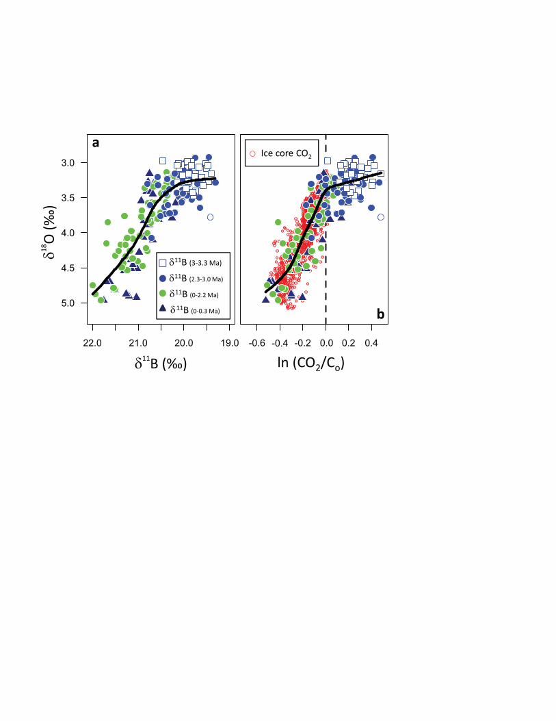
in amplifying glacial-interglacial climate change27-29,31,32. This is illustrated by a well-defined non-114

linear relationship in a cross plot between deep-sea benthic 18O and ln(CO2/Co) (where Co = pre-115

industrial CO2 = 278 atm), which accounts for the logarithmic nature of the climate forcing by CO2 116

(Fig. 2b). Note also the clear overlap between Pleistocene (0-2.2 Myrs) ice-core CO2 measurements 117

and 11B-based CO2 reconstructions in this plot (Fig. 2b; Extended Data Figure 2). A similar 118

relationship is also evident in raw 11B-space (Fig. 2a). Below an inflection at about 275±15 atm 119

pCO2atm (equating to ln(CO2/Co) ≈ 0) benthic 18O shows a steeper relationship with CO2-based 120

forcing than it does above this value (Fig. 2). This likely reflects some combination of: (i) growth of 121

larger northern hemisphere ice sheets at pCO2atm

below 275±15 atm33 increasing radiative ice-122

albedo feedback and amplifying climate forcing by CO2 change; (ii) an increase in oxygen isotope 123

fractionation in precipitation with increasing size of the ice sheets, which leads to a proportionally 124

greater 18O enrichment in seawater34; and (iii) potentially stronger deep-sea cooling at low pCO2atm 125

due to the high-latitude-focussed influences of the ice-albedo feedback process. These findings 126

highlight the profound impacts of northern hemisphere ice-sheet growth on climate variability in the 127

Pleistocene 31,32, relative to the Pliocene (Fig. 2b). 128

Our new data show that the ~275±15 atm threshold was first crossed at ~2.8 Ma during Marine 129

Isotope Stage (MIS) G10 (Fig. 1d, horizontal dashed line), and – more persistently – during 130

subsequent Marine Isotope Stages G6 (2.72 Myr ago), G2 (2.65 Myr ago), and 100 (2.52 Myr ago), 131

when values as low as atm (95% confidence) were reached and when intervening 132

interglacial values also seem to have been suppressed (Fig. 1c,d). These isotope stages are significant 133

in that they are associated with an increase in the amplitude of glacial-interglacial sea-level 134

oscillations (Extended Data Figure 5b)12,13,35 and coincide with the timing of the first substantial 135

continental glaciations of Europe, North America and the Canadian Cordillera, as reconstructed by 136

Ice-rafted debris and observations of relic continental glacial deposits36-38. Hence, our new high-137

resolution pCO2atm record robustly confirms previous hypotheses16,23,25,39 (based on low-resolution 138

CO2 data) that the first substantial stages of glaciation on the northern hemisphere, as well as a 139

recently recognised deep-sea cooling during the late Pliocene/early Pleistocene13, coincided with a 140

significant decline in mean atmospheric pCO2atm at 2.7-2.9 Ma of ~40-90 µatm (mean3.0-3.2Ma – 141

mean2.4-2.7Ma = 66 ± 26 µatm; p <0.001 (two-tailed), n=40). 142

143

Efficiency of climate feedbacks 144

The high fidelity of the boron isotope pH/pCO2atm proxy (Extended Data Figure 2), coupled with the 145

high resolution of our new pCO2atm record, offers an opportunity to examine the sensitivity of Earth’s 146

climate system to forcing by CO2 during a period when Earth’s climate was, on average, warmer than 147

today40. For this exercise, global temperature estimates are also needed. We consider two 148

approaches for this. The first is an estimate of global mean annual surface air temperature change 149

(MAT) over the last 3.5 million years, from a scaling of the northern hemisphere climate required 150

to drive an ice-sheet model to produce deep ocean temperature and ice-volume changes consistent 151

with benthic 18O data (Fig 3a,b)35. This approach produces a continuous record of global 152

temperature that agrees well with independent constraints for discrete time intervals (see ref. 35). 153

We supplement MAT with a record from a second approach, which is independent from benthic 154

18O values. For this, we generated a sea surface temperature stack (SSTst) from 0 to 3.5 Myr ago 155

(Fig. 3c,d), comprising 10 high-resolution (average ~4 kyr) SST records based on Uk’37 alkenone 156

unsaturation ratios, from latitudes between 41 oS and 57 oN. The selected sites (see Extended Data 157

Figure 1b) all offer near-continuous temporal coverage of the last 3.5 Myr (see Methods). Our SSTst 158

record agrees well with independent, higher density compilations of global SST change32,41 (Fig 3c 159

blue line), indicating that SSTst offers a reliable approximation of global SST change (see Methods for 160

more details). Moreover, our SSTst allows us to directly compare the major SST changes, within the 161

same archives, between the Plio-Pleistocene and late Pleistocene. 162

When comparing temperature records from the two approaches considered, it must be emphasized 163

that MAT reflects global mean annual surface air temperature change, while SSTst approximates 164

global mean sea surface temperature change. Hence, their amplitudes of variability will be different, 165

mainly because SSTst does not include temperature changes over land. Approximately, SST = MAT 166

* 0.66 (ref. 32,42), but direct conversion is not needed here, as we merely aim to contrast Pliocene 167

climate behaviour with that for the Pleistocene, within the same data types. 168

To determine the sensitivity of global SST and MAT to CO2 forcing in the Pliocene and Pleistocene, 169

we use time series of forcing calculated from our new and existing CO2 records (Fig 3e to h), and 170

regress these against both MAT and SSTst (Fig 3a to d; Supplementary Information Tables 1-3). The 171

regression slopes then describe the average temperature change (T in K) per W per m2 of forcing 172

(F) for each time interval. These gradients therefore approximate the commonly used sensitivity 173

parameter (S = T/F K W-1 m2) for describing global temperature change for a given forcing3. In this 174

scheme, a doubling of atmospheric CO2 is equivalent to a forcing of 3.7 W m-2, so that for the 66% 175

confidence interval of modern climate sensitivity quoted by ref. 1, the present-day equilibrium value 176

of S (Sa, after ref. 3) is 1.5/3.7 to 4.5/3.7 = 0.4 to 1.2 K W-1 m2. However, using palaeoclimate data it 177

is not possible to determine the direct equivalent of Sa; instead, such studies constrain a ‘past’ 178

parameter (Sp), which includes the combined action of both fast and slow feedbacks3. Note that 179

Earth System Sensitivity, ESS (in K) = Sp x 3.7. Explicit accounting for slow feedback processes in 180

determinations of Sp can make it approximate Sa (ref. 3). Following ref. 3, an Sp estimate after 181

accounting for carbon-cycle feedback is indicated by SCO2, and one accounting for both carbon-cycle 182

and land-ice-albedo feedbacks is SCO2,LI, where the latter gives a useful approximation of Sa. We 183

follow this approach, using Sp = MAT/F and Sp,SSTSST/F, both in K W-1 m2. Note that our 184

determinations of the sensitivity parameter are based on our entire reconstructed time series, 185

rather than on a simple comparison between a limited Pliocene average and the modern average, as 186

was done in previous studies3,16. Since we calculate a Sp (and Sp,SST) for the Pliocene and compare this 187

to the late Pleistocene Sp (and Sp,SST), we also avoid complications due to independent changes in 188

boundary conditions (such as topographic changes)39 because we assess sensitivity within each 189

relatively short time window (2.3 to 3.3 Ma vs. 0 to 0.8 Ma). In addition, our approach emphasizes 190

relative changes in CO2 levels and temperature over the intervals considered, rather than absolute 191

values. This improves accuracy because relative changes are much better constrained than absolute 192

temperature and pCO2atm values from proxy data (see Methods for further discussion). 193

Preliminary regression of MAT against Pliocene pCO2atm identified one data point (at 2362 kyr; 194

white circle in Fig. 1d & 2) with a particularly large residual and significant leverage on the least 195

squares regression (a high Cook’s distance). With interglacial-like pCO2atm values but glacial-like 18O 196

values (Fig 2), this point may reflect a chronological error, or a short period of unusually high air:sea 197

disequilibrium with respect to CO2 at ODP Site 999. To avoid the influence of this one point on 198

subsequent linear regressions, we have removed it from our 11B-pCO2atm record. The remaining 199

pCO2atm data (73 points) were interpolated to a constant resolution (1 kyr), smoothed with a 20 kyr 200

moving average to reduce short-term noise and resampled back to the original data spacing (~1 201

sample every 13 kyr). A Monte Carlo approach was followed to determine uncertainties for this 202

smoothed record given the uncertainty in the 11B-derived pCO2atm. Radiative forcing changes due to 203

pCO2atm changes are calculated using FCO2 = 5.35*ln(CO2/Co) W m-2; where Co = 278 atm (Fig 3)43. 204

We ignore mean annual forcing by orbital variations because it is small (<0.5 W m-2 with a periodicity 205

of 100 to 400 kyr)31,32 and averages out over the length of our records. Linear regressions of MAT 206

and SSTst versus FCO2 were performed using an approach that yields a probabilistic estimate of 207

slope, and hence sensitivity to CO2 forcing (SCO2 = T/FCO2 or SCO2,LI = T/FCO2,LI), which fully 208

accounts for uncertainties in both X and Y variables (see Methods; Fig 4). Fig 5a-d displays 209

probability distribution functions (pdfs) of the determinations of slope for each time interval. This 210

analysis reveals that, irrespective of the global temperature record used (MAT or SSTst), the 211

average global sensitivity of Earth’s climate to forcing by CO2 only (SCO2) is approximately 2x higher 212

for the Pleistocene than it is for the Pliocene (Fig 4&5). This validates previous inferences of a strong 213

additional feedback factor during the Pleistocene (at pCO2atm levels below ~280 atm), which likely 214

arises from the growth and retreat of large northern hemisphere ice sheets and their role in 215

changing global albedo31,32. 216

Given that, to a first order, the Earth system responds to radiative forcing in a consistent fashion, 217

largely independent of the nature of that forcing8, we can determine the climate forcing arising from 218

continental ice albedo changes via a relatively simple parameterisation of sea-level change (FLI = 219

sea-level change (m) × 0.0308 W m-2; following ref. 31,32). Several reconstructions of sea-level 220

change partially or completely span the last 3.5 Ma (e.g., ref. 13, 35, 44, 45, and 46 recalculated by 221

12), and we explore the implications of each of these independent records. Cross-plots of combined 222

CO2 and ice-albedo forcing (FCO2 + FLI = FCO2,LI) versus MAT and SSTst are shown in Fig 4 for the 223

Pliocene and Pleistocene. Fig 5e-h displays the influence of choices of temperature and sea-level 224

record on our determinations of SCO2,LI (= T/FCO2,LI). In contrast to SCO2, SCO2,LI is similar for both the 225

Pliocene and Pleistocene, regardless of temperature record or other parameter choices (Fig 5). This 226

robustly indicates that the apparent difference between Pliocene and Pleistocene climate sensitivity 227

arises almost entirely from ice-albedo feedback influences. It also implies that all of the other 228

feedbacks that amplify climate forcing by CO2 (e.g. sea-ice and cloud albedo, water vapour, 229

vegetation, aerosols, other GHGs) must have operated with rather similar efficiencies during both 230

the Pliocene and Pleistocene. Thus, we find no evidence that additional (unexpected) positive 231

feedbacks had become active to amplify Earth system sensitivity to CO2 forcing during the warm 232

Pliocene. Alternatively, if additional positive feedbacks did become active (e.g. increase in steady-233

state methane concentration or changes in cloud properties), then their effect must have been 234

negated by the loss of other amplifying feedbacks (e.g. Arctic sea-ice) or the addition of more 235

negative feedbacks. This finding is at odds with previous studies (e.g. ref. 16,47) most likely because 236

of differences in our approach to determine Pliocene climate sensitivity (i.e. we determine a within-237

Pliocene sensitivity) and shortcomings in the proxy systems used by the earlier investigations, both 238

in terms of CO2 and temperatures (e.g. see ref. 48). For instance, Fig 1d (and Extended Data Figure 239

2) indicate that both orbital-scale variability in pCO2atm and the major decline at 2.7-2.9 Ma are 240

absent from the previously used16 alkenone-based pCO2atm records and as a result regressions of 241

temperature and alkenone-derived forcing are poorly defined (Extended Data Figure 2d-f). 242

243

Constraints on Climate Sensitivity 244

Using the geological record to directly estimate ECS (and thus Sa) is problematic because information 245

on the appropriate magnitude of a number of key feedbacks (such as vegetation-albedo) is typically 246

unavailable3. Nonetheless, considerable effort has determined that ECS estimates based on the last 247

glacial maximum fall within the range of ECS estimates from other approaches (1.5 to 4.5 K per CO2 248

doubling, or 0.4 to 1.2 K W-1 m2; ref. 1). Our analysis implies that a similar ECS applies to the Pliocene 249

and early Pleistocene (2.3 to 3.3 Ma; Fig 5; Supplementary Information Table 4). In addition, our 250

estimate of Pliocene SCO2 using MAT lies within a range of 0.6 to 1.5 K W-1 m2 (at 95% confidence), 251

meaning that, once all feedbacks have played out for future CO2 doubling, ESS (= SCO2 x 3.7) will very 252

likely (95% confidence) be <5.2 K and will likely (68% confidence) fall within a range of 3.0 to 4.4 K 253

(Supplementary Information Table 4). 254

In May 2013, atmospheric CO2 levels crossed the 400 ppm threshold to values last seen during the 255

Pliocene (Fig. 1c). Given current CO2 emission rates, global temperatures may reach those typical of 256

the warm periods of the Pliocene by 20501. Our findings suggest that, if the Earth system behaves in 257

a similar fashion to how it did during the Pliocene as it continues to warm in the coming years, an 258

ECS of 1.5 to 4.5 K per CO2 doubling1 likely provides a reliable description of the Earth’s temperature 259

response to climate forcing, at least for global temperature rise up to 3 K above the pre-industrial 260

level. Studies of even warmer intervals in the deeper geological past (well before 3.3 Myr ago) are 261

needed to determine whether any additional climate feedbacks should be expected as the Earth 262

warms even further into the 22nd Century if CO2 emissions continue unabated. 263

264

References 265

1 IPCC, 2013: Climate Change 2013: The Physical Science Basis. Contribution of Working Group 266

I to the Fifth Assessment Report of the Intergovernmental Panel on Climate Change [Stocker, T.F., D. 267

Qin, G.-K. Plattner, M. Tignor, S.K. Allen, J. Boschung, A. Nauels, Y. Xia, V. Bex and P.M. Midgley 268

(eds.)]. Cambridge University Press, Cambridge, United Kingdom and New York, NY, USA, 1535 pp 269

(2013). 270

2 Arrhenius, S. On the influence of carbonic acid in the air upon the temperature of the 271

ground. Philosphical Magazine and Journal of Science 5, 237-276 (1896). 272

3 Rohling, E. J. et al. Making sense of palaeoclimate sensitivity. Nature 491, 683-691, 273

doi:10.1038/nature11574 (2012). 274

4 Crucifix, M. Does the Last Glacial Maximum constrain climate sensitivity? Geophys. Res. Lett. 275

33, doi:10.1029/2006GL027137, 022006 (2006). 276

5 Caballero, R. & Huber, M. State-dependent climate sensitivity in past warm climates and its 277

implication for future climate projections. PNAS, 110 (35), 14162-278

14167doi:www.pnas.org/cgi/doi/10.1073/pnas.1303365110 (2013). 279

6 Beerling, D. J., Fox, A., Stevenson, D. S. & Valdes, P. J. Enhanced chemistry-climate feedbacks 280

in past greenhouse worlds. PNAS 108, 9770-9775, doi: 10.1073/pnas.1102409108 (2011). 281

7 Meraner, K., Mauritsen, T. & Voigt, A. Robust increase in equilibrium climate sensitivity 282

under global warming. Geophys. Res. Lett. 40, 5944-5948, doi:10.1002/2013GL058118 (2013). 283

8 Hansen, J. et al. Efficacy of climate forcings. J. Geophys. Res. 110, 284

doi:10.1029/2005JD005776 (2005). 285

9 Byrne, B. & Goldblatt, C. Radiative forcing at high concentrations of well-mixed greenhouse 286

gases. Geophys. Res. Lett.41, 152-160, doi:10.1002/2013GL058456. (2013). 287

10 Lunt, D. J. et al. Earth system sensitivity inferred from Pliocene modelling and data. Nature 288

Geoscience 3, 60-64, doi:10.1038/NGEO706 (2010). 289

11 Haywood, A. M. & Valdes, P. J. Modelling Pliocene warmth: contribution of atmosphere, 290

oceans and cryosphere. Earth Planet. Sci. Lett. 218, 363-377 (2004). 291

12 Miller, K. G. et al. High tide of the warm Pliocene: Implications of global sea level for 292

Antarctic deglaciation. Geology 40, 407-410, doi:10.1130/G32869.1 (2012). 293

13 Rohling, E. J. et al. Sea-level and deep-sea-temperature variability over the past 5.3 million 294

years. Nature 508, 477-482, doi:10.1038/nature13230 (2014). 295

14 Lunt, D. J. et al. On the causes of mid-Pliocene warmth and polar amplification. Earth Planet. 296

Sci. Lett. 321-322, 128-138, doi:10.1016/j.epsl.2011.12.042 (2012). 297

15 Haywood, A. M. et al. Large-scale features of Pliocene climate: results from the Pliocene 298

Model Intercomparison Project. Clim. Past 9, 191-209, doi:10.5194/cp-9-191-2013 (2013). 299

16 Pagani, M., Liu, Z., LaRiviere, J. & Ravelo, A. C. High Earth-system climate sensitivity 300

determined from Pliocene carbon dioxide concentrations. Nature Geoscience 3, 27-30, doi:DOI: 301

10.1038/NGEO724 (2010). 302

17 Beerling, D. J. & Royer, D. L. Convergent Cenozoic CO2 history. Nature Geoscience 4, 418-420, 303

doi:10.1038/ngeo1186 (2011). 304

18 Henehan, M. J. et al. Calibration of the boron isotope proxy in the planktonic foraminifera 305

Globigerinoides ruber for use in palaeo-CO2 reconstruction. Earth Planet. Sci. Lett. 364, 111-122, 306

doi:10.1016/j.epsl.2012.12.029 (2013). 307

19 Hönisch, B. & Hemming, N. G. Surface ocean pH response to variations in pCO2 through two 308

full glacial cycles. Earth Planet. Sci. Lett. 236, 305-314 (2005). 309

20 Foster, G. L. Seawater pH, pCO2 and [CO32-] variations in the Caribbean Sea over the last 130 310

kyr: A boron isotope and B/Ca study of planktic foraminifera. Earth Planet. Sci. Lett. 271, 254-266 311

(2008). 312

21 Takahashi, K. et al. Climatological mean and decadal change in surface ocean pCO2, and net 313

sea-air CO2 flux over the global oceans. Deep-Sea Res. II 56, 554-577 (2009). 314

22 Lisiecki, L. E. & Raymo, M. E. A Pliocene-Pleistocene stack of 57 globally distributed benthic 315

18O records. Paleoceanography 20, doi: 10.1029/2004PA001071 (2005). 316

23 Bartoli, G., Hönisch, B. & Zeebe, R. Atmospheric CO2 decline during the Pliocene 317

intensification of Northern Hemisphere Glaciations. Paleoceanography 26, PA4213, 318

doi:4210.1029/2010PA002055 (2012). 319

24 Davis, C.V., Badger, M.P.S., Bown, P.R. & Schmidt, D.N. The response of calcifying plankton 320

to climate change in the Pliocene, Biogeosciences, 10, 6131-6139 (2013). 321

25 Seki, O. et al. Alkenone and boron based Plio-Pleistocene pCO2 records. Earth Planet. Sci. 322

Lett. 292, 201-211 (2010). 323

26 Badger, M. P. S., Schmidt, D. N., Mackensen, A. & Pancost, R. D. High resolution alkenone 324

palaeobarometry indicates relatively stable pCO2 during the Pliocene (3.3 to 2.8 Ma). Philos. Trans. 325

Royal Soc. A 347, 20130094, doi: 10.1098/rsta.2013.0094 (2013). 326

27 Petit, J. R. et al. Climate and atmospheric history of the past 420,000 years from the Vostok 327

ice core, Antarctica. Nature 399, 429-436 (1999). 328

28 Lüthi, D. et al. High-resolution carbon dioxide concentration record 650,000-800,000 years 329

before present. Nature 453, 379-382, doi:10.1038/nature06949 (2008). 330

29 Siegenthaler, U. et al. Stable carbon cycle-climate relationship during the Late Pleistocene. 331

Science 310, 1313-1317 (2005). 332

30 Hönisch, B., Hemming, G., Archer, D., Siddal, M. & McManus, J. Atmospheric carbon dioxide 333

concentration across the Mid-Pleistocene Transition. Science 324, 1551-1554 (2009). 334

31 Köhler, P. et al. What caused Earth's temperature variations during the last 800,000 years? 335

Data-based evidence on radiative forcing and constraints on climate sensitivity. Quat. Sci. Reviews 336

29, 129-145, doi:10.1016/j.quascirev.2009.09.026 (2010). 337

32 Rohling, E. J., Medina-Elizalde, M., Shepherd, J. G., Siddall, M. & Stanford, J. D. Sea surface 338

and High-lattitude temperature sensitivity to radiative forcing of climate over several glacial cycles. 339

J. Climate 25, 1635-1656, doi:10.1175/2011JCLI4078.1 (2012). 340

33 DeConto, R. M. et al. Thresholds for Cenozoic bipolar glaciation. Nature 455, 652-656 (2008). 341

34 Shackleton, N. Oxygen isotope analyses and Pleistocene temperatures re-assessed. Nature 342

215, 15-17 (1967). 343

35 van de Wal, R. S. W., de Boer, B., Lourens, L. J., Köhler, P. & Bintanja, R. Reconstruction of a 344

continuous high-resolution CO2 record over the past 20 million years Clim. Past 7, 1459-1469, 345

doi:10.5194/cp-7-1459-2011 (2011). 346

36 Balco, G. & Rovey, C. W., II. Absolute chronology for major Pleistocene advances of the 347

Laurentide Ice Sheet. Geology 38, 795-798, doi:10.1130/G30946.1 (2010). 348

37 Bailey, I. et al. An alternative suggestion for the Pliocene onset of major northern 349

hemisphere glaciation based on geochemical provenance of North Atlantic Ocean ice-rafted debris. 350

Quat. Sci. Reviews 75, 181-194, doi:10.1016/j.quascirev.2013.06.004 (2013). 351

38 Hidy, A. J., Gosse, J. C., Froese, D. G., Bond, J. D. & Rood, D. H. A latest Pliocene age for the 352

earliest and most extensive Cordilleran Ice Sheet in northwestern Canada. Quat. Sci. Reviews 61, 77-353

84, doi:10.1016/j.quascirev.2012.11.009 (2013). 354

39 Lunt, D. J., Foster, G. L., Haywood, A. M. & Stone, E. J. Late Pliocene Greenland glaciation 355

controlled by a decline in atmospheric CO2 levels. Nature 454, 1102-1105 (2008). 356

40 Dowsett, H. J. et al. Assessing confidence in Pliocene sea surface temperatures to evaluate 357

predictive models. Nature Climate Change 2, 365-371, doi:10.1038/NCLIMATE1455 (2012). 358

41 Shakun, J. D. et al. Global warming preceded by increasing carbon dioxide concentrations 359

during the last deglaciation. Nature 484, 49-54, doi:10.1038/nature10915 (2012). 360

42 Williams, R. G., Goodwin, P., Ridgwell, A. & Woodworth, P. L. How warming and steric sea 361

level rise relate to cumulative carbon emissions. Geophys. Res. Lett. 39, doi: 10.1029/2012GL052771 362

(2012). 363

43 Myhre, G., Highwood, E. J., Shine, K. P. & Stordal, F. New estimates of radiative forcing due 364

to well mixed greenhouse gases. Geophys. Res. Lett. 25, 2715-2718 (1998). 365

44 Rohling, E. J. et al. Antarctic temperature and global sea level closely coupled over the past 366

five glacial cycles. Nature Geoscience 2, 500-504, doi:10.1038/ngeo557 (2009). 367

45 Elderfield, H. et al. Evolution of ocean tempeature and ice volume through the Mid-368

Pleistocene climate transition. Science 337, 704-709, doi:10.1126/science.1221294 (2012). 369

46 Naish, T. R. & Wilson, G. S. Constraints on the amplitude of Mid-Pliocene (3.6-2.4 Ma) 370

eustatic sea-level fluctuations from the New Zealand shallow-marine sediment record. Philos. Trans. 371

Royal Soc. A 367, 169-187, doi: 10.1098/rsta.2008.0223 (2009). 372

47 Federov, A. V. et al. Patterns and mechanisms of early Pliocene warmth. Nature 496, 43-49, 373

doi:10.1038/nature12003 (2013). 374

48 O'Brien, C.L. et al., 2014. High sea surface temperatures in tropical warm pools during the 375

Pliocene. Nature Geoscience 7, 606-611, doi: 10.1038/ngeo2194. 376

49 Zhang, Y. G., Pagani, M., Liu, Z., Bohaty, S. M. & DeConto, R. M. A 40-million-year history of 377

atmospheric CO2. Philos. Trans. Royal Soc. A 371, 20130096 (2013). 378

50 Kürschner, W. M., van der Burgh, J., Visscher, H. & Dilcher, D. L. Oak leaves as biosensors of 379

late Neogene and early Pleistocene paleoatmospheric CO2 concentrations. Mar. Micropal. 27, 299-380

312 (1996). 381

382

Supplementary Information is linked to the online version of the paper at www.nature.com/nature 383

Acknowledgements This study used samples provided by the International Ocean Discovery 384

Program (IODP). We thank Andy Milton at the University of Southampton for maintaining the mass 385

spectrometers used in this study. Soraya Cherry and Thorsten Garlichs are acknowledged for their 386

help with sample preparation and Diederik Liebrand is thanked for his assistance with time series 387

analysis. This study was funded by NERC grants NE/H006273/1 to RDP, GLF, DJL and DNS (which 388

supported MAMB and MPSB) and NE/I006346/1 to PFS and GLF. MAMB was also supported by the 389

European Community through a Marie Curie Fellowship and EJR was supported by 2012 Australian 390

Laureate Fellowship FL120100050. GLF also wishes to acknowledge the support of Yale University 391

(as Visiting Flint Lecturer). 392

Author Contributions MAMB and TBC collected the data and all relevant calculations were 393

performed by GLF. GLF, MAMB and TBC constructed the first draft of the manuscript and all authors 394

contributed specialist insights that helped refine the manuscript. PFS aided sample preparation for 395

11B analysis and refined the age models used for ODP Sites 999 and ODP 662 and GLF, RDP, DJL and 396

DNS conceived the study. MAMB and GLF contributed equally to this work. 397

Author Information Reprints and permissions information is available at www.nature.com/reprints. 398

The authors declare no competing financial interests. Readers are welcome to comment on the 399

online version of the paper. Correspondence and requests for materials should be addressed to GLF 400

(gavin.foster@noc.soton.ac.uk). 401

402

Figure Legends 403

Figure 1. Records of late Pliocene/early Pleistocene pCO2atm. (a) pCO2

atm based on 13C of 404

sedimentary alkenones (dark green circles (ODP 999)25; aquamarine squares (ODP 999)26; dark 405

orange (ODP 1208)16, purple circles (ODP 806)16; dark red squares (ODP 925)49). Error bars are 406

uncertainty in pCO2atm at the 95% level of confidence. (b) 11B of planktic foraminifera from ODP 999 407

(blue closed circles for G. sacculifer and squares25 for G. ruber25; red squares for G. sacculifer23) and 408

stomatal density of fossil leaves (purple filled circle)50. Error bars are uncertainty in pCO2atm at the 409

95% level of confidence. (c) New boron isotope data from ODP 999 (blue circles) and ODP 662 (red 410

circles). Error bands for ODP 999 denote 1sd (dark blue) and 2sd (light blue) analytical uncertainty, 411

error bars for ODP 662 show 2sd analytical uncertainty. (d) Atmospheric pCO2 (atm) determined 412

from data shown in (c) for ODP 999 (blue circles) and ODP 662 (red circles). Error band encompasses 413

68% (dark blue) and 95% (light blue) of 10,000 Monte Carlo simulations of pCO2atm using the data in 414

(c) and a full propagation of all the key uncertainties (see Methods). For ODP 662 error bars 415

encompass 95% of 10,000 simulations. Dotted lines show the modelled threshold of northern 416

hemisphere glaciation (280 atm)33. (e) Benthic 18O stack22, prominent marine isotope stages are 417

labelled (blue for glacial, red for interglacial stages). Thick lines on several panels are non-parametric 418

smoothers through the data. Blue open circle on (d) highlights the data point that is identified as 419

outlier in Fig 2 and not used in subsequent regressions. 420

Figure 2. Relationship between 11B, climate forcing from CO2 and 18O. (a) 11B vs. 18O and (b) 421

ln(CO2/Co) vs. 18O for data from the last 3 million years. Ln(CO2/Co) is defined in the text. Boron data 422

in (a) are from this (blue open and closed circles) and published studies (green circles30; blue 423

triangles20). Ice-core CO2 data shown as open red circles27-29. The vertical dashed line is at a CO2 of 424

278 atm. The data point removed from subsequent regression analysis is highlighted as open blue 425

circles. Note that the 11B-pCO2 data from ref. 23 are not plotted for clarity. The black line is a non-426

parametric regression through all the data shown. The 11B data from ref. 30 have been corrected 427

for laboratory and inter-species differences through a comparison between core-top 11B values. 428

Figure 3. Pleistocene and late Pliocene time series. (a) and (b) mean annual surface air temperature 429

change (MAT)35, (c) and (d) sea surface temperature change (SST; this study in red and from a 430

stack of a more comprehensive compilation32 in blue). Uncertainty envelopes at 95% confidence for 431

both temperature records are shown in red. (e) FCO2 for the Pleistocene from ice-core data27-29. 432

(f)FCO2 for the late Pliocene calculated using the CO2 data from this study. (g) FCO2,LI calculated 433

using data in (e) and published sea-level records (R1413, VDW1135 and from ref. 44 for 0-520 kyr and 434

ref. 45 for 520 to 800 kyr, R09+E12). (h) FCO2,LI for the late Pliocene calculated using the CO2 data 435

from this study and published sea-level records (ref. 46 recalculated by ref. 12, N09, R1413, 436

VDW1135). Error bands in (e) to (h) represent the uncertainty in smoothed CO2 record and sea-level 437

(68% and 95% confidence in light and dark respectively) propagated using a Monte Carlo approach 438

(n=1000) for each reconstruction. 439

Figure 4. Cross plots of forcing and temperature response. (a) MAT vs. FCO2 and (b) to (d) MAT 440

vs. FCO2,LI for the following sea-level records detailed in the caption for Figure 3: (b) R09+E1244,45 and 441

N0912,46 (c) VDW1135, (d) R1413. (e) SST vs. FCO2 and (f) to (h) SST vs. FCO2,LI for the same sea-442

level records as in panels (b) to (d). In all panels late Pleistocene data (0-800 kyr) are shown as red 443

open circles and late Plio-Pleistocene (2300-3300 kyr) as blue open circles. Regression lines fitted by 444

least-squares regression are also shown in the appropriate colour (shaded bands represent 95% 445

confidence intervals). For (a) to (d) the temperature record is that of ref. 35 and for (e) to (h) it is 446

SSTst from this study. In all cases the slope (m) and standard error uncertainty are determined by 447

least squares regression. Also shown are the p values for the regressions. 448

Figure 5. Probability density functions of the slope from regressions of temperature against 449

climate forcing. (a,c,e,g) MAT and (b,d,f,h) SST against FCO2 and FCO2,LI for the Pleistocene (a, b, 450

e, f) and Pliocene (c, d, g, h), taking into account the uncertainties on all variables (see text). In (e) to 451

(h) individual pdfs are shown for different choices of sea-level, the combined pdf shown in bold is 452

the sum of these different pdfs and therefore also incorporates uncertainty related to the choice of 453

sea-level record. Also shown and labelled are the median (bold), 68th percentile (dot-dash) and 95th 454

percentiles (dotted). 455

456

Methods 457

Sample locations. We present new data from two deep ocean sites: ODP Site 999 (Caribbean Sea, 458

12o44.64’N and 78o44.36’W) and ODP Site 662 (Equatorial Atlantic, 1o23.41’S, 11o44.35’W). Both 459

sites have well-constrained age models for the Pliocene and are part of the Lisiecki and Raymo 460

benthic foraminifera 18O stack22 (hereafter LR04). Sedimentation rates are comparable between the 461

sites (~3 cm/kyr at ODP 999 and ~4 cm/kyr at ODP 662). At ODP Site 999, seventy four samples were 462

analysed at an average temporal resolution of around 1 sample every 13 kyr, targeting several glacial 463

and interglacial maxima. ODP Site 662 was analysed at much lower resolution (8 samples in 1000 kyr 464

= 1 sample every 125 kyr on average), and the chosen samples were limited to peak interglacial 465

conditions to avoid potential upwelling influences during glacial periods51. The extent of the modern 466

air-sea CO2 disequilibrium at each location is displayed in Extended Data Fig 1a. 467

Analytical methodology. Between 90 and 200 individuals of Globigerinoides ruber (~10 μg/shell) 468

were picked from the 300-355 μm size fraction from ODP Sites 999 and 662. Foraminiferal samples 469

were crushed between cleaned glass microscope slides and subsequently cleaned according to 470

established oxidative cleaning methods52-54. After cleaning, samples were dissolved in ~0.15 M 471

Teflon-distilled HNO3, centrifuged and transferred to 5 ml Teflon vials for storage. An aliquot (~20 μl; 472

~7% of the total sample) was taken for trace element analysis. Boron was separated from the 473

dissolved samples using Amberlite IRA-743 boron-specific anion exchange resin following established 474

procedures20. Boron isotope ratios were measured on a Thermo Scientific Neptune multicollector 475

inductively coupled plasma mass spectrometer (MC-ICPMS) at the University of Southampton 476

according to methods described elsewhere18,20,54. 477

External reproducibility of δ11B analyses is calculated following the approach of ref. 54, and is 478

described by the relationship: 479

[ ]

[1] 480

where [11B] is the intensity of the 11B signal in volts (see ref. 18 for further details). 481

Trace elements were measured on a Thermo Scientific Element 2 single collector ICPMS at the 482

University of Southampton, following established methods20. Over the period 2012-2013, analytical 483

reproducibility for Mg/Ca was ± 2.7% (2σ). Raw Mg/Ca ratios were corrected for changes in the 484

Mg/Ca ratio of seawater (Mg/Casw) using the approach of ref. 55 using the power-law modification 485

of ref. 56 and the modelled Mg/Casw of ref. 57. Specifically, we use a H value56 of 0.41, originally 486

derived for Globigerinoides sacculifer58, as no species-specific H value is currently available for G. 487

ruber (for extended discussion, see ref. 48). The following equation56,59 was therefore used to derive 488

calcification temperatures from our Mg/Ca ratios, which also includes a depth correction to account 489

for the influence of dissolution on shell Mg/Ca ratios. 490

( )

((

) ( ((

)

)

))

( ) [2] 491

Where (

)

is the Mg/Ca ratio of seawater at the time of interest, Z is the core depth in km and E 492

is defined by the following equation56: 493

((

)

)

Trace element data were also used to check the efficiency of the foraminiferal cleaning 494

procedure20,54. All samples had Al/Ca ratios of <100 μmol/mol, and typically <60 μmol/mol. 495

Determination of pH from 11B of G. ruber. Boron in seawater exists mainly as two different species, 496

boric acid (B(OH)3) and borate ion (B(OH)4-), and their relative abundance is pH dependent. There are 497

two isotopes of boron, 11B (~80%) and 10B (~20%), with a ratio normally expressed in delta notation 498

as: 499

x10001-BB

BBB

NIST951

1011

sample

1011

11

‰ [3] 500

where 11B/10BNIST951 is the isotopic ratio of NIST SRM 951 boric acid standard (11B/10B = 4.04367; ref. 501

60). 502

There is a pronounced isotopic fractionation between the two dissolved boron species, with boric 503

acid being enriched in 11B by 27.2‰ (ref. 61). As the concentration of each species is pH dependent, 504

their isotopic composition also has to change with pH in order to maintain a constant seawater δ11B. 505

Calibration studies54,62,63 have shown that the borate species is predominantly incorporated into 506

foraminiferal CaCO3, and therefore ocean pH can be calculated from the δ11B of borate (δ11Bborate) as 507

follows: 508

pH = pKB

* - log -d11Bsw -d11Bborate

d11Bsw - 11-10 KB · d11Bborate( ) - 1000· 11-10 KB -1( )

æ

è

çç

ö

ø

÷÷

[4] 509

where pK*B is the dissociation constant for boric acid at in situ temperature, salinity and pressure64, 510

δ11Bsw is the isotopic composition of seawater (39.61‰; ref. 65), δ11Bborate is the isotopic 511

composition of borate ion, and 11-10KB is the isotopic fractionation between the two aqueous species 512

of boron in seawater (1.0272±0.0006) (ref. 61). 513

In our calculations, temperature for ODP Site 999 is derived from Mg/Ca ratios measured on aliquots 514

(separated after dissolution) of the same samples used for δ11B analysis and for ODP Site 662 from 515

published records of temperature using the Uk’37 proxy66. Despite the uncertainty in Mg/Ca-derived 516

SST’s we have not used published Uk’37 temperature records for ODP Site 999 because they are of 517

lower temporal resolution and close to saturation (T = 28-29 oC)25. Salinity has little influence on the 518

calculations of pH (±1 psu = ±0.006 pH units), and therefore is assumed to be constant at 35 psu 519

(similar to the present-day mean annual average at both locations). The uncertainty associated with 520

this assumption is propagated into pCO2atm calculations. 521

Boron has a long residence time in seawater (10-20 Ma; ref. 67), and to account for likely (small) 522

changes in the boron isotopic composition of seawater (δ11Bsw) over the last 3 million years, we use a 523

simple linear extrapolation between modern δ11Bsw (39.61‰; ref. 65) and the δ11Bsw determined by 524

ref. 68 for the middle Miocene (12.72 Ma; δ11Bsw = 37.8‰). This simple estimation yields δ11Bsw = 525

39.2‰ at 3 Ma, which is consistent with available independent constraints, for example based on 526

assumptions of bottom water pH and measured benthic foraminiferal 11B (ref. 69). 527

Finally, in order to calculate pH from the δ11B of G. ruber, it is necessary to account for species-528

specific differences between δ11Bborate in ambient seawater and δ11B in foraminiferal calcite 529

(δ11Bcalcite; i.e., “vital effects”). Here we used the species- and size-specific calibration equation of ref. 530

18 for G. ruber 300-355 μm (Equation 5). This equation has been applied in previous studies18 to 531

produce a δ11B-based atmospheric pCO2 (pCO2atm) record for the last 30 kyr that is in very good 532

agreement with ice-core pCO2atm records (Extended Data Figure 2). 533

δ11Bborate = (δ11Bcalcite - 8.87±1.52)/0.60±0.08 (uncertainty at 2) [5] 534

It is important to note that, not only is there generally good preservation of the sites we use23,24, but 535

also the 11B of G. ruber does not appear to be significantly affected by partial dissolution25. 536

Determination of pCO2atm from 11B-derived pH. Another variable of the ocean carbonate system is 537

required besides pH in order to calculate the partial pressure of CO2 in seawater (pCO2sw)70. Here, 538

total alkalinity (TA) is assumed to be constant at values similar to modern at ODP Site 999 (2330 539

μmol/kg; ref. 20). It is important to note that pCO2sw estimates are mostly determined by the 540

reconstructed pH and that TA has little influence. This is because pH reflects the ratio of TA to DIC 541

(total dissolved inorganic carbon), so when pH is known the ratio of TA:DIC is set, so the effect on 542

pCO2sw of a large increase/decrease in TA is partially countered by an opposite change in DIC. 543

Indeed, at a given pH, a change in TA by 10% only results in a pCO2sw change of 10%. For example, 544

modifying TA by ±100 μmol/kg (a range equivalent to modelled variations in TA for the last 2 million 545

years; ref. 30) only modifies reconstructed pCO2sw (when pH is known) by less than ±12 μatm. 546

pCO2sw was calculated using the equations of ref. 70, the “seacarb” package of R (ref. 71) and a 547

Monte Carlo approach (n= 10,000) to fully propagate the uncertainty in the input parameters (at 548

95% confidence or full range, where appropriate): δ11B (±analytical uncertainty, calculated using 549

Equation [1], and calibration uncertainty in Equation [5]), Mg/Ca-derived temperature (±3 oC), 550

salinity (±3 psu), TA (±175 μmol/kg), δ11Bsw (±0.4‰). pCO2atm was then calculated from pCO2

sw using 551

Henry’s Law and subtracting the modern disequilibria with respect to CO2 at the two sites (Extended 552

Data Figure 1; Supplementary Information Tables 1&2). Note that for the quoted uncertainty range 553

for temperature, salinity, and δ11Bsw a normal distribution is assumed. However, for TA we have 554

assumed a “flat” probability (i.e. an equal probability of TA being any value between 2155 and 2505 555

μmol/kg). We therefore do not ascribe weight to the assumption that TA remains constant, but 556

rather fully explore the likely range given the available, model based, constraints72,73. It should also 557

be noted that salinity and temperature have little control on our estimated pCO2sw (+1 psu = +0.2 558

atm; +1 oC = +8 atm). 559

Comparison with published records of Pliocene pCO2atm. Figure 1 and Extended Data Figures 2b&c 560

show a comparison of our new high resolution 11B-derived pCO2atm record with published records. 561

As noted in the main text, although the various approaches agree, in detail our new record exhibits 562

more structure. As a consequence, cross plots of the previously published CO2 data against MAT 563

(or SSTst) are largely incoherent (Extended Data Figure 2d-f). In the case of the stomatal estimates50 564

and the existing 11B-based records23, 25 this is largely a consequence of their low temporal 565

resolution, although analytical issues74 and species choice (we use G. ruber that spends its entire life 566

cycle in the mixed layer whereas ref. 23 uses G. sacculifer that migrates during its life cycle and 567

whose 11B, unlike G.ruber, is modified by partial dissolution25) may also play a role for the 568

discrepancy with earlier 11B records (see ref. 25 for further discussion). The lack of variability 569

through the Pliocene for the alkenone-based records may be related to changes in the size of the 570

alkenone producers26, fluctuations in nutrient content/water depth of maximum alkenone 571

production, and/or variations in the degree of passive vs. active uptake of CO2 by the alkenone 572

producing coccolithophorids49,75. 573

Continuous records of Pliocene and late Pleistocene global temperature change. Robust records of 574

global temperature change are needed to determine how the Earth’s climate has responded to 575

changes in CO2. Here we estimate this variable using two independent approaches: (i) we generate a 576

stack of available sea surface temperature records (SSTst); and (ii) following ref. 35 we use a 577

reconstruction of global mean annual surface air temperature change based on a scaling of the 578

northern hemisphere temperature required by a simple coupled ice-sheet-climate model to forward 579

model the benthic 18O stack of ref. 76 (tuned here to the LR04 age model; MAT). 580

For the SST stack (SSTst) we imposed a number of criteria for site selection. These are: (i) the record 581

must be continuous from late Pliocene to late Pleistocene (or nearly so); (ii) the temporal resolution 582

must be relatively high (ideally better than 1 sample per 10 kyr; for ODP Site 1237 we have however 583

accepted a lower resolution to increase spatial coverage) to allow us to fully resolve the dominant 584

orbital-scale variability; (iii) be based on Uk’37, given that Mg/Ca suffers an unacceptable level of 585

uncertainty on these timescales due to the secular evolution of the Mg/Ca ratio of seawater (e.g., 586

ref. 48); and (iv) the temperatures recorded by the Uk’37 proxy must be less than 29 oC, above which 587

the proxy becomes saturated and therefore unresponsive75. Ten published records meet these 588

criteria (ODP Sites 982, 607, 1012, 1082, 1239, 846, 662, 722, 1237 and 1090; ref. 66, 78-85) and the 589

locations of these sites are shown in Extended Data Figure 2b. The average temporal resolution of 590

these records is 1 sample every ~4 kyr (ranging from ~2 to ~13 kyr) and the published age model of 591

each site is either part of the LR04 stack or was tuned to it (see the original publications for details). 592

In order to stack the records, each was first converted to a relative SST record referenced to either 593

the average of the Holocene (0-10 kyr), or mean annual modern SST if the Holocene is missing, and 594

then linearly interpolated to a 5 kyr spacing. These relative records are then averaged to produce a 595

single stacked record of relative SST change (SSTst; Supplementary Information Table 5). The 596

number of sites contributing to SSTst varies but for most of the record is ≥ 8 (Extended Data Figure 597

6a&b). Uncertainty on SSTst is estimated by a Monte Carlo procedure where 1000 realisations are 598

made of each individual SST record with noise added reflecting the magnitude of analytical 599

uncertainty in the Uk’37 SST reconstruction (± 1 oC at 2σ; ref. 75). Since we are using the same proxy 600

for each location it is not necessary to consider the calibration uncertainty as this should be the 601

same for each record. Each SST realisation is then averaged to produce 1000 realisations of SSTst. 602

The mean of these 1000 realisations is then calculated and the 95% confidence interval is given by 603

the 2.5% and 97.5% percentile (red band on Figure 3). Jacknifing of SSTst (i.e. the sequential removal 604

of one record at a time) indicates that no particular record has undue influence and SSTst remains 605

close to the bounds relating to analytical uncertainty (the grey lines on Extended Data Figure 6c&d). 606

Our aim with SSTst was not to specifically reconstruct global SST change but rather to examine the 607

change in SST at these locations for a given forcing in the Pliocene and Pleistocene. We therefore do 608

not require SSTst to reflect global SST change. However, in order to assess how well SSTst does 609

reflect global SST we: 610

(i) Examined the mean of historic SST change (1870AD to 2013 AD; from the HadISST 611

database; ref. 86) at each location where we have an alkenone palaeo-SST record. This 612

comparison is shown in Extended Data Figure 7 (blue circles). Despite exhibiting more 613

variability than the mean annual global average (red in Extended Data Figure 7), these 614

10 sites clearly capture the global long term trend in global mean SST87,88 over the last 615

140 years or so (Extended Data Figure 7). 616

(ii) Compare SSTst to a multi-proxy and more comprehensive and independent compilation 617

of ref. 32 that covers the last 100 kyr with >30 sites and the last 278 kyr with >10 sites. 618

When data for the last 278 kyr are stacked together in a similar way to SSTst, the stack 619

of ref. 32 (blue on Fig 3c) compares well with SSTst giving us confidence that it closely 620

reflects global SST change. 621

(iii) Compare SSTst to discrete global reconstructions of SST. For the last glacial (20-25 kyr) 622

SSTst gives a SST of -2.2 ± 0.4 K, which is close to the SST of -3.2 K from a recent 623

comprehensive compilation for the LGM42 and is within uncertainty of earlier 624

reconstructions (e.g., ref. 85 where SST of -1.9 ± 1.8 K). For the Mid-Pliocene Warm 625

Period (3-3.3 Ma), SSTst gives an average of +2.3 K. A simple mean calculated from the 626

larger multi-proxy PRISM SST compilation of ref. 40 is very similar at +2.6 K. SSTst is 627

slightly warmer than an area weighted mean of the PRISM SST set (+2 K; ref. 40). 628

Taken together, these comparisons clearly indicate that, although SSTst is made of a limited number 629

of sites, it does appear to closely reflect change in global SST. This conclusion is also supported by 630

the general agreement between the trends (but not absolute values) exhibited by MAT and SSTst 631

through the Pliocene and Pleistocene (Fig. 3), with subtle differences between these two climate 632

records (e.g. at 2.8 Ma) potentially a result of a decoupling between deep and surface water 633

temperature evolution, small spatial biases in our SST stack, and/or minor age-model inaccuracies. 634

Regression-based determinations of climate sensitivity In order to examine the climatic response 635

(expressed as either MAT or SST) to forcing by CO2 and land-ice albedo changes in both time 636

periods, we used a linear regression approach. Because each variable used (CO2 and SL,MAT or 637

SST) has an associated uncertainty, however, it is necessary to fully explore the influence of these 638

uncertainties on our estimates of slope determined using least squares linear regression. Due to 639

difficulty of performing least squares linear regression with uncertainty in X- and Y- variables that are 640

not necessarily normally distributed we have used a two stage approach to fully propagate all the 641

uncertainties involved. Firstly, we generated 1000 realisations of each temporal record of each 642

variable (e.g. FCO2, FCO2,LI, MAT or SST) based on a random sampling of each record within its 643

uncertainty envelope. This uncertainty envelope was either a simple normal distribution (e.g. ± 6 644

ppm for ice-core CO2) or based on other Monte Carlo output (e.g. random sampling the 10,000 645

simulations of the Pliocene 11B-pCO2atm record or the 1000 realisations of SSTst; see above). Then 646

the first realisation of the FCO2 (or FCO2,LI) record was regressed against the first realisation of the 647

MAT (or SST) with the uncertainty in the slope and intercept of that regression determined using 648

a bootstrapping approach (n=1000; ref. 90). The second realisation of the forcing term and the 649

climate response was then regressed and the 1000 estimates of slope and intercept by 650

bootstrapping were combined with 1000 of the first regression. This continued for all 1000 651

realisations and a probability density function for the slope and intercept, accounting for X- and Y- 652

uncertainty, was then constructed from the combined bootstrap estimates for each realisation 653

(n=1000000). The results of this approach are shown in Fig 5. 654

As noted above, pCO2atm

(and hence FCO2) calculated from boron isotopes is a function of not only 655

the measured 11B but also the total alkalinity (TA; or other second carbonate system variable) and, 656

beyond the last 1 million years or so, the boron isotopic composition of seawater (11Bsw). This is 657

illustrated in Extended Data Fig 8. Here pCO2atmis calculated from an artificial 11B and temperature 658

record (Extended Data Fig 8a), a TA of either 2000 µmol/kg, 2300 µmol/kg or 2600 µmol/kg, a 11Bsw 659

of 38.8, 39.6 (i.e. modern) or 40.4 ‰ (Extended Data Fig 8) and the assumption that pCO2atm = 660

pCO2sw. These parameter choices result in a large difference in absolute CO2 but, although they are 661

extreme and perhaps unlikely for the Pliocene, the slope of a linear regression of global temperature 662

change and FCO2 is very similar for each set of parameters (Extended Data Fig 8c,d). So much so, 663

even with only a poor knowledge of 11Bsw (e.g. ± 0.8 ‰) and TA (e.g. ± 300 µmol/kg) the accuracy of 664

the relationship between reconstructed FCO2 and temperature is not unduly impacted. 665

The residence time of boron in seawater (10-20 Ma) ensures that changes in 11Bsw across the time 666

interval examined here (1 Myr) are unlikely to be large (<0.1 ‰; ref. 67) and so uncertainty in the 667

absolute value of 11Bsw and any changes across the study interval can be ignored for our 668

determinations of Sp. In all the previous calculations we assume that TA is randomly distributed 669

between 2155 and 2505 µmol/kg, therefore accounting for all possible trends in TA across the time 670

interval studied within this range. However, to better examine the influence of a large secular shift in 671

TA on our estimates of Sp we have imposed a 200 µmol/kg decrease (TAd) or increase (TAi) across 672

our Pliocene study interval. The slope for the regressions using one parameter set (VDW11 and sea-673

level from ref. 46 recalculated by ref. 12) but with such a varying TA are shown in Extended Data Fig 674

8e&f. Even this relatively large secular change does not have a major influence on the estimated 675

slope, clearly illustrating that our assumptions regarding TA, both its absolute value and its secular 676

evolution, have little influence on our calculated FCO2 and hence our conclusions. 677

Pliocene pCO2atm variability The apparent cyclicity in our Pliocene CO2 record can be investigated 678

using spectral analysis. Extended Data Fig 4c shows the evolutive power spectra for the Pliocene 679

pCO2atm and a ~100 kyr cycle is clearly dominant. Our sampling resolution is 1 sample ~13 kyr, which 680

is not sufficient to resolve cycles of a precessional length (e.g. 19 and 23 kyr) but may be adequate to 681

resolve obliquity (~41 kyr length) yet these cycles are apparently absent in the generated spectra 682

(Extended Data Fig 4c). To ensure our resolution is not biasing this result we have sampled the LR04 683

benthic 18O stack at our exact sampling resolution and examined the evolutive power spectra of 684

this sampled record (Extended Data Fig 4d). This analysis reveals the presence of 100 kyr and 41 kyr 685

cycles in the 18O data, despite our relatively low resolution, supporting the observation that the 686

dominant cycle in Pliocene pCO2atm is ~100 kyr. 687

The magnitude of Pliocene pCO2atm variability, shown in Extended Data Fig 4a, is similar to that 688

exhibited by published late and mid-Pleistocene 11B-pCO2atm records (green and red lines on 689

Extended Data Fig 4a) and by the Late Pleistocene ice core data when noise that is approximately 690

equivalent to our 11B-pCO2atm uncertainty is added (± 35 atm; black dashed line on Extended Data 691

Fig 4a). In contrast, the 18O variability for these time intervals increases markedly from the 692

Pliocene to late Pleistocene as the magnitude of glacial-interglacial cycles increases (Fig 1e, Extended 693

Data Fig 4b). 694

695

References (for Methods only) 696

51 Lawrence, K.T., Sigman, D.M., Herbert, T.M., Riihimaki, C.A., Bolton, C.T., Martinez-Garcia, A., 697

Rosell-Mele, A., and Haug, G. Time-transgressive productivity changes in the North Atlantic 698

upon Northern Hemisphere glaciation, Paleoceanography, 28, doi: 10.1002/2013PA002546 699

(2013). 700

52 Barker, S., Greaves, M., Elderfield, H. A study of cleaning procedures used for foraminiferal Mg/Ca 701

paleothermometry. Geochemistry, Geophysics, Geosystems, 4(9): 8407, 702

dio:10,1029/2003GC000559 (2003). 703

53 Yu, J., Elderfield, H., Greaves, M., Day, J. Preferential dissolution of benthic foraminiferal calcite 704

during laboratory reductive cleaning. Geochemistry Geophysics Geosystems, Q06016: 705

doi:10.1029/2006GC001571 (2007). 706

54 Rae, J.W.B., Foster, G.L., Schmidt, D.N., Elliott, T. Boron isotopes and B/Ca in benthic foraminifera: 707

proxies for the deep ocean carbonate system. Earth and Planetary Science Letters, 302: 403-708

413 (2011). 709

55 Medina-Elizalde, M., Lea, D.W., Fantle, M.S. Implications of seawater Mg/Ca variability for Plio-710

Pleistocene tropical climate reconstruction. Earth and Planetary Science Letters, 269, 584-594 711

(2008). 712

56 Evans, D., Muller, W. Deep time foraminifera Mg/Ca paleothermometry: Nonlinear correction for 713

secular change in seawater Mg/Ca. Paleoceanography, 27, PA4205, (2012). 714

57 Fantle, M.S., DePaolo, D.J. Sr isotopes and pore fluid chemistry in carbonate sediment of the 715

Ontong Java Plateau: Calcite recrystallisation rates and evidence for a rapid rise in seawater 716

Mg over the last 10 million years. Geochim.Cosmochim. Acta 70: 3883-3904 (2006). 717

58 Delaney, M. L., WH Bé, A. & Boyle, E. A. Li, Sr, Mg, and Na in foraminiferal calcite shells from 718

laboratory culture, sediment traps, and sediment cores. Geochim.Cosmochim. Acta 49, 1327-719

1341 (1985). 720

59 Dekens, P.S., Lea, D.W., Pak, D.K., Spero, H.J. Core top calibration of Mg/Ca in tropical 721

foraminifera: Refining paleotemperature estimation. Geochemistry, Geophysics, Geosystems 722

(G3), 3(4): dio: 10.1029/2001GC000200 (2002). 723

60 Catanzaro, E.J. et al. Boric assay; isotopic, and assay standard reference materials. US National 724

Bureau of Standards, Special Publication, 260-17, 70 pp (1970). 725

61 Klochko, K., Kaufman, A.J., Yoa, W., Byrne, R.H., Tossell, J.A. Experimental measurement of boron 726

isotope fractionation in seawater. Earth and Planetary Science Letters, 248: 261-270 (2006). 727

62 Hemming, N.G., Hanson, G.N. Boron isotopic composition and concentration in modern marine 728

carbonates. Geochimica et Cosmochimica Acta, 56: 537-543 (1992). 729

63 Hemming, N.G., Reeder, R.J., Hanson, G.N., 1995. Mineral-fluid partitioning and isotopic 730

fractionation of boron in synthetic calcium carbonate. Geochimica et Cosmochimica Acta, 731

59(2): 371-379 (1995). 732

64 Dickson, A. G. Thermodynamics of the dissociation of boric-acid in synthetic seawater from 733

273.15 to 318.15 K. Deep-Sea Res. 37, 755-766 (1990). 734

65 Foster, G.L., Pogge von Strandmann, P.A.E., Rae, J.W.B. Boron and magnesium isotopic 735

composition of seawater. Geochemistry Geophysics Geosystems, 11(8): Q08015, 736

doi:10.1029/2010GC003201 (2010). 737

66 Herbert, T.D., Cleaveland Peterson, L., Lawrence, K.T., Liu, Z.Tropical Ocean Temperatures Over 738

the Past 3.5 Million Years. Science, 328: 1530-1534 (2010). 739

67 Lemarchand, D., Gaillardet, J., Lewin, E., Allegre, C.J. Boron isotope systematics in large rivers: 740

implications for the marine boron budget and paleo-pH reconstruction over the Cenozoic. 741

Chemical Geology, 190: 123-140 (2002). 742

68 Foster, G.L., Lear, C.H., Rae, J.W.B. The evolution of pCO2, ice volume and climate during the 743

middle Miocene. Earth and Planetary Science Letters, 341-344: 243-254 (2012). 744

69 Raitzsch, Hönisch, B. Cenozoic boron isotope variations in benthic foraminifers. Geology, 41(5): 745

591-594 (2013). 746

70 Zeebe, R., Wolf-Gladrow, D.A. CO2 in Seawater: Equilibrium, Kinectics, Isotopes. Elsevier 747

Oceanography Series 65. Elsevier, Amesterdam, 346 pp (2001). 748

71 R Core Team, R: A language and environment for statistical computing. R Foundation for 749

Statistical Computing, Vienna, Austria. ISBN 3-900051-07-0, URL http://www.R-project.org/ 750

(2013). 751

72 Tyrrell, T., Zeebe, R.E. History of carbonate ion concentration over the last 100 million years. 752

Geochimica et Cosmochimica Acta, 68(17): 3521-3530 (2004). 753

73 Clark, P.U. et al. The middle Pleistocene transition: characteristics, mechanisms, and implications 754

for long-term changes in pCO2. Quarternary Science Reviews, 25: 3150-3184 (2006). 755

74 Foster, G. L. et al. Interlaboratory comparison of boron isotope analyses of boric acid, seawater 756

and marine CaCO3 by MC-ICPMS and NTIMS. Chemical Geology 358, 1-14, 757

doi:http://dx.doi.org/10.1016/j.chemgeo.2013.08.027 (2013). 758

75 Bolton, C. T., Stoll, H. M., Mendez‐Vicente, A. Vital effects in coccolith calcite: Cenozoic climate‐759

pCO2 drove the diversity of carbon acquisition strategies in coccolithophores? 760

Paleoceanography 27 (2012). 761

76 Zachos, J., Pagani, M., Sloan, L., Thomas, E., Billups, K. Trends, rythms, and aberrations in global 762

climate 65 Ma to present. Science, 292: 686-693 (2001). 763

77 M ller, P. ., irst, ., Ruhland, ., on Storch, . Rosell-Melé, A. Calibration of the alkenone 764

paleotemperature index UK'37 based on core-tops from the eastern South Atlantic and the 765

global ocean (60 N-60 S). Geochim. Cosmochim. Acta 62, 1757-1772 (1998). 766

78 Lawrence, K.T., Herbert, T.D., Brown, C.M., Raymo, M.E., Haywood, A.M. High-amplitude 767

variations in North Atlantic sea surface temperature during the early Pliocene warm period. 768

Paleoceanography, 24(PA2218): doi: 10.1029/2008PA001669 (2009). 769

79 Lawrence, K.T., Sosdian, S., White, J.M., Rosenthal, Y. North Atlantic climate evolution through 770

the Plio-Pleistocene climate transistions. Earth and Planetary Science Letters, 300: 329-342 771

(2010). 772

80 Brierley, C.M. et al. Greatly expanded tropical warm pool and weakened Hadley Circulation in the 773

Early Pliocene. Science, 323: 1714-1718 (2009). 774

81 Etourneau, J., Martinez, P., Blanz, T., Schneider, R. Pliocene-Pleistocene variability of upwelling 775

activity, productivity, and nutrient cycling in the Benguela Region. Geology, 37(10): 871-874 776

(2009). 777

82 Etourneau, J., Schneider, R., Blanz, T., Martinez, P. Intensification of the Walker and Hadley 778

atmospheric circulations during the Pliocene-Pleistocene climate transition. Earth and 779

Planetary Science Letters, 297: 103-110 (2010). 780

83 Lawrence, K.T., Liu, Z., Herbert, T.D. Evolution of the Eastern Tropical Pacific Through Plio-781

Pleistocene Glaciation. Science, 312: 79-83 (2006). 782

84 Martinez-Garcia, A., Rosell-Melé, A., McClymont, E.L., Gersonde, R., Haug, G.H. Subpolar link to 783

the emergence of the modern equatorial Pacific cold tongue. Science, 328: 1550-1553 784

(2010). 785

85 Dekens, P. S., Ravelo, A. C. & McCarthy, M. D. Warm upwelling regions in the Pliocene warm 786

period. Paleoceanography 22 (2007). 787

86 Rayner, N. A. et al. Global analyses of sea surface temperature, sea ice, and night marine air 788

temperature since the late nineteenth century. Journal of Geophysical Research: 789

Atmospheres 108, 4407, doi:10.1029/2002jd002670 (2003). 790

87 Kennedy, J.J., Rayner, N.A., Smith, R.O., Parker, D.E., Saunby, M. Reassessing biases and other 791

uncertainties in sea surface temperature observations in situ since 1850: 1. Measurement 792

and sampling uncertainty. Journal of Geophysical Research, 116, D14103: 793

doi:10.1029/2010JD015218 (2011a). 794

88 Kennedy, J.J., Rayner, N.A., Smith, R.O., Parker, D.E., Saunby, M. Reassessing biases and other 795

uncertainties in sea surface temperature observations measured in situ since 1850: 2. Biases 796

and homogenization. Journal of Geophysical Research, 116, D14104, (2011b). 797

89 Waelbroeck, C. et al., Constraints on the magnitude and patterns of ocean cooling at the Last 798

Glacial Maximum. Nature Geoscience, 2: 127-132, (2009). 799

90 Efron, B. Bootstrap Methods: another look at the Jacknife. Annals of Statistics, 7: 1-26 (1979). 800

91 Locarnini, R. A. et al. World Ocean Atlas 2013, Volume 1: Temperature. NOAA Atlas NESDIS 73, 40 801

pp (2013). 802

92 Schlitzer, R., Ocean Data View, http://odv.awi.de (2012). 803

93 Siddall, M. et al. Sea-level fluctuations during the last glacial cycle. Nature, 423: 853-858 (2003). 804

805

806

807

Figure Legends for Extended Data Figures 808

Extended Data Figure 1. Maps of modern mean annual pCO2 and sea surface temperature 809

labelled with site locations. (a) Map of sites used for pCO2atm reconstruction with the mean annual 810

modern ΔpCO2 from the reconstruction of ref. 21. (b) Map of the sites (and labelled with their 811

depths) used to generate SSTst with mean annual modern SST from the World Ocean Atlas 2013 (ref. 812

91). Figures constructed and data visualised in Ocean Data View92. 813

Extended Data Figure 2. Comparisons of boron isotope based-pCO2atm estimates with other 814

methodologies and archives. (a) Estimates of pCO2atm from published 11B-records compared to ice-815

core CO2 (red line; ref. 27-29). The dotted line is for pCO2 = 278 atm. In (a) the data of ref. 20 (blue 816

circles) have been recalculated in the same manner as described here for the Pliocene, including 817

using the G. ruber 11B-pH calibration of ref. 18. Error band encompasses 68% (dark blue) and 95% 818

(light blue) of 10,000 Monte Carlo simulations of pCO2atm (as described in text). Also shown are the 819

G. sacculifer based 11B-pCO2atm record of ref. 30 (green circles). In this case error bars (± 25 µatm) 820

are as determined in that study. Despite similar analytical uncertainty, the smaller error bars for the 821

ref. 30 data result from these authors not propagating the 11B-pH calibration uncertainty and 822

considering a smaller range in temperature, salinity and alkalinity uncertainty than in this study (± 823

0.76 oC, ± 1 psu, ± 27 µmol/kg vs. ±3 oC, ± 3 psu, ± 175 µmol/kg with a flat probability in this study). 824

(b) 11B-based pCO2atm record generated here (blue closed circles and 95% and 68% uncertainty 825

band) with pCO2atm from the 13C of alkenones from published studies. See caption for Figure 1 for 826

details. (c) 11B-based pCO2atm record generated here (blue closed circles and 95% and 68% 827

uncertainty band) with pCO2atm from previous 11B-based studies and from plant stomata. See 828

caption for Figure 1 for details. (d – f) Comparison of cross plots of CO2 forcing and MAT for our 829

high resolution 11B-CO2 record (d), published alkenone-CO2 (e) and published low resolution 11B-830

CO2 (f). In each panel the slopes of regression lines fitted through the data are labelled (± 1 se). In 831

(d) ice-core CO2 are shown in red open circles and Pliocene 11B-CO2 in open blue circles. In (e) and 832

(f) ice-core CO2 data are shown in grey for clarity. In (e) alkenone-CO2 data are from the following 833

sources: ODP 1208 (orange, ref. 16), ODP 806 (purple, ref. 16); ODP 925 (brown, ref. 49); ODP 999 834

(green circles = ref. 25; green squares = ref. 26). In (c) 11B-CO2 are from ODP999 (blue25 and red23). 835

Extended Data Figure 3. Probability density functions for equivalent aged samples from ODP Site 836

662 and ODP Site 999. Each panel, labelled with age in ka, shows the probability density function for 837

a given estimate of pCO2atm from ODP Site 662 (red) and ODP Site 999 (blue). In most instances 838

equal age samples are compared, but in some cases either where variability is high and/or 839

equivalent age samples are absent, we show neighbouring samples from ODP Site 999 (e.g. bottom 840

left and right). This comparison indicates that although the mean pCO2atm of ODP 662 tends to be 841

higher than ODP 999, there is always significant overlap between the estimates from the two sites. 842

Extended Data Figure 4. Probability density functions of pCO2atm and benthic 18O and time series 843

analysis. (a) Probability density functions (pdf) of the residuals of 11B-pCO2atm about the long-term 844

trend for the late Pliocene (this study; blue line), the mid-Pleistocene30 (green line) and late-845

Pleistocene19,20,21 (red line). Dashed vertical lines show the upper and lower limit (labelled in figure) 846

encompassing 90 % of the data. The residual of the ice-core CO2 record27-29 about the long-term 847

mean for 0 – 0.8 Ma plus a random noise equivalent to ± 35 atm (the typical 11B-CO2 uncertainty) 848

is shown as a black dashed pdf. (b) Probability density functions of the residual of LR04 benthic 18O 849

from the long-term trend for the late-Pleistocene (red), mid-Pleistocene (green) and late Pliocene 850

(blue). Dashed vertical lines show the upper and lower limit (labelled in figure) encompassing 90% of 851

the data. In contrast to the pCO2atm, 18O clearly exhibits an increase in variability over the last 3.3 852

million years. (c) Evolutive power spectral analyses of Pliocene pCO2atm and resampled 18O (d). The 853

evolutive power spectra was computed using the fast Fourier transform of overlapping segments 854

with a 300,000-year moving window. Before spectral analysis, all series were notch-filtered to 855

remove the long-term trend (bandwith = 0.005), and interpolated to 12 kyr intervals (the real 856

resolution of our record is ~13.5 kyr). 857

Extended Data Figure 5. Summary of sea-level records used to calculate FLI. In (a) and (b) the red 858

curve is from ref. 13 (R14) based on the planktic 18O from the Mediterranean Sea and the methods 859

developed for the Red Sea by ref. 89. We have removed those intervals identified as possible 860

Sapropel events and linearly interpolated across gaps in the original record. The black curve is the 861

sea-level record from an inversion of the benthic oxygen isotope record of ref. 72 (tuned to LR04 862

here) using an ice sheet model35 (VDW11). The blue curve in (a) is based on the planktic/bulk 18O 863

from the Red Sea44 for the interval 0-520 ka and the paired Mg/Ca and benthic 18O from the deep 864

South Pacific for the interval 520-800 ka45 (R09+E12). The green curve in (b) is based on a scaling of 865

the LR04 18O stack to indicators of sea-level from sequence stratigraphy (ref. 46 recalculated by ref. 866

12). In each the uncertainty in the reconstruction at 95% confidence is shown by an appropriately 867

coloured error band. Marine isotope stages mentioned in text are labelled. 868

Extended Data Figure 6. Stacked sea surface temperature record (SSTst). (a) and (b) Number of 869

records that contribute to SSTst through time. (c) and (d) uncertainty in SSTst due to analytical 870

uncertainty (at 95% confidence; red band) and showing the influence of jacknifing (i.e. removing one 871

record at a time; grey lines show maximum and minimum). Note that the jacknifing illustrates that 872

no one record has undue influence on SSTst. 873

Extended Data Figure 7. Comparison of global SST from HadSST3 dataset with SST HadISST1 from 874

ODP sites. (a) Historic global mean annual sea surface temperature anomaly from the HadSST3 875

dataset87-88 (red circles) and mean SST at locations above the ODP sites that make up SSTst from 876

HadISST1 (blue; local SST). Thick red and blue lines are non-parametric smoothers through both 877

datasets. (b) Cross plot of global mean annual SST and local SST. The regression line determined 878

using linear regression has a slope of ~1 and intercept of close to 0, therefore, local SST captures the 879

global trend well. The shaded blue band in (b) represents the 95% confidence interval of the 880

regression line. 881

Extended Data Figure 8. The influence of TA and 11Bsw on determinations of Sp using linear 882

regression. Artificial δ11B record (a) and temperature record (b). Cross plot and regressions of δ11B-883

FCO2 and global temperature for dramatically varying total alkalinity from 2000 to 2600 µmol/kg 884

(TA; c) and δ11Bsw from 38.8 to 40.4 ‰ (d). The slopes of the regressions, which are very similar 885

regardless of parameter choice, are colour coded and listed in the bottom right hand corner of (c) 886

and (d). (e) Probability density function of slope for regressions of Pliocene-aged MAT against 887

FCO2 and (f) FCO2,LI, where TA is decreasing by 200 (dashed) and increasing by 200 µmol/kg 888

(dotted). Note that despite large variations in TA the slope of the regressions do not change 889

significantly. 890

891

892

893

894