TAKE HOME LABS

OKLAHOMA STATE UNIVERSITY

Open Loop Step Responseby Sean Hendrix

revised by Trevor Eckert

1 OBJECTIVE

The objective is to find a first-order model for a DC motor using the open loop step response.You will be given some of the motor parameters from the motor data sheet and will derivethe rest of the parameters using the motor step response. You will then compare the actualresponse of the motor with the theoretical response.

2 SETUP

2.1 REQUIRED MATERIALS

2.1.1 HARDWARE

All hardware from the Simple DC Motor experiment will be required.

2.1.2 SOFTWARE

• Matlab/Simulink 2017a

• Windows 10

2.1.3 PREREQUISITE EXPERIMENTS

This laboratory requires that the following laboratories have been completed:

• Simple DC Motor

1

• Sampling and Data Acquisition

2.2 SOFTWARE SETUP

1. Open your internet browser and navigate to thl.okstate.edu.

2. On the left side of the Homepage, select "Experiments"

3. In the middle section of the Experiments page select “All"

4. In the middle section of the All Experiments page find and select Open Loop Step Re-sponse.

5. On the Open Loop Step Response page select “Software/Code" in the rightmost section.Download the zipfile named Software_Files.

6. Right-click the file and choose “Extract All...", or use any other method of extracting thefiles on your PC. Note: Extract the software to the path to C:\Users\student\Document\MATLABso that the function is in your main MATLAB path. Also replace student to match yourpath.

3 EXPERIMENTAL PROCEDURES

3.1 EXERCISE 1: DERIVING MOTOR TRANSFER FUNCTION

Figure 3.1 below is the circuit diagram for the DC motor:

Ra

+

+

-

-

we e

b

i

J,b

Figure 3.1: Circuit Diagram for DC Motor

The equations of motion for the system are:

e = Rai +eb (3.1)

Jω = τ−βω (3.2)

τ = Kt i (3.3)

eb = Kbω (3.4)

where J is the inertia of the armature and the load, β is the viscous friction coefficient, Kt

is the torque constant, Ra is the armature resistance, Kb is the back emf constant, τ is the

2

torque, i is the armature current, e is the voltage applied to the motor,ω is the angular velocityof the motor, and eb is the motor back emf.

7. Solve for the transfer functions G1,G2,G3,and G4 in Figure 3.2, using Equations (3.1) -(3.4) .

e

eb

+

-

i

G1 G2 G3

G4

Figure 3.2: Empty Block Diagram for Motor

8. Using the following block diagram reduction equation, find the overall open loop trans-fer function Ω(s)

E(s) .

G(s) = Ω(s)

E(s)= G1(s)G2(s)G3(s)

1+G1(s)G2(s)G3(s)G4(s)(3.5)

3.2 EXERCISE 2: THEORETICAL OPEN LOOP STEP RESPONSE

In this exercise you will derive the theoretical open loop step response for the DC mo-tor. In later exercises, you will compare this theoretical response to experimental andsimulated step responses.

9. Arrange your open loop transfer function G(s) = Ω(s)E(s) from the previous step in the form

G(s) = Y (s)

U (s)= Km

τm s +1(3.6)

10. Km is the open loop DC gain, and τm is the time constant. Assume that a step input ofA volts is applied to the motor with the initial motor velocity equal to zero. Derive themotor velocityω(t ) using partial fraction expansions, and plot the velocity versus time.Your step response should be a function of Km and τm .

11. How does Km affect the step response? How does τm affect the step response? In a laterexercise you will find the step response of your DC motor experimentally, and you willuse the step response to determine Km and τm .

12. Find and plot the pole of your open loop transfer function. As the pole moves to the leftin the complex plane, how would the system time response change?

3

3.3 EXERCISE 3: OPEN LOOP STEP RESPONSE VARIABLES

To produce the open loop step response (both experimentally and in simulation), youwill need to create a Matlab file (used to store variables into the Matlab workspace)before running Simulink. Follow the steps below to create this Matlab file.

3.3.1 SETTING UP MATLAB FILE

13. Open Matlab 2017a. In the top left-hand corner of the main Matlab page, click thebutton labeled “New Script" (See Figure 3.3).

Figure 3.3: New Script Button Location on Main Matlab Page

14. A page labeled “Editor-Untitled" should be visible. This is the Matlab “m-file" editor.

Save the m-file by clicking the Save button at the top left hand corner.

Figure 3.4: Save Button Location on m-file Editor Page

15. A page labeled “Select File for Save As" should now be visible. Navigate the browser tothe directory where your previous experiments were saved. Type OL_Constants.m asthe File name. Save the file in this directory by clicking Save at the bottom.

16. Type Ts = 0.01; (See Figure 3.5). This will be the sampling time.

4

Figure 3.5: Sampling Time Variable “Ts" Added to m-file

17. Type rp = 2*pi/64; the Pololu motor/encoder has a resolution of 64 counts per revolu-tion. This means that every time the motor has completed a full revolution (2π radians),the encoder has provided 64 counts. Multiplying the output of the encoder count by rpproduces the angular position of the motor shaft in radians.

18. Type A = 3;, T=60;, and D = 50; as shown in figure 3.6. This will be used in the nextsection to create a sequence of pulse voltage inputs to the motor, with amplitude 3volts, period 6 sec and 50% duty cycle.

Figure 3.6: Final Matlab Variables

19. Save the file again by clicking Save at the top of the page. This completes the Mat-lab file setup.

5

3.4 EXERCISE 4: EXPERIMENTAL OPEN LOOP STEP RESPONSE

In this exercise, you will create an experimental Simulink model to load to the Arduino. Wecall it experimental because it will be loaded to the Arduino’s memory and run to collect datafrom the open loop step response of the motor. This open loop step response data will thenbe interpreted in the next exercises to find the appropriate Km and τm values.

3.4.1 SETTING UP SIMULINK FILE (ARDUINO)

20. Open the Simulink model that was created in the Sampling and Data Acquisition labo-ratory, as shown in 3.7. Save this file as OL_Step_Resp_Arduino.slx to the same folderwhere OL_Constants.m is saved

21. In the Simulink model, delete the sine block, and replace it with a Pulse Generatorblock, and connect to the Abs block and to the middle port of the Switch block.

22. Double-click on the Pulse Generator block and change the “Amplitude value:" to A.Change the "Period (secs) value:" to T. Lastly change the "Pulse Width (% of period)value:" to D. The pulse generator will generate a series of pulses of amplitude A. Thepulses will occur every T seconds and will last for D % of the period T. This will producea series of step responses of the motor.

Figure 3.7: Simulink Model from Sampling and Data Acquisition

23. Now the Simulink file that will be deployed to the Arduino is complete (see Figure 3.8for the final Simulink model). Before loading this model to the Arduino, ensure thatthe Arduino is connected to your computer and the power supply is connected to the

6

motor shield. Save this file as OL_Step_Resp_Arduino.slx to the same folder whereOL_Constants.m is saved.

Figure 3.8: Final Simulink Diagram to Load on Arduino

3.4.2 COLLECTING EXPERIMENTAL DATA

The steps below will explain the common method for capturing data from the Arduino. If yourun into issues, refer back to the Sampling and Data Acquisition experiment.

24. Open OL_Constants.m and click the Run button at the top of the page.

25. Open OL_Step_Resp_Arduino.slx and click the “Deploy to Hardware" button atthe top-right of the page.

26. Once the model has successfully deployed to the Arduino, double click on the text “PlotData ‘single‘" inside the model window.

27. When the small window labeled “Plot Ser..." appears, enter the Arduino COM portnumber under “Enter COM port to collect data:." Also, under “Enter Data Type:" typesingle, and for “Enter Number of samples to plot:" type 12000.

NOTE: To find the COM port number for your Arduino, refer to the Simple DC Motor ex-periment under the section “Software Setup → Installing Arduino Mega 2560 Drivers."

28. Click Okay. Once the plot appears, plug the power cord from the power supply into themotor shield.

CAUTION: Do not put your hands or any other parts of your body in front of the motorload’s trajectory. Also, if the load does not begin spinning once the motor shield is

7

plugged in, immediately unplug the power and check to see if everything is connectedproperly (review the “Hardware Setup" section in the Simple DC Motor for the properhardware connections.)

29. Observe the plot. If the plot appears to be very jumpy (meaning that the values do notlook to be “smooth" and vary from extremely positive to negative values) or if the valuesare not changing from zero, proceed to the next step. If the plot appears to be smooth(rising to a value and staying around that value, as in your theoretical plot of Exercise3, and then later dropping back to zero) then skip to step 33 of this section; otherwise,continue to the next step.

30. Unplug the power from the motor shield, ensuring the motor load has come to a com-plete stop. Press the reset button, which should be located under the motor load tra-jectory on the Arduino.

31. Once the Arduino has fully reset, the plotting window should appear to output a valueof zero (flat line). If this is not the case, press reset once more until the plot displayszero.

32. Plug the power cable back into the motor shield. If the data appears to be increasingsmoothly (not varying to very large and small values), continue to the next step. If thedata is still not smooth and largely varying, repeat the above two steps.

33. Let the data fill the plot window as it moves to the left in the plot window. Once the data(starting with a value of zero) has filled the plot window completely, click the “Stop"button at the bottom of the screen. You should now have 6000 data points inside thewindow (which is 60 seconds.)

NOTE: You should expect to see a velocity curve beginning at zero, rising up and settlingto a constant value, as in your theoretical plot from Exercise 3, and then dropping backto zero as each pulse input ends. Make sure you have at least one full pulse inside thewindow.

34. In the upper left-hand corner of the figure click “File" and click “Save As."

35. Save the figure as OL_data.fig in the same folder as all of the other files you have createdin this experiment and click Okay. Close the figure. Another “Plot Ser..." window shouldappear. Click the close button on the window.

36. Navigate over to the main Matlab window. Under the Workspace, find the variable Win-dowDat, right-click it and click “Save As". Name the file OL_data.mat and save it intothe same folder where you saved OL_data.fig.

37. You now have the experimental data for the open loop step response of this experiment.

8

3.5 EXERCISE 5: FIND TRANSFER FUNCTION FROM EXPERIMENTAL DATA

3.5.1 EXPERIMENTAL PLOTTING FILE

38. Open the main Matlab 2017a window and click New at the top and then click Script.

39. Once the new Untitled m-file appears, Click Save at the top of the page. Save thefile as OL_Plot.m.

40. Copy and paste the text in Listing 1 into the Matlab file. After adding the code click Save

and then click Run . . Note: some things might not copy and paste correctly,so you may need to edit the script to look like Listing 1 (e.g., the minus sign might notget converted correctly, and the last few lines might get pasted onto one line).

Listing 1: Code for Plotting Experimental Results

%Load the Experimental data and store into a variable

Exp_dat = load('OL_data.mat');

Exp_dat = Exp_dat.WindowDat;

%Function for lining up step response

[y_pulse,~,~,~] = findShift2(Exp_dat,T*(1/Ts),D*T,A);

%set the time vector to be the same length as y_pulse (30 seconds)

time = Ts*(0:(length(y_pulse)−1));

%Plot the Experimental Data with Respect to Time

figure;

plot(time,y_pulse,'Color','r','LineWidth',1);

title('Experimental Open Loop Step Response'); %Title

legend('Experimental','Location','northwest'); %Legend

xlabel('Time(seconds)'); %x−axis Label

ylabel('w(radians/second)'); %y−axis Label

41. Compare the angular velocity vs. time plot found in the previous step to your theoreti-cal plot from Exercise 3. Calculate the time constant (τm).

42. Calculate the DC gain (Km) from the experimental plot. (Remember that, for this ex-periment, the step magnitude was A = 3.)

43. Using the calculated τm and Km , find the first order transfer function. Use the followingform for the transfer function:

G(s) = Y (s)

U (s)= Km

τm s +1(3.7)

9

44. Compare the transfer function found in Equation 3.7 with the transfer function foundusing the block diagram reduction in Exercise 1. How are the transfer functions related?Find expressions for Km and τm in terms of Kt , Kb , J, β and Ra .

45. Given that Kt = 0.0058 N mA , Kb = 0.0058

Vr ad

s and Ra = 2.6 Ω, calculate the remainingmotor parameters (β and J).

46. You may wish to rerun the experiment to see if you get consistent values for Km andτm . If the results are not consistent, explain why that could be.

3.6 EXERCISE 6: COMPARE SIMULATION AND EXPERIMENTAL RESULTS

Typical engineering practices involve simulation followed by experimental testing on a realsystem. For this experiment, the experimental values are obtained first in order to find themodel parameters for simulation. Now that those values have been found, a Simulink modelfor simulation will be set up. The simulated results will then be compared with the experi-mental results by overlaying the plots. The setup of the Simulink simulation file will be ex-plained, and then you will be given steps to take the data from the simulation and plot themin the same figure as the experimental results.

3.6.1 SETTING UP SIMULINK FILE (SIMULATION)

47. With MATLAB R2017a open, click the button labeled “New" to reveal the dropdownmenu. Under the blue bar labeled “Simulink" click the button labeled “Simulink Model".

48. With a new Simulink Model labeled “untitled" visible, click on “File" at the top left handcorner of the page. In the drop-down menu, click “Save As...."

49. In the “Save As" page, navigate to the folder where you have saved the Matlab file cre-ated from section Setting Up Matlab File. Name the file OL_Simulation.slx and clickSave.

50. Click the Model Configuration Parameters icon at the top of the page.

51. On the left column of the page click Solver (“Simulation time" should appear at the topof the window.)

52. Change the “Stop time:" to 30.

53. Next to “Type:" click the drop down menu and choose Fixed-step. Once available,change the value for “Fixed-step size (fundamental sample time):" to Ts and then click“Okay."

10

54. In the Simulink model, open the Library Browser and place a Constants block. Double-click on the Constants block and change the value to 3. Change the name of the blockfrom “Constants" to “Input Voltage".

55. Add a Transfer Function block to the Simulink model. Double-click on the block, addthe value [Km] to the box labeled “Numerator coefficients", add the value [tau 1] to thebox labeled “Denominator coefficients" and then click OK (See Figure 3.9).

Figure 3.9: Function Block Parameters

56. Add a Scope block to the Simulink model. Connect the input of the Scope block to theoutput of the Transfer Function block.

57. Add a To Workspace block to the Simulink model. Connect the output of the TransferFunction block to the input of the To Workspace block.

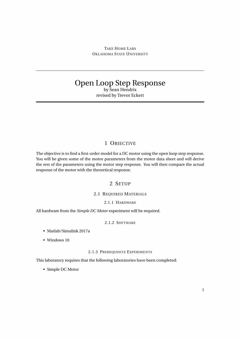
58. Double-click on the To Workspace block and type velocity in the box labeled “Variablename:" and then click OK.

11

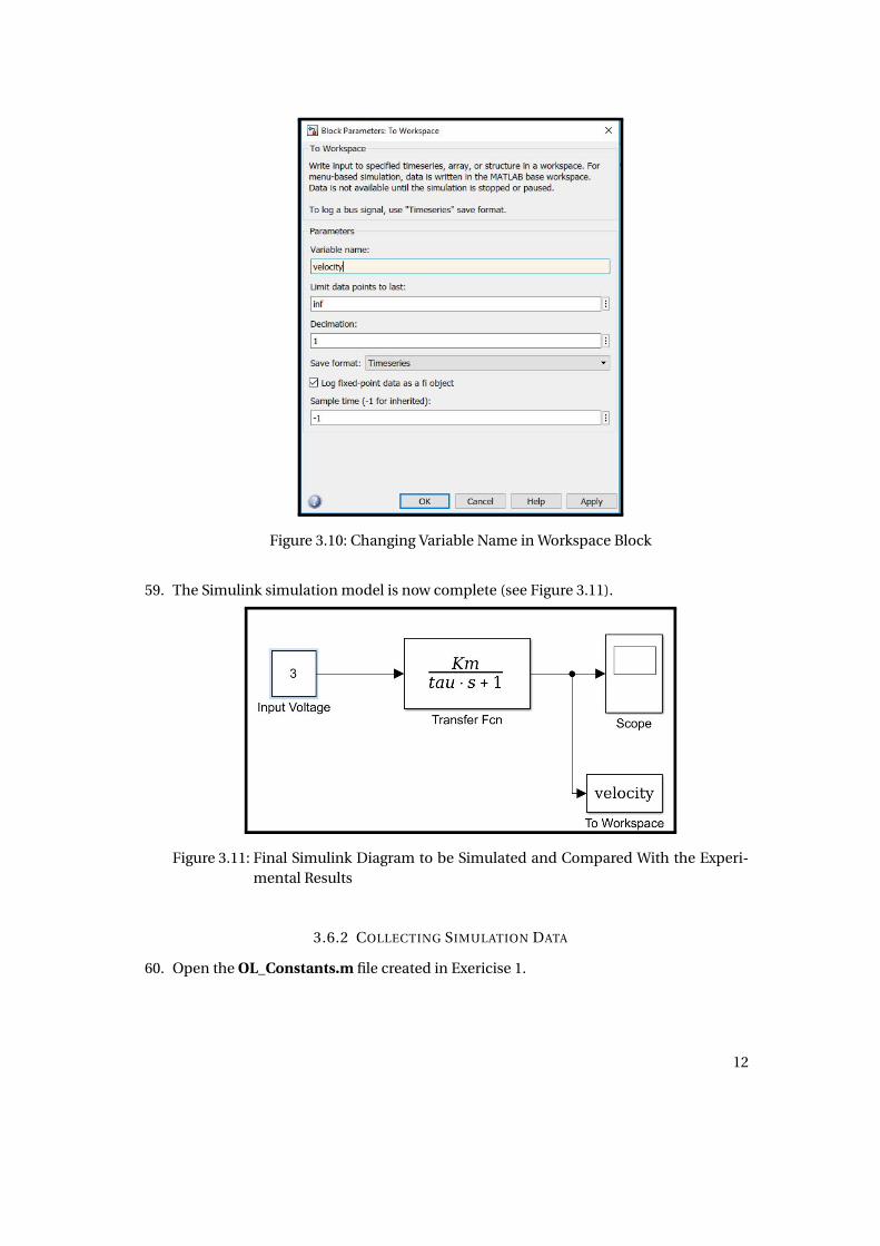
Figure 3.10: Changing Variable Name in Workspace Block

59. The Simulink simulation model is now complete (see Figure 3.11).

Figure 3.11: Final Simulink Diagram to be Simulated and Compared With the Experi-mental Results

3.6.2 COLLECTING SIMULATION DATA

60. Open the OL_Constants.m file created in Exericise 1.

12

61. Add the lines of code found in Figure 3.12 to the bottom of the m-file.

Figure 3.12: Add These Two Lines to Code

62. Replace each 0 value in the OL_Constants.m file (shown in Figure 3.12) with the valuesyou found for Km and τm in steps 41 and 42.

63. Save the file and then press the “Run" button at the top of the page. Navigate to the“MATLAB 2017a" home page. Under “Workspace" on the right-hand side of the page,all of the variables from “OL_Constants.m" should be listed below.

NOTE: if any variables created in the “Setting Up Matlab File" section are not listed un-der “Workspace," simply add the missing variables to the bottom of the OL_Constants.mfile and click Save once more. If any variables are missing from the OL_Constants.mfile, the “OL_Simulation.slx" file will not run correctly.

64. Open OL_Simulation.slx. Click the Run button at the top of the page.

65. Once the model has finished running, double-click on the Scope block. Click the Au-

toscale button .

NOTE: Observe the plot; does the response look similar to the response found in step33? If not, check the Km and τm values you found in steps 41 and 42. For now, theexact Km and τm values do not matter, just the general shape of the plot (which shouldbe increasing until it reaches a steady state value, where it stays constant, as in thetheoretical plot you made in Exercise 3).

66. Navigate back to the “MATLAB 2017a" home page. Under “Workspace" a new vari-able velocity should now be available. Right click on velocity and click “Save As..."Navigate to the folder in which you have saved this project, name the “File name:" as

CLSR_1.mat, and click Save at the bottom of the page.

3.6.3 EXPERIMENTAL VS. SIMULATION COMPARISON MATLAB FILE

67. Open the OL_Plot.m file you created in steps 38 - 40.

68. Copy and paste the text from Listing 2 to the bottom of OL_Plot.m. Click Save .

13

Listing 2: Code for Plotting Simulation Results (Added to OL_Plot.m)

%Load the simulated data and store into a variable

Sim_dat = load('CLSR_1.mat');

T1 = Sim_dat.velocity.Time;

Sim_dat = Sim_dat.velocity.Data;

%Plot the Simulated Data with Respect to Time

hold on;

plot(T1,Sim_dat,'Color', 'k', 'LineWidth', 2);

legend('Experimental', 'Simulation', 'Location', 'northwest');

69. Click Run at the top of the page.

70. Compare the responses of the simulation with the experimental data. Does the simu-lated response match the experimental response? Describe the similarities and differ-ences. Write down the current value for Km and τm on a piece of paper to keep track ofthem.

71. What would cause the differences between the responses?

72. If the plots look different, change the values for Km and τm to match the simulationwith the experimental open loop step response. After finding the new values, changethe Km and τm values in the OL_Constants.m file. After changing the OL_Constants.mfile, follow steps 60 - 69 once more. If the simulated and experimental open loop stepresponses look almost the same, continue to the next step.

73. How much (if any) did the new values for Km and tau change from your original values?For the new values of Km and τm , repeat step 45. How much did the values for J and βchange?

74. Finally, compute the pole of your system based on the transfer function you have de-rived.

4 TABLE OF DISCUSSIONS AND QUESTIONS

Before you turn in your report for this experiment, make sure that you have answered all ofthe questions that have been posed. It is important that your answers be expansive and thatthey demonstrate that you were mentally engaged in the experiment. Below is a recap of theimportant questions and the number of the step where each question was embedded.

14

steps Discussion/Question7 Solve for G1,G2,G3,G4

8 Find Ω(s)E(s)

9 Arrange in the form Kmτm s+1

10 Derive and plot response of ω(t )11 How does Km and τm affect the step response?12 Plot of pole along with description.41 Comparison of angular velocity vs. time of theoretical and experimental41 Calculate time constant τm

42 Calculate the DC gain Km

43 Finding first order transfer function with calculated experimental values44 How does the theoretical transfer function relate to the experimental transfer function?44 Find expressions for Km and τm in terms of Kt ,Kb , J ,β, and Ra

45 Calculate β and J46 Explanation of why the results may not be consistent65 Does the response look similar?70 Comparison of experimental and simulated response71 What could cause the differences between the responses72 Final plots73 Changes from initial to final values of Km ,τm ,β, and J

5 CONCLUSION

This experiment provided an analysis of the open loop step response of a DC motor. Theoret-ical, experimental and simulated responses were generated and compared. This experimentutilized the Simple DC Motorand Sampling and Data Acquisition experiments.

15