open inflation in the landscape misao sasaki (yitp, kyoto university) in collaboration with daisuke...
TRANSCRIPT

Open Inflation in the Landscape
Misao Sasaki(YITP, Kyoto University)
in collaboration withDaisuke Yamauchi (now at ICRR, U Tokyo)
andAndrei Linde, Atsushi Naruko, Takahiro Tanaka
Takehara workshop June 6-8, 2011
arXiv:1105.2674 [hep-th]

2
1. String theory landscape
There are ~ 10500 vacua in string theory
• vacuum energy v may be positive or negative
• some of them have v <<P4
• typical energy scale ~ P4
Lerche, Lust & Schellekens (’87), Bousso & Pochinski (’00), Susskind, Douglas, KKLT (’03), ...
which?

3 A universe jumps around in the landscape by quantum tunneling
• it can go up to a vacuum with larger v
• if it tunnels to a vacuum with negative v , it collapses within t ~ MP/|v|1/2.
• so we may focus on vacua with positive v: dS vacua
0
v
Sato, MS, Kodama & Maeda (’81)

4
2. Anthropic landscape
Susskind (‘03)
Not all of dS vacua are habitable.
“anthropic” landscape
• v,f must not be larger than this value in order to account for the formation of stars and galaxies.
A universe jumps around in the landscape and settles down to a final vacuum with v,f ~ MP
2H02 ~(10-3eV)4.
Just before it has arrived the final vacuum, it must have gone through an era of (slow-roll) inflation and reheating, to create “matter and radiation.”

5
Most plausible state of the universe before inflation is a de Sitter vacuum with v ~ MP
4.
false vacuum decay via O(4) symmetric (CDL) instanton
inside bubble is an open universe
Coleman & De Luccia (‘80)4 3,1( ) ( )O O

6
Anthropic principle suggests that # of e-folds of inflation inside the bubble should be ~ 50 – 60 : just enough to make the universe habitable.
Garriga, Tanaka & Vilenkin (‘98), Freivogel et al. (‘04)
Nevertheless, the universe may be slightly open:2 3
01 10 ~10
revisit open inflation!
Natural outcome would be a universe with 0 <<1.
• “empty” universe: no matter, no life
Observational data excluded open universe with 0 <1.
may be confirmed by Planck+BAOColombo et al. (‘09)

7
3. Open inflation in the landscape
• tunneling to a potential maximum ~ stochastic inflation
Simplest polynomial potential = Hawking-Moss model
Hawking & Moss (‘82)
2 3 4
22 3 4m
V • 4 potential:
Starobinsky (‘84)
– constraints from scalar-type perturbations –
2V H
slow-roll inflationHM transition
• too large fluctuations of unless # of e-folds >> 60 Linde (‘95)

8
• If inflation is short, too large perturbations from supercurvature mode of
2 2~ F R
sc
H H
? HF : Hubble at false vacuum
HR : Hubble after fv decay
MS & Tanaka (‘96)
0(3)
2 2 2| |; | | ( , )sc K p mp p K p K Y r l
Two- (multi-)field model: “quasi-open inflation”
• a “heavy” field undergoes false vacuum decay
• another “light” field starts rolling after fv decay
~ perhaps naturally/easily realized in the landscape
2
22,
mV V
Linde, Linde & Mezhlumian (‘95)
604
2
~N
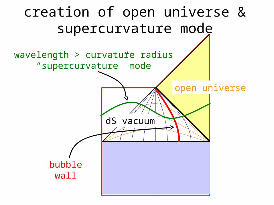
creation of open universe & supercurvature mode
bubble wall
open universe
dS vacuum
wavelength > curvature radius“supercurvature” mode
10
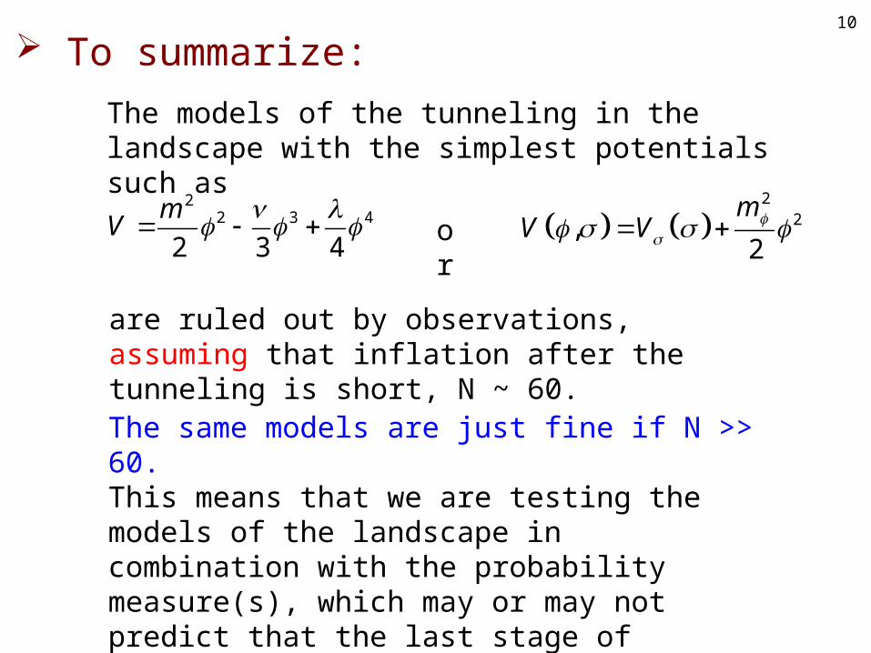
To summarize:
2
22,
mV V
The models of the tunneling in the landscape with the simplest potentials such as
2 3 4
22 3 4m
V or
are ruled out by observations, assuming that inflation after the tunneling is short, N ~ 60.
The same models are just fine if N >> 60.This means that we are testing the models of the landscape in combination with the probability measure(s), which may or may not predict that the last stage of inflation is short.

11 Single field model
• if fv ~ MP4, the universe will most likely tunnel to
a point where the energy scale is still very high unless potential is fine-tuned.
2FH
F
FV decay
rapid rollslow roll inflation
rapid-roll stage will follow right after tunneling.
• perhaps no strong effect on scalar-type pert’s:2
2~C
H
R &suppressed by at rapid-roll phase
1/ &
need detailedanalysis
∙∙∙ future issue
Linde, MS & Tanaka (’99)

12
but tensor perturbations may not be suppressed at all.
?~TT
P
Hh
M
Tensor perturbations and
their effect on CMB
Memory of HF (Hubble rate in the false vacuum) may remain in the perturbation on the curvature scale

13
4. Single field model- evolution after tunneling -
2FH
F
Right after tunneling, expansion is dominated by curvature:
,
4
Va t t
&
rapid-roll phase
2 1* */V t H &
: slow-roll parameter1
2
3
22( ) ( ),V
VH
V
1
3
2
2
aa a
&
curvature dominant phase
kinetic energy grows until
at

14
2FH
F
21
2VV
3
2
2
2
lnln /
dd a V
&&
1 1* * */~t H H
rapid-roll phase
2 1* */V t H & at
starts to decay at
21 1
3 2
2
2
aV
a a
& &
1,* ~ for
1 1* * */t H H =
1,* =for
V dominates (curvaturedominance ends) at
no rapid-roll phase. slow-roll inflation starts at
1*~t H
rapid-roll continues until
- continued
tracking is realized during rapid-roll phase 12 2/V a &
1 =

15 exponential potential model
exp 2V
2 2 2* * *exp 2R RV H H H
* 1
Log
10[r
/H*2
]
Log10[a(t) H*]
* 0.1
* 0.5
2* 10
4* 10
potential
kinetic term
curvature term
added to realizeslow-roll inflation
/V V const. const.
2 2* RH H?

16
VgRgL2
1
2
1
5. Tensor perturbations
some technical details...
2 2 2 2 2 2
2 2 2 2 2
( ) sin
( ) sin
E E E E E
C E E E E
ds dt a t dr r d
a d dr r d
• CDL instanton
( )E E
E
E
Er
bubblewall
• action

17
• analytic continuation to Lorentzian space (through rE=/2)
2,C E C Er i r
C-region: ~ outside the bubble
2 2 2 2 2 2( ) coshC C C C Cds a d dr r d
=const.
r =const.
Bubblewall
r C =0
R-region: inside the bubble
2 2, ,R C R C R Cr r i i a ia
2 2 2 2 2 2( ) sinhR R R R Rds a d dr r d
Euclidean vacuum C-region R-region
C=+ 8C=- 8
R
Ctime
time

18
2 (( ) , )( )TTij C p
p mij CC YX rh a l
2 1 0; 12
22 ( )C
pC C C
ad dp X K
d a d
2 pp
C
da X aw
d
;2
22 ( ) p p
T CC
dU w p w
d
2
2
2
2 2
( ) ( )
( ) ( )
T C C
C C C
U
a t t
&
• tensor mode function Euclidean vacuum
Yij: regular at rc=0
new variable wp :
UT
C
bubblewall
Cipe
Cipe Cipe
2 21

19
analytic continuation from C-region to R-region(=open univ.)
/ / 22C C R Rip ip ip ipp p p pC Rw e e w e ee e
2C R C i
• there will be time evolution of wp in R-region:
effect of wall
2 1 0 ; 2
22 ( ) R
pR R R
ad dp X
d d a
H H
R epoch of bubble nucleation:
0 ; 2
22 2
2 ( ) ( )pT R T R
R
dU p w U
d
or
final amplitude of Xp depends both on the effect of wall & on the evolution after tunneling
2
1 p TTp
dX aw h
a d

20
high freq continuum + low freq resonance
wall fluctuation mode1p 0~p
2
2 C Cs d
Effect of tunneling/bubble wall on
s ~ ∞
s ~0.1 s ~0.02
s ~1
s ~0.7
; 211~ C
P
Ss S dt
M V
&
scale-invariant
2( )T pP p X
wall tension

21
rapid-roll phase (* -)dependence of PT(p)
<<1: usual slow roll
~1: small p modes rememberH at false vacuum
>>1: No memory of H at false vacuum

22
6. CMB anisotropy
ℓ
~1: small ℓ modes remember initial Hubble
0(1 ) l• scales as at small ℓ, scale-invariant at large ℓ
<<1: the same as usual slow roll inflation
>>1: No memory of initial Hubble
1* ~ small ℓ modes enhanced for

23
• CMB anisotropy due to wall fluctuation (W-)mode
0
1(( )) ( );W W TWC P P dpC C pC P
s
l ll
%
01( )WC l
l% affect only
low ℓscale-invariant part
ℓ=22*2
2
/CH s
l
*s = 10-2
s = 10-5
s = 10-4
s = 10-3 W-modedominates
ℓ=2
MS, Tanaka & Yakushige (’97)

24
7. Summary Open inflation has attracted renewed interest in the context of string theory landscape
Landscape is already constrained by observations
anthropic principle + landscape 1-0 ~ 10-2 – 10-3
• simple polynomial potentials a2 – b3 + c4 lead to HM-transition, and are ruled out
• simple 2-field models, naturally realized in string theory, are ruled out
due to large scalar-type perturbations on curvature scale
If inflation after tunneling is short (N ~ 60):

25 Tensor perturbations may also constrain the landscape
“single-field models”
• it seems difficult to implement models with short slow-roll inflation right after tunneling in the string landscape.
• there will be a rapid-roll phase after tunneling.2
11
2 ~VV
right after tunneling
• unless>>1, the memory of pre-tunneling stage persists in the IR part of the tensor spectrum
due to either wall fluctuation mode or evolution during rapid-roll phase
We are already testing the landscape!
0(1 ) llarge CMB anisotropy at small ℓ