onstitutive modeling and mechanical behavior … · 2019-07-14 · constitutive modeling and...

Vieira, A.C., Guedes, R.M., Tita, V., “Constitutive modeling and mechanical behavior prediction of biodegradable polymers

during degradation.” In: “Biodegradable Polymers. Volume 1: Advancement in Biodegradation Study and Applications”,

Nova Publisher, 2015, p.31-75, ISBN 978-1-63483-632-6

Chapter

CONSTITUTIVE MODELING AND MECHANICAL BEHAVIOR PREDICTION OF BIODEGRADABLE

POLYMERS DURING DEGRADATION

André C. Vieira1, Rui M. Guedes2,3, Volnei Tita1 1Aeronautical Engineering Department, São Carlos School of Engineering,

University of São Paulo, São Carlos, São Paulo, Brazil 2Mechanical Engineering Department, Faculty of Engineering of University of Porto,

Porto, Portugal 3Porto Biomechanics Laboratory, University of Porto, , Porto, Portugal

ABSTRACT A large range of biodegradable polymers has been used to produce implantable medical devices, such as suture fibers, fixation screws and soft tissue engineering devices. Apart from biological compatibility, these devices should also be functional compatible and perform adequate mechanical temporary support during the healing process. The mechanical behavior of biodegradable polymers is known to be rate dependent and to exhibit hysteresis upon cyclic loading. On the other hand, ductility, toughness and strength of the material decay during hydrolytic degradation. Continuum based mechanical models can be used as dimensioning tools for biodegradable polymeric devices, since they enable to predict its mechanical behavior in a complex load and environment scenario, during the hydrolytic degradation process. The existing models can be divided into two categories: the time-dependent models and the time-independent models. Linear elastic or non-linear elastic models, such as elasto-plastic or hyperelastic models, can simulate the time-independent response, which corresponds to the relaxed configuration and represent the relaxed state. However, these approaches neglect the time-dependent mechanical behavior. To consider time dependency, dissipative elements must be used in the model formulation. A revision of the three-dimensional constitutive models generally used for polymers is presented in this chapter. These models are based on the concept of networks, combining elastic, sliding and dissipative elements, in order to simulate the time-dependent mechanical behavior, although neglecting changes in the properties of the material during hydrolytic degradation process. Thus, some of these models were recently adapted to address the hydrolytic degradation process. A common method consists on becoming some of the material model parameters dependent on a scalar variable, which expresses the hydrolytic damage.Furthermore, the advantages and limitations of the models are discussed, based on the correlation between predictions and experimental results of a blend of polylactic acid and polycaprolactone (PLA-PCL), which include monotonic tensile tests at different strain rates and quasi-static cyclic unloading-reloading.

André C. Vieira, Rui M. Guedes, Volnei Tita 2

Keywords: constitutive models, mechanical behavior, biodegradable polymers, hydrolytic degradation

INTRODUCTION Biodegradable polymers can be classified as either naturally derived polymers or

synthetic polymers. A large range of mechanical properties and degradation rates are possible among these polymers. However, the prediction of the mechanical behavior of these biodegradable devices is complex, because not only the mechanical properties evolve during degradation, but also these biodegradable polymers, in many situations, cannot be modeled using simple elastic constitutive equations. Due to the nonlinear nature of the stress vs. strain relation, the classical linear elastic model is not valid for simulation under large strains. Current designs of biodegradable devices are carried out by considering elastic or elastoplastic behavior and neglect any changing on the mechanical behavior of the device with degradation (Moore et al., 2010). For many biomedical applications, the biodegradable polymeric structures are submitted to cyclic loading above the elastic limit. Hence, they are prone to accumulate plastic strain at each cycle, which may lead to laxity and consequent failure. For instance, Grabow et al. (2007) showed that significant creep of polylactides under a constant load leads to strain accumulation and collapse.

Concomitantly to its nonlinear nature, the mechanical behavior of polymeric materials is also temperature and strain rate dependent (Bardenhagen et al., 1997). However, due to isothermal host environment, when the implantable devices are in service, temperature dependence will be neglected in this chapter. Moreover, under low strain rates, the mechanical behavior is viscous and, under high strain rates, it becomes brittle elastic (Bardenhagen et al., 1997). Thus, the polymeric mechanical behavior should be modeled by different constitutive laws, considering the strain rate range of interest (Ferry, 1980, Ward, 1979). For example, Soares (2008) and Grabow et al. (2007) confirmed the non linear viscoelastic characteristics of PLA. The mechanical behavior of biodegradable polymers is also known to exhibit hysteresis, i.e. energy dissipation in form of heat upon cyclic loading, as shown by Vieira et al. (2013) for PLA-PCL. Therefore, time-dependent constitutive models are required to simulate such phenomena.

As observed in polymers, it is known that the stress in a biodegradable polymer will relax towards an equilibrium state after being subjected to a strain-step (Miller and Williams, 1984). This relaxed state has been simulated by linear elastic, elasto-plastic or hyperelastic models, but disregarding the rate dependency effect. Moreover, the response of an elastic or hyperelastic material model implies that the loading and unloading paths coincide. Mechanical properties of biodegradable polymers are commonly assessed within the scope of linearized elasticity, despite the large strains, which are observed before material fracture. Thus, inelastic or hyperelastic models are required to simulate such strain range. Hence, considering the response of biodegradable polymers, classical models such as the neo-Hookean and Mooney-Rivlin models, usually applied for incompressible hyperelastic materials, have been used to predict mechanical behavior until rupture of non-degraded PLA (Garlotta, 2001, Lunt, 1998) under quasi-static monotonic loading. A single-order, isotropic Ogden material hyperelastic model was also used (Krynauw et al., 2011) to simulate the mechanical behavior evolution during degradation of a polyester-urethane scaffold. However, those approaches neglect changes in the properties of the material during degradation process.

Constitutive modeling and mechanical behavior prediction of biodegradable polymers during degradation

3

In the case of elasto-plastic models, after unloading phase, the material returns to a relaxed equilibrium sate, which includes inelastic strain. Since these models include at least one sliding element in its formulation, the loading and unloading paths do not coincide. Although, those models neglect the time-dependent mechanical behavior, they can simulate the time-independent response, which corresponds to the relaxed configuration.

To consider time dependency, dissipative elements represented by time inhomogeneous relations must be used in the model formulation. The simplest viscoelastic models consider a linear combination of springs (using the Hooke’s law) and dashpots (using Newtonian damper with linear viscosity). More complex variants of these simple models are based on the same concept of networks, combining elastic, sliding and dissipative elements, in order to simulate the equilibrium response of the material and the time-dependent deviation from equilibrium relaxed configuration.

However, those models are only able to simulate the initial mechanical behavior of polymers, neglecting changes in the properties of the material during the hydrolytic degradation process. It is possible to find only few scientific contributions in the literature (Khan and El-Sayed, 2013, Muliana and Rajagopal, 2012, Soares, 2008; Soares et al., 2010, Vieira et al. 2014) about the simulation of the mechanical behavior of biodegradable polymer during the hydrolytic degradation process. Therefore, the aim of this chapter is to explain a methodology to adapt different constitutive models in order to simulate the mechanical behavior during the hydrolytic degradation process. The concept behind this type of approach is to change the material model parameters as function of a scalar field, which represents the hydrolytic degradation and the correspondent chemical damage, inducing the changes of the mechanical behavior of the biodegradable materials. Hence, in the next section, there is a presentation about biodegradation process, namely describing the physical-chemical mechanisms and a simple way to model the degradation process based on the random scission assumption. Furthermore, the hydrolytic damage is defined and a failure criterion is established for biodegradable materials as function of degradation time. Then, after that, there is a brief review of some constitutive models generally used to simulate the mechanical behavior of conventional polymers under hydrolytic degradation by using the proposed methodology. Some examples are shown, and the potential of each type of constitutive model are discussed and compared for different loading situations.

BIODEGRADATION PROCESS

All biodegradable polymers contain hydrolysable or oxydable bonds. This makes the

material sensitive to moisture, heat, light and also mechanical stress. These different types of polymer degradation (photo, thermal, mechanical and chemical degradation) can be present alone or combined, working synergistically to the degradation. Usually, the most important degradation mechanism of biodegradable polymers is chemical degradation via hydrolysis or enzyme-catalyzed hydrolysis (Göpferich, 1996). Hydrolysis rate is affected by the temperature or mechanical stress, molecular structure, ester group density as well as by the degradation media used. The crystalline degree may be a crucial factor, since enzymes attack mainly the amorphous domains of a polymer. The most important factor is its chemical structure and the occurrence of specific bonds along its chains. Like those in groups of esters, amides, etc., which might be susceptible to hydrolysis when exposed to water (Nikolic et al., 2003; Herzog et al., 2006).


Another important distinction must be made between erosion and degradation. Both are irreversible processes. The erosion process can be described by phenomenological diffusion-reaction mechanisms. An aqueous media diffuses into the polymeric material while oligomeric products diffuse outwards to be then bio-assimilated by the host environment. Then, there is material erosion with correspondent mass loss. Hence, the degree of erosion is estimated from the mass loss. On the other hand, degradation refers to mechanical damage and depends on hydrolysis. Within the polymeric matrix, hydrolytic reactions take place, mediated by water and/or enzymes. Polymer degradation is the first step of the erosion phenomenon and can be estimated by measuring the evolution of molecular weight, by size exclusion chromatography (SEC) or gel permeation chromatography (GPC), or the tensile strength evolution (by universal tensile testing). Therefore, the hydrolytic degradation process is included on the erosion process. The complete erosion of the polymer is known to take substantially longer than the complete loss of tensile strength. During this first phase, aqueous solution penetrates the polymer, followed by hydrolytic degradation, converting these very long polymer chains into shorter water-soluble fragments.

Physical-Chemical mechanisms and modeling Hydrolysis has been traditionally modeled by using a first order kinetics equation based

on the random scission kinetic mechanism of hydrolysis, according to the Michaelis–Menten scheme (Bellenger et al., 1995). In the case of aliphatic polyesters, such as PLA, each polymer molecule, with its own carboxylic and alcohol end groups, is broken in two. This occurs randomly in the middle at a given ester group. So, the number of carboxylic end groups will increase with degradation time, while the molecules are being split by hydrolysis. The following first-order equation describes the hydrolytic process (Farrar and Gilson, 2002), in terms of the rate of formation of carboxyl end groups:

uckewcdt

dc == Eq. 1

where e, c and w are the concentrations of ester groups, carboxyl groups and water in the

polymer, respectively. k is the hydrolysis rate constant and t is the degradation time. u is the hydrolytic degradation rate of the material, which can be determined by measuring strength or molecular weight evolution during hydrolytic degradation (see Vieira et al., 2011a). Since the concentration of carboxyl end groups is given by c=1/Mn, where Mn is the number-average molecular weight of the polymer, the evolution of the number-average molecular weight is given, after integration, by:

ut

nn eMM0t

−= Eq. 2

where Mnt is the number-average molecular weight of the polymer at degradation time t

and Mn0 is the initial (non-degraded) value. Degradation rate u is affected by many factors that can vary along the volume or during degradation. For example, temperature will increase the hydrolysis rate constant k, which is associated to the probability of bond scissions, due to excitement of the molecules. In the case of implantable devices, the temperature is kept constant as in the human body, i.e. at the homeostatic value around 37ºC.

The influence of the mechanical environment in the degradation rate has been also reported at literature (Chu, 1985; Miller and William, 1984). Similarly to temperature, stress applied during the degradation process also increases the probability of bond scissions, and


5

consequently increases the degradation reaction rate constant k. Some studies on rubbery polymers include the effect of micro structural changes in the polymer’s macromolecules, crosslinks and entanglements (Huntley et al., 1996; Rajagopal et al., 2007; Rajagopal and Wineman, 1992; Shaw et al., 2005; Smeulders and Govindjee, 1999; Wineman and Min, 2002). In those approaches, not specifically related to hydrolytic degradation, micro structural changes depend on state variables, which locally measure chain stretches. Later, other researchers (Khan and El-Sayed, 2013; Muliana and Rajagopal; 2012, Soares, 2008; Soares et al., 2010) developed their methodologies based on those works previously published, in order to introduce the influence of the strain field in the hydrolytic degradation.

Concerning the degradation dependence, some authors reported that the degradation rate of PLA and blends of PLA-PCL was significantly affected by some enzymes (Gan et al., 1999; Williams, 1981). The pH of the aqueous media also affects the degradation reaction rate constant k (Tsuji and Ikada, 1998; Tsuji and Ikada, 2000; Tsuji and Nakahara, 2001). Again, in the case of implantable device, pH can be considered constant, because, pH is kept at a homeostatic value in the human body. Hence, in many cases, it can be assumed that the hydrolysis rate k is constant over time due to constant temperature, load (i.e. constant stress field during degradation) and degradation media.

In the particular case of biodegradable polymers, water diffusion is very fast compared to water-mediated hydrolysis. Therefore, water can be assumed, in many cases, to be spread out uniformly in the sample volume (i.e. no diffusion control) from the beginning of erosion process, and hydrolysis promotes homogeneous bulk erosion (Li et al., 1990). This assumption is reasonable for small thickness or porous devices. Hence, w can also be assumed constant from the beginning along the volume. Otherwise, the water concentration along the volume and during time can be computed using the Fick’s Second Law. In this early stage of erosion, when mechanical strength reduces significantly, the concentration of ester groups e located at the backbone chains is nearly constant. Despite of the scissions, which occur randomly in the ester groups, the macromolecules remain large (Göpferich and Langer, 1993). Considering all this assumptions, the degradation rate, u=kwe, may be considered constant during the whole degradation process. In some cases, as explained previously, these assumptions are not valid, mainly because of heterogeneous diffusion of water, or due to the presence of a complex three-dimensional stress field, which evolves during the degradation process.

Hydrolytic damage and failure criteria It is well known that the mechanical behavior will evolve during time, due to hydrolytic

chain scission in the polymeric macromolecules. In figure 1a is shown the mechanical response to uniaxial monotonic tensile tests until rupture for PLA-PCL fibers during hydrolytic degradation The reduction of molecular weight is linked to this evolution in mechanical response of biodegradable polymers. It has been shown by Vieira et al. (2011a) that the fracture strength σ during degradation can be predicted by the following equation:

kwet

0ut

0t ee −− == σσσ Eq. 3

where σt is the strength of the polymer at degradation time t and σ0 is the initial (non-

degraded) strength. The evolution of fracture strength, according to equation 3, is similar to the evolution of the number-average molecular weight of the polymer (see figure 1b) in accordance to equation 2. In a semi logarithmic representation of normalized strength or number-average molecular weight versus degradation time, the degradation rate u


corresponds to the slope of the linear fit. Further details of this degradation study can be found in Vieira et al. (2011a).

Figure 1 – a) Monotonic tensile test results during hydrolytic degradation of PLA-PCL fibers;

b) Evolution of the normalized strength and molecular weight during degradation of PLA-PCL fibers (adapted from Vieira et al., 2011a)

The hydrolytic damage was defined by Vieira et al. (2011a), according to equation:

ut

n

n

0

th e1

M

M11d

o

t −−=−=−=σσ

Eq. 4

From equation 4, it is possible to relate hydrolytic damage with strength and molecular

weight. Hence, hydrolytic damage is a local internal variable since the degradation rate can vary locally in the case of heterogeneous degradation. In order to simulate the evolution of the mechanical behavior of biodegradable polymers, the constitutive models must be adapted accordingly to hydrolytic damage dh.

It is possible to find only few scientific contributions in the literature about modeling of the mechanical behavior of biodegradable polymers during the hydrolytic degradation process. Those approaches are based on hyperelastic models (Soares et al., 2010; Vieira et al., 2011a), or on quasi-linear viscoelastic models (Muliana and Rajagopal, 2012), or on viscoplastic models (Khan and El-Sayed, 2012; Vieira et al., 2014). These approaches enable the modeling of biodegradable structures during degradation by assuming that the constitutive model parameters have been changed according to hydrolytic damage. In Muliana and Rajagopal (2012), hydrolytic damage is assumed to be dependent on the deviatoric strain tensor and the concentration of water.

CONSTITUTIVE MODELS FOR POLYMERS WITH BIODEGRADATION

PROCESS


7

Continuum mechanics is always the base for the generalization of constitutive models to three-dimensional approach. Hence, for the sake of completeness, there is a brief review and definitions on finite continuum mechanics in the Appendix and more details can be found in Malvern (1969). A constitutive model for a mechanical analysis is a relationship between the response of a body (for example, strain state) and the stress state due to the forces acting on the body, which can include the environmental effects. The actual models can be divided into two main categories: the time-independent and the time-dependent models.

Linear elastic constitutive model In uniaxial models, the applied stress, considered uniform along the surface perpendicular

to the applied load, is the ratio between the applied load and the initial surface area (nominal stress, i.e. Lagrange description), σ=F/A0, or alternatively the ratio between the applied load and the current surface area (true stress, i.e. Euler description), σ=F/A. In this case, the linear strain is defined by the ratio between elongation and the initial length, ε=(L- L0)/L0, and stretch is defined by the ratio between current length and the initial length, λ=1+ ε =L/L0. The uniaxial linear elastic model (the Hooke’s law) establishes a linear relation between stress and strain, σ= Eε, defined by a single material parameter E (Young modulus). This linear elastic rheological model is represented by a linear spring.

The generalization of the linear constitutive model to three-dimensional approach, according to a Largrange description, considering relation between the second Piola-Kirchhoff stress tensor S and the Lagrangian strain tensor E (see definitions in Appendix), is defined by an elastic stiffness fourth order tensor C:

klijklij ECS = Eq. 5

Alternatively, in the Euler description, considering the relation between the Cauchy stress

tensor T and the Eulerian strain tensor E* (see definitions in Appendix):

*kl

*ijklij ECT = Eq. 6

The relation between the two elastic stiffness tensors, in the Lagrange and Euler

descriptions, is:

nlmkpqkljqipnlmkpqkljqip*ijnm J

1RRCRRFFCFFC ≈= Eq. 7

where the Jacobian J, the deformation gradient F and the rotation tensor R are defined in Appendix.

Due to the isotropic nature of polymers, only isotropic models will be discussed in this chapter. Hence, considering an isotropic material, only two independent material parameters are needed to define all the components of the elastic stiffness fourth order tensor. Most commonly, the generic three-dimensional linear constitutive model, for isotropic materials, is presented in the form (according to Lagrange and Euler description respectively):


−+

+= ijkkijij 211

E δυ

υυ

EES Eq. 8

−+

+= ij

*kk

*ijij 211

E δυ

υυ

EET Eq. 9

where the Young’s modulus E and the Poisson’s ratio υ are the two independent material

parameters. The Kronecker delta function δij is defined in Appendix. If the stress tensor is known, it is possible to compute the strain tensor using the inverse relation:

klijklij SSE = Eq. 10

kl*ijkl

*ij TSE = Eq. 11

where ijklS and *ijklS are elastic compliance fourth order tensors in the Lagrange and

Euler descriptions, respectively. Therefore, for isotropic materials, the constitutive relation may have the form:

ijkkijij EE

1 δυυSSE −+= Eq. 12

The fourth order stiffness and compliance tensors, for isotropic materials, are hence

defined respectively:

( ) ( ) ( )( )( ) klijjlikjkil

klijjlikjkilijkl 211

E

12

E

δλδδδδδµ

δδυυ

υδδδδυ

++=

=−+

+++

=C Eq. 13

( ) klijjlikjkilijkl EE2

1 δδυδδδδυ −++=S Eq. 14

where the shear modulus, ( )υµ += 12/E , and the Lamé’s

constant, ( )( )υυυλ 211/E −+= , are other alternative material parameters commonly used

to characterize the elastic behavior of polymers. Another material parameter usually found in

the Hooke’s generalized model is bulk modulus, ( )υκ 213/E −= .

Linear elastic model is unable to capture yielding. Moreover, it is possible to see in figure 1a) that, in the linear region, the Young modulus E remains nearly unchanged during degradation. However, at large strains, the linear elastic model is able to fit reasonably well the experimental monotonic tensile test results. Another limitation of this model is that it is time-independent. Hence, it is unable to capture the mechanical behavior dependence on the strain rate, as can be seen in figure 2a for the monotonic tensile test at two different strain rates (15 and 500 mm/min), when both experimental results were used to calibrate the


9

parameters of the model by inverse analyses. It is also unable to capture hysteresis and plastic strain accumulation, since the unloading path is the same of the reloading path (see figure 2b). In this second case, unloading-reloading tensile tests results were used to calibrate the model parameters. On one hand, the linear elastic model predicts the same result independently from the strain rate (see figure 2a). On the other hand, the loading and unloading paths coincide in the same linear prediction. The calibration technique used to minimize the difference between the experimental results and the model predictions was the Nelder-Mead method.

Figure 2 –Experimental results of a) monotonic tensile test at two strain rates (500 and 15

mm/min) and b) cyclic tensile test of a biodegradable polymer (PLA-PCL), and prediction of linear elastic model.

Calibration of the model was done based on the monotonic tensile tests results (at 250

mm/min) at four degradation steps (0, 2, 4 and 8 weeks). Considering that the Poisson’s ratio υ remains unchanged (0.4) during degradation, the elastic modulus E was determined by calibration at each degradation step. Then estimated values were fitted by linear regression as function of the degradation damage d(t,u). In the figure 3, it is possible to observe that the elastic modulus E decreases nearly linear as function of the hydrolytic damage.

E = -793.12dh + 1489.4R² = 0.9407

1000

1100

1200

1300

1400

1500

1600

0.0 0.1 0.2 0.3 0.4 0.5 0.6

dh

Linear elastic

Figure 3 –Evolution of the elastic modulus E during hydrolytic degradation.

Based on this linear equation to estimate the elastic modulus E(d), the mechanical

behavior of the polymer was predicted. The results are shown in figure 4.

a) b)


Figure 4 – Experimental results of monotonic tensile test at 250 mm/min of PLA-PCL fiber,

and model results via linear elastic model, after 0, 2, 4 and 8 weeks of hydrolytic degradation.

Hyperelastic constitutive models Besides the linear elastic model, hyperelastic models can be used to model the relaxed

state. Polymeric materials are known by their non-linear mechanical behavior. Hyperelastic models are a class of constitutive relationships able to model nonlinear elasticity. Mechanical properties of hyperelastic materials are usually represented in terms of a strain energy density function W. Considering the one-dimensional representation of hyperelastic models, the constitutive relation is generically defined by:

εσ

d

dW= Eq. 15

where σ and ε are the stress and strain measured by the uniaxial tensile test, where W is

defined by:

( )∫= εεσ dW Eq. 16

and represents the area below the stress-strain curve. Hyperelastic models should have

the ability to reproduce the ‘S’ shaped response of rubber like materials (Chagnon et al., 2004).

A general polynomial form usually found for the strain energy density, assuming an incompressible mechanical behavior, is defined in terms of the strain invariants:


11

( ) ( ) ( )∑=

−−=N

0j,i

jiij 3II3IcII,IW Eq. 17

where λλ /2I 2 += is the first invariant and λλ 2/1II 2 += is the second invariant and cij are material parameters.

In the case of hyperelastic models, generalizing to the three-dimensional representation, W is a scalar function of the deformation gradient F. The rate of work done by stresses acting on a small material element with volume dV0 in the undeformed solid may be defined as:

0ijijij

ij

dVt

W

t

WW PF

F

Fɺɺ =

∂∂

∂∂=

∂∂= Eq. 18

Then, a generic form for a hyperelastic constitutive relation can be presented in terms of

the first Piola-Kirchhoff stress tensor P:

ijij

W

FP

∂∂= Eq. 19

or in terms of Cauchy stress tensor T:

kjikij

W

J

1

FFT

∂∂= Eq. 20

As referred previously for the one-dimensional model, this constitutive relation is usually

defined in terms of the invariants of the left Cauchy-Green deformation tensor B (see definition in Appendix). The first, second and third invariants are defined, respectively, as:

( ) 23

22

21kkijB trI λλλ ++=== BB Eq. 21

[ ] 21

23

23

22

22

21kiik

2BB I

2

1II λλλλλλ ++=−= BB Eq. 22

23

22

21

2kkB JIII λλλ=== B Eq. 23

where ��, � = 1, 2, 3 are the eigenvalues of F, and also known as principal stretches. The

formulas for the strain energy function are generally expressed in terms of principal stretches:

( ) ( ) ( ) ( )[ ]( ){ }∑=

−+++++=N

0k,j,i

k321

j2

j1

i3

j1

j3

i2

j3

j2

i1ijk3,2,1 6aW λλλλλλλλλλλλλλλ

Eq. 24


where ijka are material parameters, or in terms of the invariants of the Cauchy-Green

deformation tensors:

( ) ( ) ( ) ( )∑=

−−−=N

0k,j,i

kB

jB

iBijkBBB 3III3II3IcIII,II,IW Eq. 25

where ijkc are material parameters. Many elastomeric and polymeric materials are often

nearly incompressible. Hence, it is more convenient to use an alternative set of invariants of the deviatoric left Cauchy-Green tensor (i.e. neglecting the volumetric part of the strain tensor):

B3/2

B IJI −= Eq. 26

B3/4

B IIJII −= Eq. 27

Therefore, it is common to find the strain energy density function in the generic

polynomial form (Forni et al., 1999), in terms of this alternative set of invariants:

( ) ( ) ( ) ( )∑ ∑=

−+−−=N

0k,j,i

M

i

i2i

j

B

i

BijBB 1Jd3II3IcJ,II,IW Eq. 28

where cij are the material parameters related to distortion, whereas di are the material

parameters related to volume change. Note that for incompressible materials J is equal to “1”.

Particular cases of this general polynomial form, considering ( )J,II,IW BB , are:

- the Neo-Hookean model, where i=1, j=0 and N=M=1:

( ) ( ) ( )21B10BB 1Jd3IcJ,II,IW −+−= Eq. 29

Solving equation 20, the corresponding constitutive relation results in:

( ) ij1ijkkij3/510

ij 1Jd23

1

J

c2 δδ −+

−= BBT Eq. 30

- the Mooney-Rivlin model, where c00=0, c11=0, and N=1:

( ) ( ) ( ) ( )21B01B10BB 1Jd3IIc3IcJ,II,IW −+−+−= Eq. 31

The corresponding constitutive relation is:


13

[ ] ( ) ij1ijnkknkiikij2

kkijkk3/701

ijkkij3/510

ij

1Jd23

1

3

1

J

c2

3

1

J

c2

δδδ

δ

−+

+−−+

+

−=

BBBBBBB

BBT

Eq. 32

where in these cases 2d1=κ. The simplest hyperelastic model for elastomeric materials is

the Neo-Hookean model. It is a Gaussian statistical theory model, because the strain energy function was originally defined as:

( ) ( )32

Tn3I

2W 2

322

21B −++=−= λλλβµ

Eq. 33

where the shear modulus µ is a function of the chain density (n), Boltzmann’s constant

(β) and temperature (T). See Treloar (1975) for a more detailed description of Gaussian statistics and the corresponding assumptions. On the other hand, the Mooney-Rivlin model is an empirical model. Although it is one of the most favorite models, its disadvantage is that material parameters must be obtained by mechanical experiments since they are not physically consistent. Other sophisticated empirical models, variants of the generic polynomial forms, such as Odgen model or Yeoh model, can be found in literature.

A good constitutive model should represent the three-dimensional nature of the stress-stretch behavior using a minimal number of parameters to represent physically the deformation process. Ideally, the parameters should be obtainable from a small number of experiments, preferably only one (Arruda and Boyce, 1993b). In this sense, Yeoh model is an empirical simple model, applicable for a wider range of deformation and is able to predict the stress-strain behavior in different deformation modes (such as compression or shear) from data gained in one simple deformation mode (such as uniaxial extension)(Ghosh et al., 2003). Other physical models are based on chains networks described by Gaussian statistics or modified by the chain statistics to allow larger stretches than those afforded by the Gaussian statistics assumption. They incorporated these non-Gaussian chains into networks of three, four or an infinite number of chains (Wang and Guth, 1952; Flory and Rehner, 1943; Treloar, 1946). These models have in common two physically based parameters, the shear modulus (µ) and a chain locking stretch (λL) defined as the value of the chain stretch when the chain length reaches its fully extended state. However, these refereed models fail in the task of describing the response of an elastomeric material under different states of deformation without changing the model parameters (Arruda and Boyce, 1993b). The Arruda-Boyce model, also known as eight-chain model, is a sophisticated physical model able to predict the stress-strain behavior in different deformation modes from data gained in one simple deformation mode. It can be considered an extension of the Neo-Hookean model, which considers non-linear Langevin chain statistics when deriving the strain energy function. The strain energy is assumed equal to the sum of the strain energies of the individual chains randomly oriented in space, as defined below (Raoult et al., 2005):


( ) ( )

( ) ( ) ( ) ( )21

3

BL

2

BL

B

N

1i

21

ii

B2i2L

i

1Jd...27I1050

119I

20

13I

2

1

1Jd3Ic

W

−+

+−+−+−=

=−+−= ∑=

−

λλµ

λµ

Eq. 34

with the first five terms ci for the Taylor expansion of an inverse Langevin function are c1=1/2, c2=1/20, c3=11/1050, c4=19/7000, c5=519/673750. The corresponding constitutive relation is:

( ) ij1ijkkij4L

3/4kk

2L

3/2kk

3/5ij 1Jd23

1...

J525

33

J51

Jδδ

λλµ −+

−

+++= BB

BBT

Eq. 35 Although, hyperelastic models are non-linear they are unable to capture yielding.

However, at large strains, they are able to fit reasonably well the experimental monotonic tensile test results. Another limitation of these types of models is that they are not time-dependent. Hence, similarly to the linear elastic model, they are unable to simulate the mechanical behavior dependence on the strain rate, as can be seen in figure 5a for the monotonic tensile test at two different strain rates (15 and 500 mm/min), when both experimental results were used to calibrate the parameters of the model by inverse analyses. They are also unable to capture hysteresis and plastic strain accumulation, since the unloading path is the same of the reloading path (see figure 5b). In this second case, unloading-reloading tensile test results were used to calibrate the model parameters. The same calibration technique was used.


mm/min) and b) cyclic tensile test of a biodegradable polymer (PLA-PCL), and prediction via Arruda-Boyce model.

Calibration of the Arruda-Boyce model was done based on the monotonic tensile tests results (at 250 mm/min) at four degradation steps (0, 2, 4 and 8 weeks). Considering that the

a) b)


15

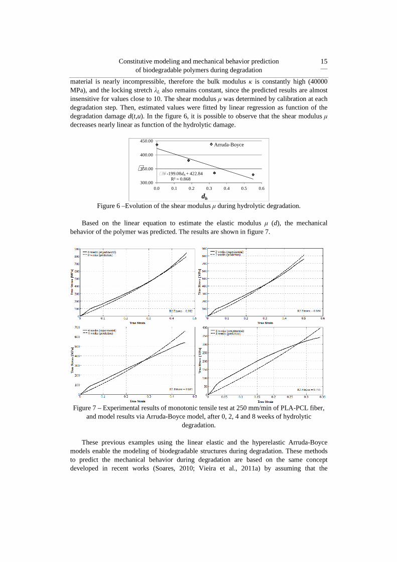
material is nearly incompressible, therefore the bulk modulus κ is constantly high (40000 MPa), and the locking stretch λL also remains constant, since the predicted results are almost insensitive for values close to 10. The shear modulus µ was determined by calibration at each degradation step. Then, estimated values were fitted by linear regression as function of the degradation damage d(t,u). In the figure 6, it is possible to observe that the shear modulus µ decreases nearly linear as function of the hydrolytic damage.

= -199.08dh + 422.84R² = 0.868

300.00

350.00

400.00

450.00

0.0 0.1 0.2 0.3 0.4 0.5 0.6

dh

Arruda-Boyce

Figure 6 –Evolution of the shear modulus µ during hydrolytic degradation.

Based on the linear equation to estimate the elastic modulus µ (d), the mechanical

behavior of the polymer was predicted. The results are shown in figure 7.


and model results via Arruda-Boyce model, after 0, 2, 4 and 8 weeks of hydrolytic degradation.

These previous examples using the linear elastic and the hyperelastic Arruda-Boyce

models enable the modeling of biodegradable structures during degradation. These methods to predict the mechanical behavior during degradation are based on the same concept developed in recent works (Soares, 2010; Vieira et al., 2011a) by assuming that the


constitutive model parameters have been changed according to hydrolytic damage. In these works other hyperelastic constitutive models, such as Neo-Hookean and Mooney-Rivlin, are used.

In another work (Vieira et al., 2011b), the Neo-Hookean hyperelastic model was implemented in ABAQUS through a User Material (UMAT) subroutine and PYTHON language. This script is run by ABAQUS and the degradation time is required as an input parameter data. The hydrolysis rate of the material u and the strength of the non-degraded material σ0 are initially set. Then the script calculates the hydrolytic damage dh according to equation 4 and the material strength σt, according to equation 3, was used in an implemented failure criterion in order to simulate a PLA-PCL fiber mechanical behavior until rupture in different stages of degradation, where is given the degradation time t. The script also calculates the material parameter c10 as a linear function of the hydrolytic damage dh. In Vieira et al. (2011b), the load, or the stress field, was assumed constant during hydrolytic degradation, since the specimens degraded in a stress free state.

In the work of Soares et al. (2010), the rate of degradation depends on the deformation gradient d(F) and implicitly on both location and time. They defined the deformation-

dependent reaction rate using the first and second invariants of the left Cauchy tensor, ijB ,

that is:

( ) ( ) ( )[ ]222 3311 −−−=

∂∂

BBd

h IIIdt

d

τ Eq. 36

where dτ is the characteristic time of degradation. As consequence, inhomogeneous

deformations, occurring in the body, can cause that some parts of it to degrade faster than others. However, these hyperelastic models neglect the time-dependent mechanical behavior. As seen before, they are unable to predict relaxation and creep.

Elastoplastic constitutive models Elastoplastic models are commonly used to simulate the mechanical behavior of metals,

including the yielding and hardening phenomena. In certain conditions, some features of the mechanical behavior of polymers can also be simulated using these types of models. One of the classical models described in literature is Saint-Venant plastic model, which represents a solid sliding over a surface with some friction (see figure 8). The yield stress is a material parameter, which represents the value above yielding, otherwise if this value is below, then there is no strain.


17

Figure 8 - Rheological representation of the perfectly plastic model

According to the Boltzmann superposition principle, elastic and sliding elements can be

combined in series or in parallel. Regarding this principle, each loading step produces independent contribution to total loading history and the total final deformation is the sum of each contribution. Thus, it is possible to model the elastic perfectly plastic model (Prandlt-Reuss model), represented in figure 9, where the elastic and sliding elements are combined in series.

Figure 9 - Rheological representation of the elastic perfectly plastic model

It is also possible to combine elastic and sliding elements in parallel (see figure 10),

adding the linear isotropic hardening into the perfectly plastic model. The material parameter H represents the hardening rate.

Figure 10 - Rheological representation of the linear isotropic plastic model Another classical example of a plastic model is the power law isotropic hardening,

represented in figure 11.


Figure 11- Rheological representation of the power law isotropic plastic model

To model the elastoplastic mechanical behavior of polymer and the permanent plastic strain εp accumulated after a load cycle, the bilinear elastoplastic model represented in figure 12 is also widely used. It results from the combination in series of linear isotropic plastic model and a linear elastic model.

Figure 12- Rheological representation of the bilinear isotropic elastoplastic model

In these one-dimensional models, total strain can be decomposed in an elastic part, recovered when the material is unloaded, and a plastic irreversible part, which remains after unloading:

pe εεε += Eq. 37

For the generalization of this decomposition, in the case of three-dimensional constitutive

elastoplastic models, the general strain increment is considered. According to a Lagrange description, this decomposition is defined as:

pij

eijij ddd EEE += Eq. 38


19

The linear constitutive relation for the elastic parcel results:

klijklij dd ECS = Eq. 39

A yield criterion must be established for the plastic part, to determine the critical stress

state required to cause permanent deformations in the polymer. The two most used criteria are the von-Mises and the Tresca, defined respectively by their yield surface:

( ) ( ) ( ) ( )[ ] y2

322

312

21pij 2

1,Tf σσσσσσσε −−+−+−= Eq. 40

( ) { } y323121pij ,,max,Tf σσσσσσσε −−−−= Eq. 41

Considering the Cauchy stress tensor, where σ1, σ2 e σ3 are their eigenvalues, the criteria

are defined so that the material deforms elastically when ( ) 0,Tf pij <ε , and plastically when

( ) 0,Tf pij =ε . Due to the yield criterion, ( ) 0,Tf pij =ε , which defines a surface in stress

space, it is referred to as a yield surface. These two yielding criterion may be plotted in a three-dimensional space, with the three principal stresses as axes (see figure 13).

Figure 13 – Yield surface according to Tresca and Von-Mises criteria

The axis of these prisms, according to each criterion, corresponds to a hydrostatic stress

sate, where σ1=σ2=σ3=σm=1/3(σ1+σ2+σ3). Hence, if the state of stress falls within the cylinder, the actuating stress is below yield level and the material shows elastic response. On the other hand, if the state of stress lies on the surface of the prism, the material yields and deforms plastically.

Alternatively, the von-Mises criterion can be expressed directly in terms of the stress tensor:

( ) yijijpij ''2

3,Tf σε −= TT Eq. 42


considering that the stress tensor can be decomposed into a volumetric stress tensor

related to volume changes during straining:

ijmijkkij 3

1'' δσδ == TT Eq. 43

and a deviatoric stress tensor related to distortions during straining:

ijkkijij 3

1' δTTT −= Eq. 44

This yield criterion is based mainly on the experimental observation for metals, where

hydrostatic stress (σ1=σ2=σ3=σm) can not cause yield. On other words, plastification phenomenon is assumed to be an isochoric process, regarding von-Mises criterion.

If the plastic deformation causes strain hardening to the material, the yield surface will change during plastic strain evolution. Then the yield stress, σy, determined from uniaxial monotonic tests, may increase during plastic strain evolution, due to hardening, when the polymer is reloaded. Hence, yield stress is a function of the plastic strain σy(εp). Among all the plastic constitutive models, the hardening law, which defines the evolution of the yield surface, must be established. The two most common approaches are the isotropic and the kinematic hardening models. In the case of the isotropic hardening model, the yield surface expands, but maintains the same shape. To get a suitable scalar measure of plastic strain, the accumulated plastic strain magnitude is defined:

∫= pij

pijp dd

3

2EEε Eq. 45

Then it is possible to establish the function σy(εp). The most common hardening function

are the perfectly plastic, the linear isotropic plastic and the power law isotropic plastic models, discussed above, and defined respectively as:

0yy σσ = Eq. 46

p0yy Hεσσ += Eq. 47

( ) m1

p0yy H εσσ += Eq. 48

where σy0 is the initial yield stress. An isotropic hardening law is generally not useful to

simulate the mechanical behavior of polymers, when these are subjected to cyclic loading around zero, as represented in figure 14. Isotropic models do not account for the Bauschinger’s effect, and so predicts that after a few cycles, the polymer will just harden until it shows elastic response.


21

Figure 14- Bauschinger’s effect prediction according to isotropic and kinematic hardening

models

The kinematic hardening law allows the yield surface to translate, without changing its shape. As the material is loaded in tension, the yield surface is displaced in the direction of increasing stress, thus it is possible to simulate the strain hardening. However, this softens the material in compression. Hence, the kinematic hardening models are able to simulate cyclic plastic deformation between tensile and compression. These two different yield surface evolutions during straining are graphically shown in figure 15.

Figure 15- Representation of yield surface changing during plastic strain evolution, according to: a) isotropic hardening model; b) kinematic hardening model

To consider this translation of the yield surface (without shape changes) during

hardening, the center of the yield surface is displaced to position αij in stress space. Hence, the von-Mises yield criterion needs to be modified as follows:

( ) ( )( ) yijijijijpij ''2

3,Tf σε −−−= αTαT Eq. 49

In this case, yield stress is constant, i.e. σy=σy0. Then, it is possible to relate the position of

the centre of the yield surface, αij, to the plastic strain history. As in the isotropic models, there are different ways to do this. A simple approach is to set:

a) b)


pijij d

3

2cd Eα = Eq. 50

This hardening law, known as linear kinematic hardening, predicts that the stress-plastic

strain curve is a straight line with slope c. Elastoplastic models are non-linear and able to simulate yielding. Furthermore, at large

strains, they are able to fit reasonably well the experimental monotonic tensile test results. However, these types of models are also time-independent. Hence, they are unable to capture the mechanical behavior dependence on the strain rate, as can be seen in figure 16a for the monotonic tensile test at two different strain rates (15 and 500 mm/min), when both experimental results were used to calibrate the parameters of the model by inverse analyses. They are also unable to simulate hysteresis, albeit they enable to simulate the plastic strain accumulation, since the unloading path is not the same of the reloading path (see figure 16b). In this second case, unloading-reloading tensile test results were used to calibrate the model parameters. The same calibration technique was used. To simulate this time dependent phenomenon, other types of constitutive models are required.


mm/min) and b) cyclic tensile test of a biodegradable polymer (PLA-PCL), and prediction via linear isotropic hardening model.

Calibration of the linear isotropic model was done based on the monotonic tensile tests

results (at 250 mm/min) at four degradation steps (0, 2, 4 and 8 weeks). Considering that the elastic region in not affected by degradation and, therefore, the elastic modulus E and the Poison’s ratio υ remain constant during degradation (2300 MPa and 04 respectively), the linear hardening rate H was determined by calibration at each degradation step. Then, estimated values were fitted by linear regression as function of the degradation damage d(t,u). In the figure 17, it is possible to observe that the linear hardening rate H decreases nearly linear as function of the hydrolytic damage. Based on this linear equation to estimate the linear hardening parameter H(d), the mechanical behavior of the polymer was predicted. The results are shown in figure 18.

a) b)


23

H = -4600.7dh + 3677.8R² = 0.9638

1000

1500

2000

2500

3000

3500

4000

0.0 0.1 0.2 0.3 0.4 0.5 0.6

ς

dh

Isotropic hardening

Figure 17 –Evolution of the linear hardening rate H during hydrolytic degradation.

Figure 18 – Experimental results of monotonic tensile test at 250 mm/min of PLA-PCL fiber, and model results via linear isotropic hardening model, after 0, 2, 4 and 8 weeks of hydrolytic

degradation.

Viscoelastic and viscoplastic constitutive models The mechanical behavior of polymers, under large deformations and dynamic loading at

varying strain rates, is a combination of elastoplastic behavior, typical of metals at low temperature, and a viscous behavior typical of fluids. In some cases, depending on the polymer, service temperature, strain rate, etc., different combinations of hyperelastic, plastic and viscous models can be used to describe their mechanical behavior. In the case of viscous models, the mechanical behavior is time dependent, i.e. strain is not only a function of stress, but also depends on the load history. Unlike time-independent models discussed until this subsection, viscoelastic models may be able to simulate creep and relaxation phenomena.

The simplest viscoelastic models consider a linear combination of springs (using the Hooke’s law) and dashpots (using Newtonian damper with linear viscosity). The classical


examples of linear viscoelastic models are the Maxwell and Kelvin–Voigt models, in which spring and dashpots are organized in series or in parallel, respectively. The elastic component is modeled using a single material parameter E (Young modulus) according to the equation σ = E.ε. Analogously, the dissipative component uses a single material parameter η (viscosity)

according to the equation σ=η dε/dt= εη ɺ . The rheological representation of linear viscoelastic

models are presented in figure 19.

a)

b)

Figure 19 – Rheological representation of linear viscoelastic models: Maxwell (a) and

Kelvin–Voigt (b); and relaxation and creep response of each viscoelastic model, respectively The Maxwell model is able to simulate stress relaxation, i.e. the decay of stress at

constant stress. However, it is unable to simulate the creep behavior, i.e. the decay of strain at constant stress. Regarding the Kelvin-Voigt model, it is just the opposite. A combination of these two models is the standard solid model, which consists of a linear spring and dashpot in series (a Maxwell element), in parallel with a linear spring (see figure 20).

Figure 20 – Rheological representation and relaxation/creep response of the standard

solid model The differential equations for uniaxial constitutive relations for these classical

viscoelastic models, the Maxwell, Kelvin-Voight and standard solid models, respectively, are:


25

dt

d

E

1

dt

d

dt

d

dt

d sdsdt ση

σεεε +=+= Eq. 51

dt

d.E d

sdst

εηεσσσ +=+= Eq. 52

++=+dt

d

E.E

EEE

dt

d

Et

21

21t2

t

1t

εεσησ Eq. 53

These classical approaches to model low rate, isothermal polymeric behavior in the

viscoelastic regime was used to formulate small strain, linear viscoelastic constitutive laws (Ferry, 1980; Ward, 1979). These formulations exhibit characteristic polymeric behavior, such as strain-rate dependence, creep and/or stress relaxation, but they are generally valid for limited strain rate (and temperature) range.

Such a formulation is generally inadequate, as polymers typically exhibit shear thinning, i.e. the viscosity decreases with strain rate. To more accurately model polymeric behavior over a large range of strain rates, the viscosity may be taken to be a function of stress or strain rate. As in the work of Bird et al. (1977), the viscosity can be made non-Newtonian by selecting for the viscosity the function:

( )( )( )( ) 2/n12

0

1−

∞∞

+

−+=ες

ηηηηɺ

Eq. 54

which simply serves to decrease the viscosity η from its initial value 0η for εɺ =0 to

∞η as ∞→εɺ and consequently provides for shear thinning. Parameters ς and n adjust the

rate η and approach ∞η . This approach may be used to calibrate the model's response over a

larger strain rate range For the generalizing to the three-dimensional case of these classical viscoelastic models,

(assuming isotropic materials) is also convenient to decompose the stress and strain tensor in volumetric and deviatoric. Similarly to the Cauchy stress tensor, the stretch rate tensor D (see definition in Appendix) can be decomposed into a volumetric stretch rate tensor, related to volume changes during straining:

ijkkij 3

1'' δDD = Eq. 55

and a deviatoric stretch rate tensor, related to distortions during straining:

ijkkijij 3

1' δDDD −= Eq. 56


Rewriting the Maxwell constitutive one-dimensional relation, equation 51,

( εηστσ ɺɺ =+ ) where E/ητ = is the relaxation time in the tree-dimensional form:

klijklijijklij DNTTT =+ ɺ Eq. 57

where kl*ijklij DCT =ɺ is the time derivative, known as the stress rate. The fourth order

tensors, which specify the material properties, are the time constant tensor (ijklT ) and the

viscosity tensor ( ijklN ), defined for an isotropic material:

( ) ( )jkiljlikdklijdvijkl 2

1

3

1 δδδδτδδττ ++−=T Eq. 58

( ) ( )jkiljlikdklijdvijkl 2

1

3

1 δδδδηδδηη ++−=N Eq. 59

Where vτ and dτ are respectively the volumetric part and the deviatoric part of the

relaxation time tensor, and vη and dη are respectively the volumetric part and the deviatoric

part of the viscosity tensor. Analogously to the one-dimensional model, where E/ητ = ,

also the time constant tensor and the viscosity tensor are not independent. Their relation is:

( )jkiljlikd

klijdv

mnklijmnij 22

1

233

1 δδδδµ

ηδδµ

ηκ

η ++

−== SNT Eq. 60

Since κητ 3/vv = and µητ 2/dd = , where µ and κ are the viscoelastic shear and

bulk modules, respectively. The compliance fourth order tensor ijklS , for an isotropic material

is:

( )jkiljlikklijijkl 2

1

2

1

2

1

3

1

3

1 δδδδµ

δδµκ

++

−=S Eq. 61

It is a simpler calculation to separate volumetric and deviatoric responses to obtain:

ijvijvij '''''' DTT ητ −=+ ɺ Eq. 62

ijdijdij '''' DTT ητ −=+ ɺ Eq. 63

Additional Maxwell elements may be easily included resulting in the, commonly named,

generalized Maxwell model, which includes multiple relaxation processes. In the case of the standard solid model, the constitutive relation has the form:


27

( ) kl2mnkl

1mnklijmnkl

2ijklijijklij ECCTECSTS ɺɺ ++=+ Eq. 64

where ljklki1ijklkl

1ijklij FDFCECS == ɺɺ .

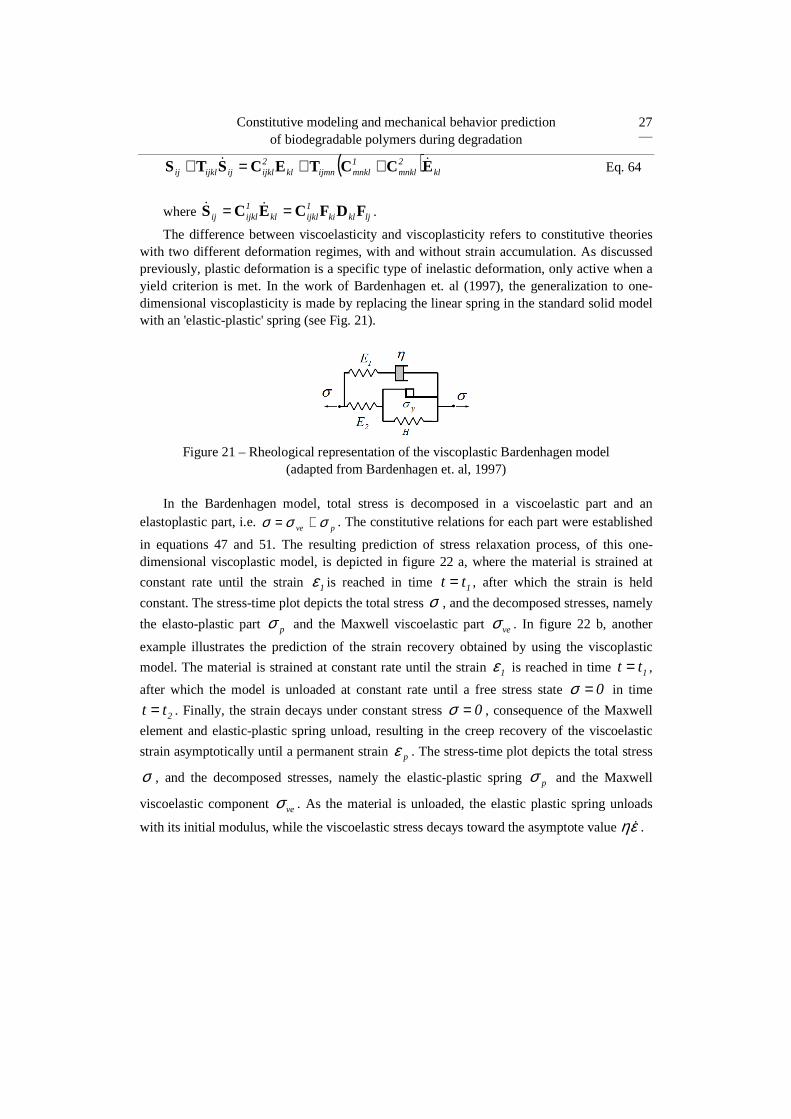
The difference between viscoelasticity and viscoplasticity refers to constitutive theories with two different deformation regimes, with and without strain accumulation. As discussed previously, plastic deformation is a specific type of inelastic deformation, only active when a yield criterion is met. In the work of Bardenhagen et. al (1997), the generalization to one-dimensional viscoplasticity is made by replacing the linear spring in the standard solid model with an 'elastic-plastic' spring (see Fig. 21).

Figure 21 – Rheological representation of the viscoplastic Bardenhagen model

(adapted from Bardenhagen et. al, 1997) In the Bardenhagen model, total stress is decomposed in a viscoelastic part and an

elastoplastic part, i.e. pve σσσ += . The constitutive relations for each part were established

in equations 47 and 51. The resulting prediction of stress relaxation process, of this one-dimensional viscoplastic model, is depicted in figure 22 a, where the material is strained at

constant rate until the strain 1ε is reached in time 1tt = , after which the strain is held

constant. The stress-time plot depicts the total stress σ , and the decomposed stresses, namely

the elasto-plastic part pσ and the Maxwell viscoelastic part veσ . In figure 22 b, another

example illustrates the prediction of the strain recovery obtained by using the viscoplastic

model. The material is strained at constant rate until the strain 1ε is reached in time 1tt = ,

after which the model is unloaded at constant rate until a free stress state 0=σ in time

2tt = . Finally, the strain decays under constant stress 0=σ , consequence of the Maxwell

element and elastic-plastic spring unload, resulting in the creep recovery of the viscoelastic

strain asymptotically until a permanent strain pε . The stress-time plot depicts the total stress

σ , and the decomposed stresses, namely the elastic-plastic spring pσ and the Maxwell

viscoelastic component veσ . As the material is unloaded, the elastic plastic spring unloads

with its initial modulus, while the viscoelastic stress decays toward the asymptote value εη ɺ .


Figure 22 – Example of strain histories and corresponding stress-strain response of the viscoplastic model (adapted from Bardenhagen et al., 1997)

Another common approach to model the viscoelastic-plastic behavior is to consider, as

Perzyna (1966), the total strain or the strain rate to be sum of several components. Instead of the stress decomposition here shown for the standard solid model, these other approaches consider the strain (or strain-rate) decomposition into elastic and inelastic (or viscoplastic) components acting in series (see the rheological representation in figure 23):

vpe εεε += Eq. 65

The constitutive relation for the elastic part eε is the Hooke’s law, which establishes a

linear relation between stress and strain, εe=σ/E. For the viscoplastic component, the viscous and the plastic strain is the same, i.e. εvp= εv= εp. Furthermore, total viscoplastic stress can be decomposed into viscous σv and plastic σp stresses:

yvp

pvvp dt

dσ

εησσσ +=+= Eq. 66

Then:

pvpyvp

vpyvp 0

εεσσεσσ

=⇒>

=⇒< Eq. 67

However, this simple model is unable to simulate the viscoelastic behavior below

yielding.

a)

b)


29

Figure 23 – Rheological representation of the viscoplastic Perzyna model.

More complex variants of these simple models can be found at the literature (Arruda and

Boyce, 1993b; Bardenhagen et al., 1997; Bergström et al., 2002; Boyce et al., 1988; Dafalias, 1991; Drozdov and Gupta, 2003; Fancello et al., 2006; Harren, 1995; Hasan and Boyce, 1995; Hausler and Sayir, 1995; Holzapfel, 1996; Johnson et al., 1995; Lubarda et al., 2003; O'Dowd and Knauss, 1995; Reese and Govindjee, 1998; Rubin, 1987; Zdunek, 1993). Those models can simulate the non linear viscoelastic, viscoplastic and hysteretic response of polymers. In fact, they are based on the same concept of networks, combining elastic, sliding and dissipative elements, in order to simulate the time-dependent response of the material, based on the Boltzmann superposition principle. Generally, a more complex model is more precise to simulate the mechanical behavior. On the other hand, also the inverse parameterization is more complex, since additional mechanical test are needed to identify all the material parameters (monotonic tests at different rates; cyclic, creep and relaxation tests, etc). The selection of an adequate model depends on the simulation needs. If the aim is to simulate the mechanical behavior of biodegradable polymers at low deformations and a specific deformation rate, the linear elastic or the Neo-Hooke model is accurate enough. However, if the aim is to study the mechanical behavior at moderate deformation in a small range of deformation rates, the best choice is a linear viscoelastic model, considering hyperelastic constitutive relations for the spring elements. Thus, if the aim is to simulate the mechanical behavior of the biodegradable polymer submitted to a generic load spectrum, considering a large range of deformation rates and large deformations, a more complex viscoelastic or viscoplastic model is needed.

The Bergström-Boyce model (Bergström and Boyce, 1998) is a viscoelastic model, which simulates the performance of polymers undergoing large deformations. It can be calibrated through a relative small set of simple mechanical tests, such as uniaxial loading, to provide accurate predictions for different loading cases (Bergström et al., 2002). These comprise monotonic loading under different strain rates, including hysteresis effect, and unloading-reloading cycles at different strain levels (Bergström et al., 2002). In this constitutive model, the mechanical behavior is decomposed into two parts: a time-independent response, modeled by a hyperelastic constitutive model (defined as Network A), and a time-dependent deviation from equilibrium relaxed configuration, defined by an inelastic constitutive model (defined as Network B) as shown by figure 24. In fact, the Network B is composed of an elastic element (also modeled by a hyperelastic constitutive model) in series with a time-dependent element, which acts to relieve the strain of the Network A in function of the time. According to the rheological representation of the constitutive model, shown in figure 24, the material behavior is modeled as two polymer networks acting in parallel (Bergström and Boyce, 1998).


Figure 24 – Rheological representation adapted from Bergström and Boyce (1998).

Since deformation in Network A is the same of Network B, then F=FA=FB. The

deformation gradient in Network B can be further decomposed into an inelastic deformation followed by an elastic deformation (FB=Fe

BFiB), where the inelastic deformation represents

the configuration obtained by a complete virtual elastic unloading of Network B until a stress free state. The stress response of Network A is given by the Arruda-Boyce model (Arruda and Boyce, 1993b). A different form of equation 35 is:

( ) ij*ij

L1

L*1

*

Aij 1J'

)/1(

)/(

Jδκ

λλλ

λµ −+= −

−

BTL

L Eq. 68

where µ is the shear modulus, κ is the bulk modulus, and λL is the limiting chain stretch.

ℒ−1(x) is the inverse Langevin function, where ℒ(x)=[coth(x) − 1/x]. *λ is the applied chain

stretch, which can be calculated from:

( )3

*ij* Btr

=λ Eq. 69

where B*=J-2/3B= J-2/3FFT. The stress on Network B is also given by the eight-chain

model:

( ) ij*ij

L1

L

*eB

1

*eB

eB

Bij 1J'

)/1(

)/(

J

s δκλλλ

λ

µ −+= −

−

BTL

L Eq. 70

where s is a dimensionless material parameter, which specifies the shear modulus of

Network B relative to Network A, and *e

Bλ is the chain stretch in the elastic part of Network

B. Using this representation, the total Cauchy stress tensor is given by T=TA+TB.

The velocity gradient in Network B, 1

BBB−= FFL ɺ (see definition in Appendix), and the

deformation gradient in Network B can be decomposed into elastic and inelastic components

( iB

eBB FFF = ). Hence:


31

( ) ( ) [ ]( ) ( )( ) ( ) ( ) ( ) i

BeB

1eB

iB

eB

eB

1eB

1iB

iB

eB

1eB

eB

1eB

1iB

iB

eB

iB

eB

1iB

eB

iB

eBB

~dt

d

LLFLFLFFFFFF

FFFFFFFFFFL

+=+=+=

=+=

=

−−−−

−−−

ɺɺ

ɺɺ

Eq. 71

where the velocity gradient L can be decomposed into the sum of stretch rate and spin

tensors, D and W, respectively:

( ) iB

iB

1iB

iB

iB WDFFL +== −ɺ Eq. 72

iB

iB

iB

~~~WDL += Eq. 73

The unloading process, which relates the deformed state with the intermediate relaxed

state, is not uniquely defined; since an arbitrary rigid body rotation of the intermediate state still leaves the state stress free (Bergström et al., 2002). To ensure the unloading unique, the

viscous spin tensor is prescribed zero, i.e. ≡iB

~W 0, according to the researchers (Bergström

and Boyce, 1998; Bergström et al., 2002). The rate of viscoplastic deformation of Network B is constitutively prescribed by:

( ) ( ) 1eB

1iB

iB

eB

BB

iB

iB

'~~ −−=== FFFFT

DL ɺɺ

τγ Eq. 74

where [ ]BB '' TTtr=τ is the effective stress, which drives the viscous flow. The time

derivative of iBF can be derived as follows:

( ) iB

eB

B1eBB

iB

'FF

TFF

τγ −= ɺɺ Eq. 75

The effective creep rate-equation for viscous flow is given by the literature (Bergström

and Boyce, 1998; Bergström et al., 2002):

( )m

cutbase

CiB0B ˆ1

−+−= τ

ττξλγγ ɺɺ Eq. 76

where 0γɺ =1(s-1) is a constant introduced to ensure dimensional consistency. cutτ̂ is a cut-

off stress such that no flow will occur for values lower than the cut-off stress. baseτ represents

the flow resistance. m is a positive stress exponential. ξ is a strain adjustment factor, and C is

a strain exponential constant, which is restricted at the interval [-1, 0]. The chain stretch in the inelastic part of Network B is given by Bergström and Boyce (1998):


[ ]3

TiB

iBi

B

FFtr=λ Eq. 77

In the figure 25, it is possible to observe that the evaluated viscoplastic model was able to

simulate the time-dependent response of the polymer in this range of strain rates (500 mm/min and 15 mm/min). By using these two loading cases in the inverse analyses, the coefficient of determination R2 was very close to 1(one), meaning that the model was able to predict very accurately the mechanical behavior of the polymer at different strain rates. In the figure 25, it is verified that the evaluated viscoplastic model was also able to simulate the hysteric effect, commonly observed in polymers. By using cyclic unloading-reloading and monotonic loading cases in the inverse analyses, the coefficient of determination R2 was still very close to 1(one).

Figure 25 – Experimental results of a) monotonic tensile test at two strain rates (500 and 15

mm/min) and b) cyclic tensile test of a biodegradable polymer (PLA-PCL), and prediction via Bergström-Boyce model (adapted from Vieira et. al, 2014).

In a recent study (Muliana and Rajagopal, 2012), a non linear viscoelastic model was

used to model the time-dependent performance of biodegradable structures. In that work, the authors considered that hydrolytic damage depends both on the deviatoric strain tensor and on the concentration of water. Hence, at each time increment step, damage must be calculated in the material point. First water concentration at each material point is updated based on Fick’s law. Then the hydrolytic damage is updated as function of the deviatoric strain tensor. Finally, the constitutive relation is updated at each time increment step. This method enables to model the relaxation behavior (or creep) during degradation, and it is reasonably good to model moderate deformations. Later, Khan and El-Sayed (2013) developed a phenomenological constitutive viscoelastic-plastic model able to predict the response of biodegradable polymers under large deformations. The model consists of nonlinear elastic spring acting in parallel with a variable number of Maxwell elements. The hyperelastic response of the springs both in the elastic branch and in the Maxwell branch is governed by the Ogden-type free energy function. More recently, Vieira et al. (2014) used the Bergstrom-Boyce model in a similar approach, where some of the material parameter depends on the degradation damage. Since this constitutive model has 9 material parameters, a parametric study was preformed to evaluate the most sensitive parameters. The shear modulus µ and the

a) b)


33

flow resistance τbase are the most sensitive parameters, while the predicted results are almost insensible to deviations of 10% of the other parameters. After determining the two most sensitive parameters at each degradation step, they were fitted by linear regression as function of the degradation damage d(t,u), while the other parameters were set constant during the hydrolytic degradation process, assuming averaged values identified from the different hydrolytic degradation steps. It was observed that the shear modulus decreases nearly linear as function of the hydrolytic damage. This same trend was also shown in this chapter and was also reported in a previous work (Vieira et al., 2011a), where the neo-Hookean, Mooney-Rivlin and second reduced hyperelastic models were used to predict the mechanical behavior of the same biodegradable polymer. Muliana and Rajagopal (2012) also assumed in their own viscoelastic model that shear modulus decreases with hydrolytic degradation, i.e. hydrolytic degradation process softens the polymers. On the order hand, Soares (2008) reported that the material becomes less viscous during hydrolytic degradation, and returns faster to a relaxed state. This assumption is also consistent to the results found in the work of Vieira et al. (2014), where the flow resistance τbase increases nearly linearly with the hydrolytic damage. Based on these linear equations (see figure 26), the shear modulus µ(d) and the flow resistance τbase(d), with other material model parameters values previously set constant during hydrolytic degradation, the mechanical behavior of the polymer was predicted at different degradation steps. In the figure 27, the experimental results are compared against predictions using this method.

Figure 26 – Evolution of the material parameters of the Bergtröm-Boyce model, shear

modulus µ and flow resistance τbase, during hydrolytic degradation.

This type of approach allows the four-dimensional modeling, where the fourth dimension is the time. However, the characteristic time of degradation is different from the characteristic viscoelastic time for stress relaxation or creep. If the material has viscoelastic attributes, then the degradation time-dependent phenomenon couples with the time-dependent mechanical behavior of the material. Stretching induces stress relaxation with time by means of viscous flow of the material, and in parallel, it induces chemical scissions of the molecules that provide an additive pathway for relaxation. Hence, if a stress field is applied during degradation, a five-dimensional modeling should be considered.



and model results via viscoplastic Bergström-Boyce model, after 0, 2, 4 and 8 weeks of hydrolytic degradation.

CONCLUSIONS Biodegradable polymers, as conventional polymers are known by their non-linear and

time-dependent mechanical behavior, as shown by the experimental results. The presented methods, for which some material parameters (the most sensitive) depend on the degradation damage, enable the simulation of the mechanical behavior during hydrolytic degradation. Depending on the simulation needs, different models (such as linear elastic, hyperelastic, elastoplastic, viscoelastic and viscoplastic) with different degrees of complexity may be used to predict the three-dimensional mechanical behavior of biodegradable polymers at each degradation step. These constitutive models can be implemented in commercial finite element software applied to complicated numerical models in 3D applications. Hence, this type of approach can provide new insights to the design and dimensioning of biodegradable devices, such as scaffolds, according to mechanical and durability requirements. Furthermore, it enables the pre-validation of functional compatibility of biodegradable implantable medical devices.

ACKNOWLEDGMENTS André C. Vieira wishes to thank CAPES/CNPq (Young Talents Program – grant number:

022/2012). The authors would like to highlight that this work was also partially supported by the Program USP/UP, which is a scientific cooperation agreement established between the University of Porto (Portugal) and the University of São Paulo (Brazil). The author Rui M.


35

Guedes also acknowledge the support under the grant PTDC/EME-PME/114808/2009 provided FCT (Portuguese Science and Technology Foundation).

REFERENCES Arruda, E.M., Boyce, M.C., 1993a. Evolution of plastic anisotropy in amorphous polymers

during finite straining. Int. J. Plast. 9, 697-720. Arruda, E.M., Boyce, M.C., 1993b. A three-dimensional constitutive model for the large

stretch behavior of rubber elastic materials. J. Mech. Phys. Solids 41(2), 389-412. Bardenhagen, S.G., Stout, M.G., Gray, G.T., 1997. Three-dimensional, finite deformation,

viscoplastic constitutive models for polymeric materials. Mech. Mater. 25, 235-253. Bergström, J., Boyce, M.J., 1998. Constitutive modeling of the large strain time-dependent

behavior of elastomers. Mech. Phys. Solids. 46, 931-954. Bergström, J.S., Kurtz, S.M., Rimnac, C.M., Edidin, A.A., 2002. Constitutive modeling of

ultra-high molecular weight polyethylene under large-deformation and cyclic conditions. Biomaterials 23, 2329–2343.

Bellenger, V., Ganem, M., Mortaigne, B., Verdu, J., 1995. Lifetime prediction in the hydrolytic ageing of polyesters. Polym. Degrad. Stab. 49, 91–97.

Bird, R.B., Armstrong R.C., Hassager,O., 1977. Dynamics of polymeric liquids: Vol. I. John Wiley and Sons, New York.

Boyce, M.C., Parks D.M., Argon A.S., 1988. Large inelastic deformation of glassy polymers. I. Rate dependent constitutive model. Mech. Mater. 7, 15-33.

Chagnon, G., Marckmann, G., Verron, E., 2004. A comparison of the Hart-Smith model with Arruda- Boyce and Gent formulations for rubber elasticity. Rubber Chem. Technol. 77(4), 724-735.

Chu, C.C., 1985. Strain-accelerated hydrolytic degradation of synthetic absorbable sutures. In: Hall, C.W. (Eds.). Surgical Research, Recent Developments: Proceedings of the First Annual Scientific Session of the Academy of Surgical Research, Pergamon Press, San Antonio, pp. 111–115.

Dafalias, Y.F., 1991. Constitutive model for large viscoelastic deformations of elastomeric materials. Mech. Res. Commun. 18, 61–66.

Drozdov, A.D., Gupta, R.K., 2003. Constitutive equations in finite viscoplasticity of semicrystalline polymers. Int. J. Solids Struct. 40, 6217–6243.

Fancello, E., Ponthot, J.P., Stainier, L., 2006. A variational formulation of constitutive models and updates in non-linear finite viscoelasticity. Int. J. Numer. Meth. Eng. 65, 1831–1864.

Farrar, D.F., Gilson, R.K., 2002. Hydrolytic degradation of polyglyconate B: the relationship between degradation time, strength and molecular weight. Biomaterials 23, 3905–3912.

Ferry, J.D., 1980. Viscoelastic Properties of Polymers, John Wiley and Sons, New York. Flory, P.J., Rehner, J., 1943. Statistical Mechanics of Cross‐Linked Polymer Networks I.

Rubberlike Elasticity. J. Chem. Phys. 11(11), 512-520. Forni, M., Martelli, A., Dusi, A., 1999. Implementation and Validation of Hyperelastic Finite

Element Models of High Damping Rubber Bearings. In: Dorfmann, A., Muhr, A., (Eds.). Constitutive Models for Rubber, AA Balkema Publishers, Rotterdam, pp.237-247.

Garlotta, D.A., 2001. Literature Review of Poly(Latic Acid). J Polym. Environ. 9, 63-84.


Gan, Z., Yu, D., Zhong, Z., Liang, Q., Jing, X., 1999. Enzymatic degradation of poly(ε-caprolactone)/poly(DL-lactide) blends in phosphate buffer solution. Polymer. 40, 2859–2862.

Ghosh, P., Saha, A., Mukhopadhyay, R., 2003. Prediction of tyre Rolling Resistance Using FEA. In: Busfield, J., Muhr, A.H., (Eds.). Constitutive Models for Rubber III, Swets &Zeitlinger, Lisse, pp. 141-145.

Göpferich, A., 1996. Mechanisms of polymer degradation and erosion. Biomaterials 17, 103–114.

Göpferich, A., Langer, R., 1993. Modeling of polymer erosion. Macromolecules 26, 4105–4112.

Grabow, N., Bunger, C.M., Sternberg, K., 2007. Mechanical properties of a biodegradable balloon-expandable stent from poly (L-lactide) for peripheral vascular application. ASME J. Med. Devices. 1, 84–88.

Harren, S.V., 1995. Toward a new phenomenological flow rule for orientationally hardening glassy polymers, J. Mech. Phys. Solids. 43, 1151-1173.

Hasan, O.A., Boyce, M.C., 1995. A Constitutive Model for the Nonlinear Viscoplastic Behavior of Glassy Polymers. Polym. Eng. Sci. 35, 331-344.

Hausler, K., Sayir, M.B., 1995. Nonlinear viscoelastic response of carbon black reinforced rubber derived from moderately large deformations in torsion. J. Mech. Phys. Solids. 43, 295–318.

Herzog, K., Muller, R.-J., Deckwer, W.-D., 2006. Mechanism and kinetics of the enzymatic hydrolysis of polyester nanoparticles by lipases. Polym. Degrad. Stab., 91, 2486–2498.

Holzapfel, G., 1996. A new viscoelastic constitutive model for continuous media at finite thermomechanical changes. Int. J. Solids Struct. 33, 3019–3034.

Huntley, H.E., Wineman, A.S., Rajagopal, K.R., 1996. Chemorheological relaxation, residual stress and permanent set arising in radial deformation of an elastomeric hollow sphere. Math. Mech. Solids, 1, 267–299.

Johnson, A.R., Quigley, C.J., Freese, C.E., 1995. A viscohyperelastic finite element model for rubber. Comput. Methods. Appl. Mech. Eng. 127, 163–180.

Khan, K.A., El-Sayed, T., 2013. A phenomenological constitutive model for the nonlinear viscoelastic responses of biodegradable polymers. Acta Mech. 224(2):287-305.

Krynauw, H., Bruchmüller, L., Bezuidenhout, D., Zilla, P., Franz, T., 2011. Constitutive modelling of degradation induced mechanical changes in a polyester-urethane scaffold for soft tissue regeneration. In: Fernandes P.R. et al. (Eds).. Proceedings of II International Conference on Tissue Engineering, June 2-4, Lisbon.

Li, S., Garreau, H., Vert, M., 1990. Structure-property relationships in the case of the degradation of massive aliphatic poly (α-hydroxyacids) in aqueous media. Part 2: degradation of lactide/glycolide copolymers: PLA37.5GA25 and PLA75GA25. J. Mater. Sci.-Mater. M. 1, 131–139.

Lubarda, V.A., Benson, D.J., Meyers, M.A., 2003. Strain-rate effects in rheological models of inelastic response. Int. J. Plast. 19, 1097–1118.

Lunt, J., 1998. Large-scale Production, Properties and applications of Polylatic Acid Polymers. Polym. Degrad. Stab. 59, 145-152.

Malvern, L.E., 1969. Introduction to the Mechanics of a Continuous Medium. Prentice-Hall, Englewood Cliffs.


37

Miller, N.D., William, D.F., 1984. The in vivo and in vitro degradation of poly(glycolic acid) suture material as a function of applied strain. Biomaterials. 5, 365-368.

Moore, J.E., Soares, J.S., Rajagopal, K.R., 2010. Biodegradable stents: biomechanical modeling challenges and opportunities. Cardiovascul. Eng. Technol. 1, 52-65.

Muliana, A., Rajagopal, K., 2012. Modeling the response of nonlinear viscoelastic biodegradable polymeric stents. Int. J. Solids. Struct., 49(7-8), 989-1000.

Nikolic, M.S., Poleti, D., Djonlagic, J., 2003. Synthesis and characterization of biodegradable poly(butylenes succinate-co-butylene fumarate)s. Eur. Polym. J., 39, 2183-2192.

O'Dowd, N.P., Knauss, W.G., 1995. Time dependent large deformation of polymers, J. Mech. Phys. Solids. 43, 771-792.

Perzyna, P., 1966. Fundamnental problems in viscoplasticity, Adv. Appl. Mech. 9, 243-377. Rajagopal, K.R., Srinivasa, A.R., Wineman, A.S., 2007. On the shear and bending of a

degrading polymer beam. Int. J. Plast. 23, 1618–1636. Rajagopal, K.R., Wineman, A.S., 1992. A constitutive equation for nonlinear solids which

undergo deformation induced microstructural changes. Int. J. Plast. 8, 385–395. Raoult, I., Stolz, C., Bourgeois, M., 2005. A Constitutive Model for the Fatigue Life

Prediction of Rubber. In: Austrell, P.E., Kari, L., (Eds.) Constitutive Models for Rubber IV, Taylor & Francis Group, London, pp. 129-134.

Reese, S., Govindjee, S., 1998. A theory of finite viscoelasticity and numerical aspects. Int. J. Solids Struct. 35, 3455–3482.

Rubin, M.B., 1987. An elastic-viscoplastic model exhibiting continuity of solid and fluid states. Int. J. Eng. Sci. 9, 1175-1191.

Shaw, J.A., Jones, A.S., Wineman, A.S., 2005. Chermorheological response of elastomers at elevated temperatures: experiments and simulations. J. Mech. Phys. Solids 53, 2758–2793.

Smeulders, S.B., Govindjee, S., 1999. A phenomenological model of an elastomer with an evolving molecular weight distribution. J. Rheol. 43, 393-414.

Soares, J.S., 2008. Constitutive Modeling for Biodegradable Polymers for Applications in Endovascular Stents. PhD Dissertation. Mechanical Engineering Texas A&M University.

Soares, J., Rajagopal, K.R., Moore J.E., 2010. Deformation induced hydrolysis of a degradable polymeric cylindrical annulus. Biomech. Model Mechan. 9(2), 177-186.

Treloar, L.R.G.. 1975. The Physics of Rubber Elasticity. Oxford University Press, Oxford. Treloar, L.R. G.. 1946. The elasticity of a network of long-chain molecules-III. Trans.

Faraday Soc. 42, 83-94. Tsuji, H., Ikada, Y., 1998. Properties and morphology of poly(Llactide)—II hydrolysis in

alkaline solution. J. Polym. Sci. A Polym. Chem. 36, 59–66. Tsuji, H., Ikada, Y., 2000. Properties and morphology of poly(Llactide) 4. Effects of

structural parameters on long-term hydrolysis of poly(L-lactide) in phosphate-buffered solution. Polym. Degrad. Stab. 67, 179–189.

Tsuji, H., Nakahara, K., 2001. Poly(L-lactide)—IX hydrolysis in acid media. J. Appl. Polym. Sci. 86, 186–194.

Vieira, A.C, Vieira J.C., Ferra J., Magalhães F.D., Guedes R.M., Marques A.T., 2011a). Mechanical study of PLA–PCL fibres during in vitro degradation. J. Mech. Behav. Biomed. 4(3), 451-60.


Vieira, A.C., Marques, A.T., Guedes, R.M., Tita, V., 2011b). Material model proposal for biodegradable materials. Procedia Engineering 10, 1597–1602.

Vieira, A.C., Medeiros, R., Guedes, R.M., Marques, A.T., Tita, V., 2013. Visco-Elastic-Plastic Properties of Suture Fibers Made of PLA-PCL. Materials Science Forum. 730-732, 56-61.

Vieira, A.C., Guedes, R.M., Tita, V., 2014. Constitutive modeling of biodegradable polymers: Hydrolytic degradation and time-dependent behavior. Int. J. Solids Struct. 51, 1164–1174.

Wang M.C., Guth E., 1952. Statistical Theory of Networks of Non‐Gaussian Flexible Chains. J. Chem. Phys. 20(7), 1144-1157.

Ward, I.M., 1979. Mechanical Properties of Solid Polymers. John Wiley and Sons, New York.

Williams, D.F., 1981. Enzymatic hydrolysis of polylactic acid. Proc Inst Mech Eng H 10, 5–7.

Wineman, A., Min, J.H., 2002. Time-dependent scission and cross-linking in an elastomeric cylinder undergoing circular shear and heat conduction. Int. J. Nonlinear Mech. 38, 969–983.

Zdunek, A.B., 1993. Theory and computation of the steady state harmonic response of viscoelastic rubber parts. Comput. Methods Appl. Mech. Eng. 105, 63–92.


39

APPENDIX

Description of shape changes in solids An external force applied to solid results in a displacement, which can be divided into

two components: • A rigid-body displacement: in this case, the relative displacement between particles

is zero, i.e. the shape and size of the body does not change. • A deformation: in this case, there is a relative displacement between particles, i.e. the

shape is changed. For materials undergoing large deformations, such as polymers, finite strain theory must

be applied. In this section of the Appendix, the various mathematical formulas, which are used to characterize shape changes in solids, are shown.

Let Xi denotes the components of a Cartesian vector, specifying a material point in the reference configuration. Then xi(Xi,t) denotes the same material point in the deformed configuration, and represents the position of this material point at time t.

Hence, the displacement vector, ui, is defined as:

( )t,iiii XuXx += Eq. A1

and the displacement gradient (in the Lagrangean description) is a second order tensor

defined as:

j

iij X

uU

∂∂= Eq. A2

Then the deformation gradient F, in the so-called Lagragian description (i.e. position in

the deformed configuration depends on the position of the same material point in a fixed referential coordinates), is a second order tensor defined by:

j

iij X

xF

∂∂= Eq. A3

and the deformation gradient can also be expressed as:

j

iijij X

uUIF

∂∂+=+= δ Eq. A4

where I is the identity tensor, with components described by the Kronecker delta symbol:

=≠

=ji,1

ji,0ijδ Eq. A5


The other description for motion is made in terms of the current coordinates, called the Eulerian description. The difference between these two descriptions is that, in the Eulerian description, one places the coordinate system on the solid as it moves, while in the Lagrangian description, the motion of the solid is described from a fixed coordinate system. The inverse of the deformation gradient, or the deformation gradient, in the Eulerian description, arises in many calculations.

j

i1ij x

XF

∂∂=−

Eq. A6

The Jacobian is defined as the determinant of the deformation gradient:

0ij dV

dVJ == F Eq. A7

and it is a measure of the volume change produced by a deformation, where V is the

current volume and V0 is the initial volume. Hence, for any physically admissible deformation, the volume of the deformed element must be positive (i.e. J > 0). If a material is incompressible, its volume remains constant (i.e. J=1).

The Lagrangian strain tensor is measured with respect to the initial configuration (i.e., Lagrangian description) and it is another way to describe the shape change of a solid. It is defined as:

( ) ( )IFFFFE −=−= .2

1

2

1 Tijkjkiij δ Eq. A8

Thus, because j

iijij X

uF

∂∂

+= δ the relationship between Lagrangian strain and

displacement is given by:

∂∂

∂∂+

∂∂

+∂∂=

j

k

i

k

i

j

j

iij 2

1

Xu

Xu

X

u

Xu

E Eq. A9

The Eulerian strain tensor is measured with respect to the deformed or current

configuration (i.e. Eulerian description). It is defined as:

( ) ( )

∂∂

∂∂+

∂∂

+∂∂=−=−= −−−−

j

k

i

k

i

j

j

i1T1kj

1kiij

*ij 2

1.

2

1

2

1

xu

xu

x

u

xu

FFIFFE δ Eq. A10

There are two other deformation tensors, which are often encountered in the finite strain

theory. The right and left Cauchy-Green deformation tensors, which are respectively defined by:


41

FFFFC .Tkjkiij == Eq. A11

Tjkikij .FFFFB == Eq. A12

Other important second order tensors, which are used to describe the shape change in

solids, the right stretch tensor, the left stretch tensor and the rotation tensor are respectively defined by:

( )21

21

kjkiijij FFCU == Eq. A13

( )21

21

jkikijij FFBV == Eq. A14

kj1

ik1

kjikij FVUFR −− == Eq. A15

Hence, the multiplicative decomposition of the deformation gradient can be regarded as a

sequence of two homogeneous deformations, stretch U followed by a rigid rotation R:

kjikij URF = Eq. A16

Similarly, the deformation gradient can be regarded as a sequence a rotation R followed

by of stretch V:

kjikij RVF = Eq. A17

It important to retain that R orthogonal ( IRRRR == TT .. ), therefore, represents a

rotation ( =R 1).

The principal stretches λ1, λ2 and λ3 are the eigenvalues of F, U or V, or they are the square root of the eigenvalues of C and B. Hence, there are two sets of principal stretch directions. The principal stretch directions associated to the reference configuration are the eigenvectors of U and C. On the other hand, the principal stretch directions associated to the current configuration are the eigenvectors of V and B. The relation between these two sets of principal directions is the rotation tensor R.

The velocity is a vector that describes the rate of position changes of the material points:

( ) ( )t

t,

t

t, iii ∂

∂=∂

∂= XxXuv Eq. A18

And the velocity gradient (in the Lagrangean description) is a second order tensor defined

as:

j

iij X

vL

∂∂= Eq. A19

The velocity gradient can be expressed in terms of the deformation gradient and its time

derivative as:


11

kjikij . −− == FFFFL ɺɺ Eq. A20

The stretch rate and the spin second order tensors are defined, respectively, as:

( ) ( ) 2/2/ Tjiijij LLLLD +=+= Eq. A21

( ) ( ) 2/2/ Tjiijij LLLLW −=−= Eq. A22

Hence, velocity gradient can be decomposed into the sum of stretch rate and spin, as:

ijijij WDL += Eq. A23

The rate of deformation tensor can be related to time derivatives of other strain measures.

For example, the time derivative of the Lagrange strain tensor can be shown to be:

FDFFDFE ..Tljklkiij ==ɺ Eq. A24

Description of internal forces in a solid Stress is a measure of the average amount of force exerted per unit area and it is a

reaction to external forces on a surface of a body. The stress vector ti at a material point represents the force Fi acting on the surface per unit area A:

i

ii dA

dFt = Eq. A25

The resultant force acting on any portion S of the surface of the deformed solid is:

∫=S

iii dAtF Eq. A26

To elaborate further on this concept, consider a small cube in the body as depicted in

figure A1.


43

Figure A1 – Elementary cube representing the stress tensor

Let the stress vector that acts on the surface dA3 be t3, where n3 = (0, 0, 1) is the normal unit vector. t3 may be decomposed into three components in the direction of the coordinate axes and denote them by T31, T32 and T33. Similarly, it is possible to consider surface dA1 and dA2 perpendicular to 1 and 2, the stress vectors acting on them t1, t2, and their components in the 1, 2 and 3 directions. The components T11, T22 and T33 are called normal stresses, and T12, T13, T21, T23, T31 and T32 are called shear stresses. Then, the Cauchy stress tensor is defined by:

=

=

333231

232221

131211

3

2

1

ij

TTT

TTT

TTT

t

t

t

T Eq. A27

Cauchy stress tensor relates forces in the current (i.e. deformed) configuration to areas in

the current configuration. Hence, sometimes the Cauchy stress tensor is also called the true stress tensor. It completely characterizes the internal forces acting in a deformed solid. In addition, the Cauchy stress tensor is symmetric, which is implied from the fact that the equilibrium of an element requires that the resultant moment vanish.

Other definitions of stress often appear in constitutive equations. The first Piola-Kirchhoff stress tensor relates forces in the current configuration with areas in the initial configuration. In general, the first Piola-Kirchhoff stress tensor is not symmetric. The transpose of the first Piola-Kirchhoff stress tensor is also called the nominal stress tensor. The relationship between the first Piola-Kirchhoff stress tensor Pij and the Cauchy stress tensor Tij

is given by:

T1jiijij ..J −− == FTFFTP Eq. A28

The Kirchhoff stress refers to a weighted Cauchy stress tensor and it is defined by:

TFTK .J ijij == Eq. A29


Finally, the second Piola-Kirchhoff stress tensor relates forces in the initial configuration to areas in the initial configuration. The relationship between the second Piola-Kirchhoff stress tensor S and the Cauchy stress tensor �ij is given by:

TT1

jlkl1

ikij ...J −−−− == FTFFFTFS Eq. A30

The stress measures are work-conjugate to particular strain measures. This means that the

rate of work done by the forces can be calculated by a stress measure multiplied by the time derivative of the conjugated strain measure. The rate of work done by stresses acting on a small material element with volume dV0 in the undeformed solid (and volume dV in the deformed solid) can be computed as:

0ijij0ijij0ijijijij dVdVdVdVW SEPFKDTD ɺɺɺ ==== Eq. A31

onstitutive modeling and mechanical behavior … · 2019-07-14 · constitutive modeling and...

Documents