online temporal signal comparison

Online Temporal Signal Comparison Using Singular Points Augmented TimeWarping

Rajagopalan Srinivasan*,†,‡ and Mingsheng Qian†

Laboratory for Intelligent Applications in Chemical Engineering, Department of Chemical andBiomolecular Engineering, National UniVersity of Singapore, 10 Kent Ridge Crescent, Singapore 119260,and Process Sciences and Modeling, Institute of Chemical and Engineering Sciences, 1 Pesek Road,Jurong Island, Singapore 627833

Advances in instrumentation and data storage technologies have allowed the process industries to collectextensive operating data which can be used to extract information about the underlying process and provideonline decision support. One of the fundamental problems in data-based decision support is comparison oftime-series data. Many signal comparison methods require signals that are of the same length and synchronized.Synchronization of varying length signals is usually achieved using dynamic time warping (DTW). Majorlimitations of DTW include computational cost and the tendency to link operationally different points.Previously, we proposed singular points augmented time warping to overcome these shortcomings duringoffline signal comparison (Srinivasan and QianInd. Eng. Chem. Res.2005, 44, 4697). Landmarks in processdata such as extreme values and sharp changes, called singular points, are used to segment a signal intoregions with homogeneous properties, called episodes. Singular points of two signals are linked by dynamicprogramming; time warping is used to synchronize the episodes. A locally optimal equivalent of DTW calledextrapolative time warping (XTW) with better computational performance was also proposed. In this paper,we present the extension of this approach to online signal comparison. The online signal comparison problemis a generalization of the offline problem and has two additional challenges: (1) the reference signal forcomparison is not known a priori and has to be selected from a library, and (2) the starting point of thereference and real-time signal would not coincide in general, and the corresponding points have to be identified.The approach proposed here addresses these by extending dynamic locus analysis (Srinivasan and QianChem.Eng. Sci.2006, 61, 6109) and singular point augmented XTW using anchoring and flanking strategies. Theapplication of the proposed approach is illustrated using two different case studies: online operating modeidentification in the Tennessee Eastman process and online fault identification in a lab-scale distillation column.The results show that the proposed approach is robust, efficient, and suitable for online signal comparison.

1. Introduction

As a result of significant advances in data collection andstorage, vast amounts of historical operating data are becomingcommonly available in the chemical process industry. Thisdata is a rich source of information about the process that canbe used to improve the plant operation. Given the paralleldevelopments in pattern classification3 and statistical, informa-tion, and systems theories,4 data-based approaches have beengaining in popularity. Potential areas of application of data-driven methods include regulatory and sequence control,visualization, operation improvement, state identification, andfault diagnosis. Despite these developments in extractinginformation and knowledge from data, many important andchallenging problems persist in data analysis and knowledgeextraction. In this paper, we address one such problem: onlinetemporal signal comparison.

Temporal signals with time-varying properties commonlyarise in chemical plants during transition states such as startup,grade change, shutdown, maintenance, and other abnormaloperations. The precept of signal comparison-based approachesis that similar states result in similar temporal signals. So, if ahistorical database of representative signals is available, the rootcause of a process change occurring in real-time can be

determined. The challenge, however, is that, as a result of thenature of industrial operations, signals from different instancesof the same state are not exact replicates; there would besignificant differences in magnitude and duration of the variableprofiles as a result of run-to-run variations arising from differinginitial conditions, impurities, seasonal affects, and operatoractions. A direct comparison of a real-time signal with areference signal in the historical database would therefore beincorrect, and signal comparison methods try to account for thesenormal operational variations.

1.1. Previous Work in Online Signal Comparison.Threeclasses of signal comparison methods can be differentiated. Thefirst class of methods is based on multivariate statisticalaggregates of the signal such as principal component analysis(PCA). PCA-based approaches have been popular in processmonitoring. For comparing two multivariate signals, Krza-nowski5 proposed a PCA similarity factor that compares thereduced PCA subspaces of the original signals. Raich and Cinar6

used the PCA similarity factor for diagnosing process distur-bances. Singhal and Seborg7 modified the PCA similarity factorby weighing the principal components with the square root oftheir corresponding eigenvalue,λ. The PCA similarity factor isonly applicable for statistically stationary signals whose proper-ties do not change with time. To extend it to non-stationarysignals, Srinivasan et al.8 proposed a dynamic PCA-basedsimilarity factorSDPCA

λ that accounts for the temporal evolutionof the signal. The main advantage of the PCA-based methodsis their inherent ability to deal with multivariate signals and

* Corresponding author. E-mail: [email protected]. Tel.:+6565168041. Fax:+65 67791936.

† National University of Singapore.‡ Institute of Chemical and Engineering Sciences.

4531Ind. Eng. Chem. Res.2007,46, 4531-4548

10.1021/ie060111s CCC: $37.00 © 2007 American Chemical SocietyPublished on Web 05/10/2007

their low computational requirements. Their main shortcomingsare that (1) they do not explicitly consider the synchronizationbetween the model and the real-time signal because time isaccounted for implicitly in these models; (2) they are non-intuitive, especially for plant operators, because the comparisonis based on a derived quantity with no physical significance;and (3) they consider the data as monolithic and arising from asingle process state with specified statistical properties. Thislast requirement makes them unsuitable for online applicationsin multi-mode processes that can operate in multiple states. Also,for operator decision support, it is important to not only calculatethe extent of similarity but also identify the point of divergence,that is, the point in time from when the two signals start todeviate from one another. Because the PCA-based methodsconsider the whole of the data as a single block they cannotdirectly detect the point of divergence.

The second class of signal comparison methods uses aqualitative abstraction of the actual signal.9,10Rengaswamy andVenkatasubramanian11 used a set of qualitative primitives, suchas increase, decrease, and so forth, to represent the evolutionof a signal. Libraries of qualitative trends corresponding tovarious process states are calculated offline. The patterns of thequalitative trends in the real-time signal are compared withthose in the library and used for fault diagnosis. The interestedreader is referred to the reviews by Venkatasubramanian et al.12

and Maurya et al.13 for further details. A simple trendcomparison does not suffice for non-stationary processes becausethe mapping between the trend and the process state is one tomany; that is, the same trend may correspond to normaloperation in one state but a fault in another. Sundarraman andSrinivasan14 proposed an enhanced trend analysis approach toovercome this by considering the duration and magnitude alongwith the qualitative shape of the trend. The triplet of shape,duration, and magnitude of the trend enables state-specificcomparisons because the enhanced trend-to-state mapping isone-to-one. The main shortcomings of the trend-based ap-proaches are their univariate nature and larger time lags in stateidentification arising from the qualitative abstraction of the signaland the consequent loss of information.

The third class of methods uses a direct comparison betweenan offline annotated library of signals and the real-time evolution

of the process to overcome the latter shortcoming. However, itis normal for signals from different runs of the same state to beslightly different and not match each other perfectly. Therefore,methods to compare signals by adjusting their time scales, calledtime warping, have been developed. One such is dynamic timewarping (DTW), which originated as a robust method forcalculating the difference between unsynchronized speechsignals.15

Let T and R denote two time-sampled signals of lengthstandr to be synchronized and letj and i denote the time indexof their trajectories, respectively. Let the superscript * denotethe optimal value of the variable. DTW finds a sequenceF* ofP points on anr × t grid such that a total distance measurebetween the two trajectories is minimized.

where (i(p), j(p)) is the warping assignment at stepp, d[i(p)j(p)] is the local distance between the pointj(p) of T and pointi(p) of R, D(r, t) is the normalized total distance between thetwo signals, andD*( r, t) is the minimum normalized distancebetween them. Constraints are often used to define and restrictthe search space and find an alignment that optimizes somecriterion. They are motivated by physical considerations, toavoid excessive compression or expansion, speed up thecalculation, or enforce other problem-specific limits on thealignment. A common global constraint is to set the end pointof T andR to coincide, that is,

Local constraints determine local features around this point. Forexample, the Itakura local constraint defines (i - 1, j), (i - 1,

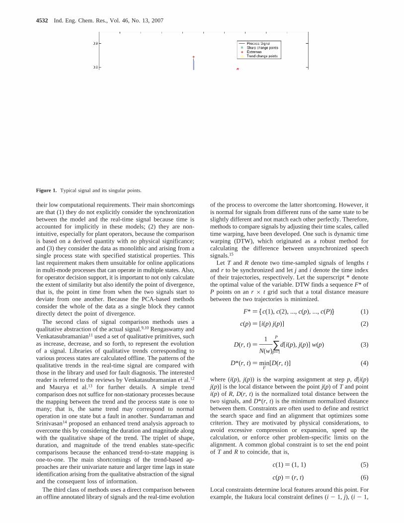
Figure 1. Typical signal and its singular points.

F* ) c(1), c(2), ...,c(p), ...,c(P) (1)

c(p) ) [i(p) j(p)] (2)

D(r, t) )1

N(w)∑p)1

P

d[i(p), j(p)] w(p) (3)

D*( r, t) ) minF

[D(r, t)] (4)

c(1) ) (1, 1) (5)

c(p) ) (r, t) (6)

4532 Ind. Eng. Chem. Res., Vol. 46, No. 13, 2007

j - 1), and (i - 1, j - 2) as the set of predecessors to (i, j) andresults in a local slope in [1/2 2]. Let DA(i, j) be the minimumaccumulated total distance between the two signals from (1, 1)to (i, j). The optimization problem in eq 4 reduces to

whereDA(1, 1) ) d(1, 1) and condition (A*) indicates that thepredecessor of point (i - 1, j) is the point (i - 2, j). Moredetails of DTW can be found in Sankoff and Kruskal.15 Kassidaset al.16 used DTW for synchronizing batch trajectories.

A major shortcoming of DTW is its computational complexity(O(t‚r)) which precludes its use with long signals common inthe process industry. Also, the entire assignment history has tobe stored in memory with the concomitant memory require-ments. Further, in many cases, the minimum distance criterionused in DTW does not guarantee comparison and synchroniza-tion of operationally equivalent points of the signal. Toovercome the above limitations, Srinivasan and Qian1 augmentedtime warping by using landmarks in the signal, called singularpoints. We summarize this approach and related developmentsin section 2. Previous applications of DTW have focused onoffline signal comparison, where the two signals to be comparedare entirely available beforehand. For online state identificationor fault diagnosis, a signal that is evolving in real-time has tobe compared. Also, the reference signal is not known a priori.This results in two challenges: (1) locating the optimumreference signal from a library of signals and the point fromwhich comparison between the two signals should start and (2)performing robust signal comparisons with a computationalrequirement suitable for online use. We address these twochallenges in this paper. In section 3, we propose a flankingstrategy for efficiently identifying the reference signal as well

an anchoring strategy for updating the signal comparison whena new sample becomes available. In section 4, the applicationof the method to state identification in the Tennessee Eastmansimulation and fault diagnosis in a lab-scale distillation columnis reported. Summary and conclusions from this work arepresented in section 5.

2. Singular Points Augmented Time Warping

Information content is not homogenously distributed through-out a signal; rather, the majority of the features of the signalare concentrated in a small number of points. Such points, whichare landmarks in the signal evolution, are called singular points.1

The singular points of a sample signal are shown in Figure 1.Mathematically, each singular point is a tripletTSP ) Γ, Ω,Ψ whereΓ is the time of occurrence of the singular point,Ωis the magnitude of the variable at the singular point, andΨ isits type. Three types of singular points can be differentiatedcorresponding to sharp changes, extrema, and trend changes;thus, singular points are broadly points of local extrema in thevariable and its first and second derivatives. The different typesof singular points are not mutually exclusive, and the same pointcan correspond to more than one type. This is illustrated inFigure 1: P1 is both an extreme point and a sharp change point;similarly, P2 and P4 are trend change points as well as sharpchange points. In such cases, the list of all matching types isnoted. Methods for singular points identification are reportedin Srinivasan and Qian1 and Qian.17

The segment of a signal between adjoining singular points iscalled a singular episode. An episode thus consists of regionsof nearly constant slope, small oscillations, and so forth. Clearly,a signal can be deconstructed into adjoining singular episodes;equivalently, a signal can be described through anordered setof singular points. The representation of a signal by its singularpoints enables its efficient synchronization and comparison withanother signal. This is achieved bylinking the singular pointsor episodes of the two signals using dynamic programming. One

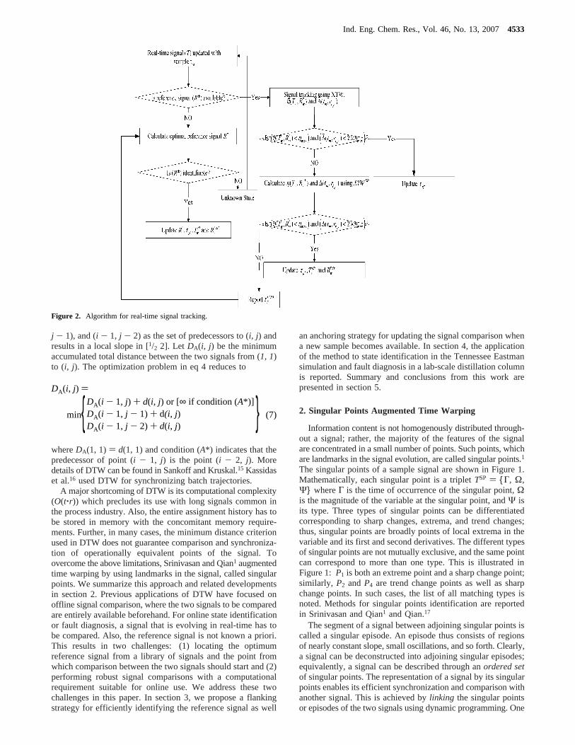
Figure 2. Algorithm for real-time signal tracking.

DA(i, j) )

minDA(i - 1, j) + d(i, j) or [∞ if condition (A*)]DA(i - 1, j - 1) + d(i, j)DA(i - 1, j - 2) + d(i, j) (7)

Ind. Eng. Chem. Res., Vol. 46, No. 13, 20074533

important criterion for linking two sets of singular points is thattheir sequences should match. AsequenceViolation occursbetween a pair of singular points (Tm

SP, RmSP) and (Tk

SP, RlSP) in

signalsT andR if m < k (that is,TmSP temporally precedesTk

SP)

but m > l (that is,RmSP doesnot temporally precedeRl

SP). Asdescribed in detail in Srinivasan and Qian,1 the singular pointsof two signals are said tocorrespondand can be linked if theyare of the same type and if the linkage does not result in anysequence violations. For a given linkage of singular points, thedistance between the two signals is calculated as the sum ofepisode-wise distances. Time warping is used to calculate thedistance between the corresponding episodes so as to accountfor magnitude and duration differences between the episodes.Among the various linkages possible between two singular pointsequences, the linkage that results in minimum signal distanceis considered optimal.

Srinivasan and Qian1 also proposed a new time warpingstrategy called extrapolative time warping (XTW), which is agreedy search modification of classical DTW with Itakura localconstraint. The XTW method obviates dynamic programmingfor each local point by optimizing each point locally. In contrastto DTW, search in XTW proceeds in the forward directionstarting from the first point of the signal to the last. Given thewarping assignment (i, j), the optimal warping for the subsequentstep, that is, the location ofj* that corresponds to (i + 1), isbased only on the previous decision and the current distance.

Figure 3. Algorithm for optimal reference signalR* identification.

Figure 4. Flanking segments used for reference signal identification.


Three possible successors, (i + 1, j), (i + 1, j + 1), and (i + 1,j + 2), are considered. In lieu of eq 7, the optimal search pathin XTW is therefore defined by

with initial condition DA(1, 1) ) d(1, 1). Condition (B*)indicates that the predecessor of pointj* ) j. Thus, for eachstep, the decision for the corresponding point fori is based onlyon three comparisons: to increasej by 0, 1, or 2. Followingthe Itakura local constraint, if the previous decision was toincreasej by 2, then the successor would not have this option(so as to maintain the local slope in the [1/2 2] range), andj canincrease only by 0 or 1. Similarly, in the preceding step, ifjdid not increase, the successor would not have the option toremain at the samej, and j* ) j + 1 or j* ) j + 2. Becauseany decision is based only on the previous decision and thecurrent difference, dynamic programming is obviated. Thesearch space of the XTW is the same as DTW with the Itakuralocal constraint. However, unlike DTW, in XTW once a matchhas been assigned, future assignments will not affect it. Theassignment history tree, which is the origin for the largecomputational storage requirements of DTW, is not necessaryin XTW; instead only the list of assignments needs to bemaintained. The greedy extrapolative search for any pointdecreases the computational time and provides a major advan-tage when XTW is used in online signal tracking as explainedin section 3. However, because global information is not usedat each step, an optimal solution is not guaranteed by XTW.This issue comes to the foreground when long signals have tobe compared. In our approach, this is addressed by combiningXTW with singular point linkage.

The singular points based time warping approaches enforcethe optimal linkage of the major landmarks of the two signals

using dynamic programming. The global optimality of theepisode-level comparison is therefore not a critical requirementbecause the optimal assignment of each time point within anepisode has no physical significance and is rarely necessary inpractical applications. The two-step comparison also leads tosignificant improvements in speed, memory requirement, andefficiency of signal comparison. Another important advantageis that because the singular points have physical meaning suchas the beginning or ending of a process event, they can bedirectly used for state identification, monitoring, and supervision.Singular point augmented time warping is suited for signalswhose endpoints are known to correspond as these are used inthe initial warping assignment (1, 1). This is not the case in

Figure 5. Temporal development and translation of flanking segments during optimal reference signal identification.

DA(i + 1, j*) ) min

DA(i, j) + d(i + 1, j) or [∞ if condition (B*)] j* ) jDA(i, j) + d(i + 1, j + 1) j* ) j + 1DA(i, j) + d(i + 1, j + 2) j* ) j + 2

(8)

Table 1. TE Process Measurements and Their Base Values

variable namevariablenumber

base casevalue units

A feed (stream 1) XMEAS (1) 0.25052 kscmhD feed (stream 2) XMEAS (2) 3664.0 kg h-1

E feed (stream 3) XMEAS (3) 4509.3 kg h-1

A and C feed (stream 4) XMEAS (4) 9.3477 kscmhrecycle flow (stream 8) XMEAS (5) 26.902 kscmhreactor feed rate (stream 6) XMEAS (6) 42.339 kscmhreactor pressure XMEAS (7) 2705.0 kPa gaugereactor level XMEAS (8) 75.0 %reactor temperature XMEAS (9) 120.40 °Cpurge rate (stream 9) XMEAS (10) 0.33712 kscmhproduct separator

temperatureXMEAS (11) 80.109 °C

product separator level XMEAS (12) 50.000 %product separator pressure XMEAS (13) 2633.7 kPa gaugeproduct separator

underflow (stream 10)XMEAS (14) 25.160 m3 h-1

stripper level XMEAS (15) 50.000 %stripper pressure XMEAS (16) 3102.2 kPa gaugestripper underflow

(stream 11)XMEAS (17) 22.949 m3 h-1

stripper temperature XMEAS (18) 65.731 °Cstripper steam flow XMEAS (19) 230.31 kg h-1

compressor work XMEAS (20) 341.43 kWreactor cooling water

outlet temperatureXMEAS (21) 94.599 °C

condenser cooling wateroutlet temperature

XMEAS (22) 77.297 °C


real-time signal comparison where the online signal is availablestarting from an unknown state. We use dynamic locus analysis(DLA) to identify the endpoints in the library signal thatcorrespond to those of the real-time signal.

2.1. Dynamic Locus Analysis for Finding the Best Match-ing Segment.DLA is an efficient method to compare a shortsignal with a long reference signal and identify the best matchingsegment from the reference.2 Consider the short signalX ) x1,x2, x3, ...,xm which is the lastmsamples from an online sensor.Herem is the size of the evaluation window. LetY ) y1, y2,y3, ..., yn be a long reference signal. For every segment ofY,sayZ ) yl, yl+1, ..., yj, a segmentZ* ) yl*, yl*+1, ..., yj*, iscalled thelocusof X if

Also, yl* is called thecorresponding pointof x1, andyj* is thecorresponding point ofxm. The brute force approach ofconsidering each possiblel in Yand performing an independentcomparison will result in an unacceptable computational load.DLA overcomes this by extending Smith and Waterman’s18

dynamic programming approach for comparing protein se-quences. In DLA, the locus ofX is identified by using adissimilarity matrix,DS. Let i and j be the time indices ofXand Y, respectively. The (i, j) element ofDS measures theminimal difference between the sub-segmentx1, x2, x3, ..., xiin X and the sub-segmentyl, yl+1, yl+2, ...,yj in Y. In the generalcase,l is unknown and is determined using dynamic program-ming.

whereyj(d) is the time warped point that matches withxd and∆(xd, yj(d)) ) |yj(d) - xd| is the difference betweenxd andyj(d).Because the optimal search should allow for compression andelongation inY relative toX, time warping is used to synchronizeX andY. Following DTW with Itakura local constraint, eq 10reduces to

whereG* indicates that the predecessor of point (i - 1, j) isthe point (i - 2, j). Note thatDS(i, j) is not the total minimumdistance betweenx1, x2, x3, ..., xi andy1, y2, ..., yj, rather itis the total minimum distance betweenX and its locus inY.Segments ofY that are similar toX would lead to small valuesof DS. The optimal match betweenX and the locus inY is givenby DS(m, j*) where j* ) argminjDS(m, j) j ∈ [1 n]. Moredetails of DLA can be found in Srinivasan and Qian.2 In thispaper, we extend DLA and singular point augmented timewarping for online signal comparison.

3. Online Signal Comparison Using Singular PointsAugmented Time Warping

The online signal comparison problem can be stated asfollows: Given a set of reference signalsK and a real-time signalT emanating from the process operating at an unknown state,(1) identify the reference signal that best matches the currentstate of the process and (2) identify the progress of the process

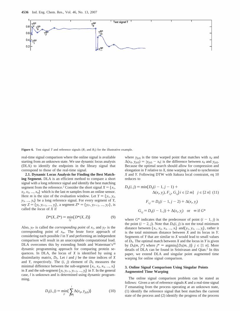
Figure 6. Test signalT and reference signals (R1 andR2) for the illustrative example.

D*(X, Z*) ) minl,j

D*(X, Z) (9)

DS(i, j) ) minF

∑d)1

i

∆(xd, yj(d)) (10)

DS(i, j) ) minDS(i - 1, j - 1) +∆(xi, yj), Fi,j, Gi,ji ∈ [2 m] j ∈ [2 n] (11)

Fi,j ) DS(i - 1, j - 2) + ∆(xi, yj)

Gi,j ) DS(i - 1, j) + ∆(xi, yj) or ∞ if G*


with respect to the reference signal. The former is called theoptimal reference signal identification problemwhile the latteris referred to asreal-time signal (or state) tracking. The firststep involves comparison of the real-time signal with manyreference signals and is computationally more intensive thanthe second step; hence, although the first step could be repeatedat every instant, it is not tenable for online application, wherethe requirement is that the calculation time at every sample mustbe less than the sampling interval∆τ. New signal comparisonstrategies that extend XTWSP and DLA are needed for thesepurposes.

3.1. Flanking Strategy for DLA. The DLA provides anefficient way to identify the locus: a sub-segment of a longsignal that best matches another (short) signal. Although DLAcan be directly used for optimal reference signal identification,because its computational cost is proportional to the length ofthe two signals (real-time and reference), its efficiency wouldcontinually decrease as the real-time signal evolves and becomeslonger. The flanking strategy bounds the length of the signalused for locus identification by decomposing the real-timesignal.Flanking segments, signal segments of fixed length fromthe beginning and end of the signal, are used for this purpose.Consider a signalX ) x1, x2, ..., xm, wherem g 2ν. In theflanking strategy,X is decomposed into three segments: theanterior flanking segment, the core segment, and the posteriorflanking segment. Theanterior flanking segmentof X is defined

as its firstν points, that is,XA ) x1, x2, ..., xν whereν is theflank length. Similarly, theposterior flanking segmentof X isdefined as the lastν points, that is,XP ) xm-ν+1, xm-ν+2, ...,xm. The innerm - 2ν points ofX comprise thecore segmentas illustrated in Figure 4 for a sample signal.

The flanking segments of the signal can be used to identifythe locus ofX efficiently based on the recognition that any lociiof X should also have segments that have high similarity withthe flanking segmentsXA andXP. The flanking strategy exploitsthis property. Given a long reference signalY, all the segmentsin Y, sayYA, that closely matchXA can be identified. Similarly,all adequate matches forXP, sayYP, can also be identified. Notethat the lengths ofYA and YP may not be equal to the flanklength due to run-to-run variations between the real-time andthe reference signals. Each pair ofYA andYP whereYA precedesYP in Y can be used to construct a uniquecomposite segment Zsandwiched byYA andYP, Z ⊂ Y. Each composite segment isa possible locus ofX. By eq 9, the locus ofX in Y is thecomposite segmentZ* which has the least difference withT.The flanking strategy is thus a generalization of the DLA foridentifying the locus of a longer signal. It recognizes that thecomputational complexity of any signal comparison methoddepends directly on the length of the two signals to be compared.The flanking strategy is computational efficient because the twoflanking segments are short; therefore, the cost of the first phaseof comparisons with all the reference signals is small and

Figure 7. Comparison of real-time signalT at τT ) 8 with R1 (shown in part b) reveals a minimum atτR1 ) 199 (shown in part c). Similar comparison withR2 depicted in part d shows a minimum atτR2 ) 1083 as shown in part e.


bounded byν. In general, any method can be used to identifythe locii YA andYP; we use DLA as described in section 3.4.Also, any method can be used to compare the compositesegmentsZ with X; we use XTWSP for this purpose.

3.2. Anchoring Strategy for Time Warping. The anchoringstrategy also seeks to improve the computational efficiency of

comparing a signal that is evolving in time. ConsiderX ) x1,x2, x3, ..., xm, the lastm samples from an online sensor, andY) y1, y2, y3, ..., yn, a long reference signal. Let a segment ofY, sayy1, ..., yj be known to matchx1, x2, x3, ..., xm. Thebase pointat time m is defined as the point in theY thatcorresponds toxm. In this case, the base point at timem is yj.

Figure 8. Snapshot atτT ) 226 of signal comparison betweenT andR.

Figure 9. Snapshot atτT ) 682 of signal comparison betweenT andR.


The portion ofX used for comparison is called theeValuationwindowand notated by the subscript w. The matching segmentin Y is also notated by the subscript w. Thus, if the entireX isused for comparison,Xw ) x1, ..., xm andYw* ) yl, ..., yj.When a new samplexm+1 becomes available from the onlinesensor,Xw is extended by appendingxm+1, and the base pointhas to be recalculated. Any time warping method can be usedfor this purpose. As mentioned above, the computational expenseof signal comparison increases with signal length; therefore, asnew samples are obtained, it takes ever-increasing time tocalculate the base point because the evaluation window increasesmonotonically.

The anchoring strategy provides a systematic way of trimmingthe evaluation window without sacrificing accuracy. It relieson the insight that the entireX does not need to be comparedwith Y at every instant. If at timem, x1, ..., xm has matchedy1, ..., yj, then any future divergence ofX from Y can bedetected using only recent observations ofX in the evaluationwindow.

Anchor pointsare 2-tuples fromX andY that are known tocorrespond. In the above, (x1, y1) can be considered an anchorpoint. In general, any pair of singular points inX and Y, sayXSP andYSP, that have been linked by dynamic programmingcan be used as anchor points. Also, iftXSP andtYSP are the timesof occurrence ofXSP and YSP, respectively, then two non-overlapping segments can be differentiated inX comprising the

observationsx1, ..., xtXSP-1 before the anchor point and the

ones after,xtXSP, ..., xm. Similarly, Y is split by the anchor

point into two segments:y1, ..., ytYSP-1 and ytX

SP, ..., yn.Denoting the difference betweenX andY by ∆(X, Y),

Using the linear additivity property,

BecauseXSP and YSP are linked singular points,∆(x1, ...,xtX

SP-1, y1, ..., ytYSP-1) ≈ 0 and∆(X, Y) ≈ ∆(xtX

SP, ..., xm,ytX

SP, ..., yn). So, for updating the base point, the evaluationwindow can be shortened to begin from the anchor point,Xw )xtX

SP, ...,xm andYw* ) ytXSP, ...,yj. The proposed online signal

comparison approach uses the anchoring and flanking strategiesfor real-time signal tracking and optimal reference signalidentification sub-problems as described next.

3.3. Real-Time Signal Tracking Using Anchoring Strategy.This step uses the optimal reference signalR* calculated a priori(see section 3.4) and seeks to confirm that the process continuesto operate in the same state (i.e., same reference signal). It thuscalls only for resynchronization of the real-time signalT basedon the additional sample withR*. In the following, for ease of

Figure 10. Comparison of real-time signalT at τT ) 685 with R1 (shown in part b) reveals a minima atτR1 ) 185 (shown in part c). Similar comparisonwith R2 depicted in part d shows a minimum atτR2 ) 1087 as shown in part e.

∆(X, Y) ) ∆(x1, ...,xm, y1, ...,yj) (12)

∆(X, Y) ) ∆(x1, ...,xtXSP-1, y1, ...,ytYSP-1) +

∆(xtXSP, ...,xm, ytXSP, ...,yn) (13)


explanation, the time variable for the real-time signal is denotedasτT and that of reference signalR asτR. The two signals canbe compared starting from the beginning (i.e.,τT ) 1);alternatively a smaller evaluation window can be used on thebasis of the anchoring strategy described above. We pursue thelatter option for computational efficiency purposes.

Consider the real-time signalT ) t1, ..., ti, ..., tm-1. Theevaluation window is defined as per the anchoring strategy based

on singular points. Let the last singular point inT be at timeτT

) τTSP and let the value ofT at that time bettTSP. The

corresponding singular point inR* can be obtained usingXTWSP. These singular points inT andR* for the anchor pointof the evaluation window. So, the evaluation windowTw at τT

) m - 1 is Tw ) ttTSP, ttTSP+1, ..., tm-1. Let the correspondingsegment ofR* that matchesTw be Rw

/ . When a new sampletmbecomes available atτT ) m, Tw is updated, and the task in

Figure 11. Schematic of the Tennessee Eastman19 process with control system.

Table 2. Disturbance Profiles for TE Process (a) XD1 (b) XD2 (c) XD3 (d) XD4 (e) XD5.

targettime(min) target

time(min) target

time(min) target

time(min)

(a) XD1XD1-A 1.20‚base value 180 1.40‚base value 190 1.60‚base value 200 1.0‚base value 780XD1-B 1.15‚base value 240 1.35‚base value 254 1.55‚base value 268 1.0‚base value 900XD1-C 1.10‚base value 300 1.30‚base value 318 1.50‚base value 336 1.0‚base value 1020

(b) XD2XD2-A 1.03‚base value 180 1.05‚base value 190 1.07‚base value 200 1.0‚base value 1020XD2-B 1.025‚base value 240 1.045‚base value 254 1.065‚base value 268 1.0‚base value 1080XD2-C 1.02‚base value 300 1.04‚base value 318 1.06‚base value 336 1.0‚base value 1200

(c) XD3XD3-A 1.05‚base value 180 1.10‚base value 190 1.15‚base value 200 1.0‚base value 780XD3-B 1.045‚base value 240 1.09‚base value 254 1.135‚base value 268 1.0‚base value 900XD3-C 1.04‚base value 300 1.08‚base value 318 1.12‚base value 336 1.0‚base value 1020

(d) XD4XD3-A 1.05‚base value 180 1.10‚base value 190 1.15‚base value 200 1.0‚base value 780XD3-B 1.045‚base value 240 1.09‚base value 254 1.135‚base value 268 1.0‚base value 900XD3-C 1.04‚base value 300 1.08‚base value 318 1.12‚base value 336 1.0‚base value 1020

(e) XD5XD5-A 0.95‚base value 180 0.90‚base value 190 0.85‚base value 200 1.0‚base value 780XD5-B 0.955‚base value 240 0.91‚base value 254 0.865‚base value 268 1.0‚base value 900XD5-C 0.96‚base value 300 0.92‚base value 318 0.88‚base value 336 1.0‚base value 1020


real-time signal tracking is to update the base point andRw/

through resynchronization as well as confirm thatRw/ continues

to matchTw. In our approach, this is achieved in two steps, asshown in Figure 2:

Step A: Efficient Calculation of the Difference betweenthe Real-Time Signal and the Reference Signal.Any signalcomparison method can be used for calculating the differencebetweenTw andRw

/ . We use XTW for this purpose because ofits advantageous time and space requirements. The normalizedtime-warped distance betweenTw and Rw

/ is calculated asfollows:

The numerator is the XTW difference betweenTw and Rw/

while the denominator is the length of the evaluation window.The difference between the latest real-time sampletm and itswarping assignment inR* as per XTW, notated as∆(tm, rτR*),is also calculated. If

is satisfied, the process is considered to continue in the samestage of operation, and only the base pointτR* is updated. Thefirst condition ensures that the broad overall trend of thereference and real-time signals is the same while the secondcondition allows for larger local variations in the signal due tonoise or run-to-run differences. The computational efficiency

of XTW comes at a price: a largeη(Tw, Rw/ ) does not

guarantee thatTw is dissimilar from Rw/ because the local

greedy search in XTW can lead to an overestimate of thedifference when signals become long.1 Such artifacts can beeliminated by a more accurate calculation using XTWSP, whennecessary.

Step B: Accurate Calculation of the Difference betweenthe Real-Time Signal and the Reference Signal.XTWSPlinksthe singular points in the real-time and reference signals andthus calculates an accurate difference betweenTw andRw

/ . Soif eq 15 is not satisfied, a more accurate difference is calculatedusing XTWSP, and a condition analogous to eq 15 is evaluatedto confirm divergence ofT from R*.

Here,η(Tw, Rw/ ) is the difference betweenTw andRw

/ while ∆-(tm, rτR*) is the distance betweentm and the base point ascalculated using XTWSP. Note thatη(Tw, Rw

/ ) e η(Tw, Rw/ )

because XTWSP relies on singular point linkage. If eq 16 issatisfied, the process is considered to continue in the same state(i.e., no change to the reference signal), and the base point isupdated. One byproduct of performing XTWSP is that newsingular points could have been identified inTw and linked withR*. The last singular point inT and its corresponding linkedsingular point inR* are subsequently used as the new anchorpoint which results in the shortening of the evaluation window.So, future Step A and Step B calculations become more efficientand accurate. If condition 16 is not satisfied, the process isconsidered to have moved to a new state, and another optimal

Figure 12. Three runs of XD1 in the TE case study with different magnitudes and duration.

η(Tw, Rw/ ) )

∑i)τT

SP

m

|rj(i) - ti|

m - τTSP+ 1

(14)

(η(Tw, Rw/ ) < ηmax) and (∆(tm, rτR*

) < 2 × ηmax) (15)

(η(Tw, Rw/ ) < ηmax) and (∆(tm, rτR*

) < 2 × ηmax) (16)


reference signal has to be identified, starting atτT ) m as thepoint of divergenceτT

POD.3.4. Optimal Reference Signal Identification.The task in

this stage is to identify the reference signalR* that best matchesthe state of the process at timetm. This would be required atτT

) 1 when the reference signal is not known and when the real-time signal has diverged from the previous reference (i.e., eq16 is not satisfied). Consider adiVergent segmentof T rangingfrom the point of divergence to the latest sample:

Note thatτTPOD ) 1 atτT ) 1. The process state is identified by

comparing the divergent segment with all the reference signalsin the library (K). Consider a reference signalR ) r1, r2, r3,..., rn from K with time indexj. Let η(TD, R) be the normalizeddifference betweenTD andR. The optimal reference signalR*is defined as

A tradeoff exists between the speed and accuracy of referencesignal identification. If the divergent segment used for identify-

ing R* is small, several good matches may exist inK. Wequantify the accuracy of the located optimal reference signal interms of theinseparability ratioR, defined as the ratio of thenormalized difference of the best matching reference signal tothat of the second-best one:2

The inseparability ratio thus reflects the uniqueness ofR*.Following Srinivasan and Qian,2 the criterion for the optimalreference signal atτT ) m with base pointτR* is

where the first condition ensures low difference betweenTD

andR* while the latter ensures its uniqueness. If eq 20 is notsatisfied atτT ) m, an unknown state is flagged, and thecalculation ofR* and τR* is repeated when the next real-timesample becomes available atτT ) m + 1.

Next, we describe how the differenceη(TD, R) is calculated.Because the suitable start and endpoints ofTD in R are notknowna priori, the locus ofTD in R has to be first calculated.The DLA can be used for this purpose but as described in section

Figure 13. Schematic of the lab-scale distillation column.

TD ) tτT

POD, ..., tm if m g τTPOD + ν

tm-ν+1, ..., tm if ν e m < τTPOD + ν

(17)

R* ) arg minR∈K

(η(TD, R)) (18)

R )η(TD, R*)

minR∈K,R*R*

(η(TD, R))(19)

(η(TD, R*) < ηmax) and (R < Rmax) (20)


3.1 it is efficient as long as the length of the divergent segmentis small. The flanking strategy proposed earlier becomesnecessary if the divergent segment becomes long. We thereforeconsider two different phases as shown in Figure 3.

En Bloc Comparison Phase.When the divergent segmentis small, that is,m - τT

POD < 2ν, and can be used in its entirety,DLA is directly used to identify the locus of the divergentsegment. The normalized difference is calculated as

where (i, j) is the warping assignment betweenTD and its locusin R. As mentioned above, if eq 20 is not satisfied and theoptimal reference signal cannot be clearly determined, com-parison is repeated when the next real-time sample becomesavailable. Thus the length of the divergent segment wouldincrease with time. Once the length ofTD becomes large, DLAbecomes computationally expensive. We minimize the compu-tational requirement for such cases using the flanking-basedcomparison strategy.

Flanking Phase.When the divergent segment is large,m -τT

POD g 2ν and the flanking strategy becomes necessary. Shortflanking segments from the start and end ofTD provide the basisfor identifying the locus ofTD in R. The anterior flankingsegment of the divergent segment isXA ) tτT

POD, tτTPOD+1, ...,

tτTPOD+ν-1 and the posterior flanking segment isXP ) tm-V+1,

tm-ν+2, ..., tm; thus,TD is sandwiched by the flanking segments.

DLA is used to identify all the matching segmentsYA in Rsuch thatη(XA, YA) < ηmax. [One significant point needs to benoted here. In contrast to the original DLA where only the bestmatching segment is identified, here several candidate segmentsmay be identified. To optimize the calculation, candidates thatare not at least one singular point away from a better candidate(in terms of smallerη) are rejected, so as to yield a well-separated set of candidate segments (see Qian17).] The samecriterion is applied to obtain all reference signal segmentsYP

that matchXP. Each pair ofYA and YP defines a differentcomposite segment inR. Because in general these compositesegments can be long, XTWSPis used to synchronize them withTD. The difference betweenTD and R is then calculated asfollows:

Figure 5 shows how the en bloc comparison and the flankingphase are integrated in the proposed method for reference signalidentification. When the process moves away from the previousstate as indicated by eq 16, the immediately precedingν pointstτT-ν+1, ..., tτT are used as the divergent segment and en bloccomparison performed to identify the reference signal. If theoptimal reference signal, as per eq 20, cannot be identified byτT ) τT

POD + 2ν the divergent segment is split into anterior andposterior flanking segments, each of lengthν, and the flanking

Figure 14. Process signals from Run-03 of the lab-scale distillation column.

η(TD, R) )

∑i)m-ν+1

m

|rj(i) - ti|

ν(21)

η(TD, R) )

∑i)τT

POD

m

|rj(i) - ti|

m - τTPOD + 1

(22)


strategy is used. In this flanking phase of reference identification,only the posterior flank is translated when a new sample is addedto the divergent segment. The anterior flanking segment remainsanchored atXA ) tτT

POD, tτTPOD+1, ..., tτT

POD+ν-1. The length ofthe divergent real-time signal increases with time; however, theoptimal reference identification is calculated in a computation-ally efficient fashion suited for online use. A detailed illustrationis given next to explain the above-described signal comparisonalgorithm.

3.5. Illustrative Example. Consider the test signalT and thetwo reference signalsR1 andR2 shown in Figure 6. Online datahave been collected starting atτT ) 1. Because the optimalreference signal is unknown initially, it has to be identified firstfollowing the description in section 3.2.τT

POD ) 1, and signalcomparison starts atτT ) 8 () ν). The en bloc differencecalculation strategy is first used for finding the locus in referencesignalsR1 andR2 since the signal length atτT ) 8 is less than2ν. At τT ) 8, the DLA difference forR1 andR2 are as shownin Figure 7.DS(ν, τR1) has a clear minimum atτR1 ) 199 andη(T, R1) ) 0.0151 (<ηmax ) 0.05). The locus for the divergentsegment inR2 is atτR2 ) 1083 andη(T, R2) ) 0.0836 (> ηmax).Therefore,R ) 0.1810 (< Rmax ) 0.70). So atτT ) 8, R1 isconfirmed to be the optimal reference signal withτR1 ) 199 asthe base point. From the next sample,τT ) 9, real-time signaltracking as described in section 3.3 is performed to confirmthat T progresses as per reference signalR1.

A snapshot of the real-time signal tracking atτT ) 226 isshown in Figure 8. At this time, the anchor for comparisonbetweenT andR1 is the previous corresponding singular pointswith τT

SP ) 164 andτR1

SP ) 359. The base point is atτR1 ) 413.

Therefore, the evaluation windowTw ) t164, ..., t226 iscompared withRw

/ ) r359, ..., r413 using XTW. η(Tw, Rw/ ) )

0.0180 (< ηmax) and ∆(tm, rτR*) ) 0.0086 (<2 × ηmax), socondition 14 holds and tracking can continue. Online trackingproceeds similarly untilτT ) 682 whenη(Tw, Rw

/ ) ) 0.0217,but ∆(tm, rτR*) ) 0.3666 (>2 × ηmax), so eq 15 is violated.XTWSP is then used for accurate calculation of the differencebetweenTw and Rw

/ . η(Tw, Rw/ ) ) 0.0213 and∆(tm, rτR*) )

0.3633 (>2 × ηmax), so eq 16 is violated too. This confirmsthat the real-time signal is no longer similar toR1 and thereference signal has to be re-identified withτT

POD ) 682 (seeFigure 9).

The divergent segmentTD ) t675, t676, ..., t682 is used tofind the new reference signal through DLA. Initially,m - τT

POD

< 2ν, so en bloc difference calculation is performed. AtτT )682,η(TD, R2) ) 0.0641,R ) 0.9596, and eq 20 does not hold,so the reference signal cannot be conclusively identified.Comparison is therefore repeated when subsequent samplesbecomes available. As shown in Figure 10, atτT ) 685,η(TD,R2) ) 0.0388 (< ηmax), andR ) 0.6039 (< Rmax). So the newreference signal is confirmed to beR2 with τR2 ) 1082 as theanchor point andτR* ) 1087 as the base point.

In the next section, we evaluate the proposed online signalcomparison on two case studies.

4. Case Studies

4.1. Case Study 1: Online Disturbance Identification inthe Tennessee Eastman Process.The Tennessee Eastman (TE)process19 is a popular test bed for process control, faultdiagnosis, and signal comparison. In this section, data from thissimulated plant are used to test the accuracy of the proposedmethod. The TE process produces two products (G and H) anda byproduct (F) from reactants A, C, D, and E. The processflowsheet is shown in Figure 11. The process has five units: atwo-phase reactor, a product condenser, a flash separator, arecycle compressor, and a product stripper. There are 53variables in the TE plant: 22 of these are process measurementvariables, 19 are component compositions, and 12 are process-manipulated variables. The closed-loop process simulator usedhere was developed by Singhal20 on the basis of the base controlstructure of McAvoy and Ye.21 During the simulation, variablevalues are recorded every minute. The 22 process measurementsused in this paper for process state identification are shown inTable 1.

In this case, we use dynamic signal matching to identifyprocess disturbances online. Five disturbance classes, calledXD1-XD5, that affect the A feed flowrate, reactor pressure,reactor level, reactor temperature, and compressor work are

Table 3. Offline Signal Difference between Different Disturbance Instances in the TE Process Using Direct Comparison (×10-1)

XD1-A XD1-B XD1-C XD2-A XD2-B XD2-C XD3-A XD3-B XD3-C XD4-A XD4-B XD4-C XD5-A XD5-B XD5-C

XD1-A 0 0.0686 0.074 0.2228 0.2052 0.1983 0.1735 0.1647 0.161 0.3631 0.3589 0.3443 0.0977 0.1108 0.1054XD1-B 0 0.0629 0.2235 0.2028 0.1953 0.1735 0.1564 0.1476 0.3739 0.3483 0.3387 0.1136 0.0903 0.1023XD1-C 0 0.2241 0.2009 0.1885 0.1847 0.1587 0.1383 0.3694 0.357 0.3278 0.1114 0.1018 0.0824XD2-A 0 0.1446 0.166 0.2327 0.2309 0.1892 0.4558 0.4544 0.4107 0.2004 0.2015 0.1739XD2-B 0 0.11 0.2631 0.2342 0.2413 0.4555 0.4219 0.4247 0.1914 0.1791 0.1801XD2-C 0 0.2465 0.2424 0.2157 0.4556 0.4351 0.4001 0.1875 0.1786 0.1624XD3-A 0 0.1991 0.1816 0.4143 0.4318 0.4113 0.1591 0.1718 0.1626XD3-B 0 0.1736 0.4482 0.3953 0.4007 0.176 0.1415 0.1565XD3-C 0 0.4294 0.4175 0.3697 0.1681 0.1521 0.124XD4-A 0 0.2139 0.2909 0.3386 0.3605 0.3812XD4-B 0 0.2003 0.3616 0.3262 0.3425XD4-C 0 0.3589 0.337 0.3063XD5-A 0 0.1005 0.0868XD5-B 0 0.0864XD5-C 0

Table 4. Disturbance Identification during Run-4 of the TE CaseStudy

η

τT R1 R3 R4 R5 R

1030 0.0501 0.0511 0.0514 0.0512 0.98041031 0.0592 0.0593 0.0589 0.0581 0.98641032 0.0659 0.0656 0.0654 0.0647 0.99701033 0.0693 0.0654 0.0572 0.0683 0.87461034 0.0723 0.0604 0.0408 0.0702 0.67551035 0.0755 0.0556 0.0240 0.0723 0.43171036 0.0782 0.0510 0.0072 0.0742 0.14121037 0.0779 0.0506 0.0070 0.0739 0.13831038 0.0773 0.0508 0.0068 0.0732 0.13391039 0.0767 0.0507 0.0065 0.0729 0.12821040 0.0760 0.0506 0.0064 0.0723 0.12651041 0.0752 0.0504 0.0061 0.0716 0.12101042 0.0745 0.0500 0.0061 0.0712 0.12201043 0.0737 0.0505 0.0060 0.0707 0.11881044 0.0729 0.0504 0.0060 0.0703 0.1190


studied here (see Table 2). Different instances (runs) of the samedisturbance class have different start times, duration, andmagnitude. For example, during XD1-A, the flowrate of A feedfrom upstream is increased from the base case value of 0.25052kscmh to 0.3902 kscmh (a 60% change) in three steps startingat t ) 180 min as shown in Table 2a. After the process recoversfrom these, the inverse change, decreasing the A feed flow, isintroduced att ) 780 min. The process is then allowed to returnto a steady state. The effect on the A flow rate (XMEAS(1))and the downstream pressures (XMEAS(13) and XMEAS (16))is shown in Figure 12. Two other instances XD1-B and XD1-Cwith changes of magnitude of 55% and 50% were alsointroduced. As described in Srinivasan et al.8 similar changeswere introduced to bring forth the other disturbance classes.One instance from each of the classes, XD1-B, XD2-B, XD3-B, XD4-B, and XD5-B, was used to develop the referencedisturbance database for online disturbance identification.

The difficulty in identifying the disturbance online can beestimated by a preliminary analysis. Table 3 shows the differ-ence between the 15 disturbances calculated as the averagedifference among signals. Comparison is made after signals havebeen normalized to [0 1] on the basis of the range of the sensor(see Srinivasan et al.8). As can be seen from the table, theminimum inter-class distance is 0.0824 (between XD1-C andXD5-C) and the maximum intra-class distance is 0.2909 (classXD4). Therefore, difference between the classes by directcomparison, even if the complete signal is available, is anontrivial exercise. In this work, we consider the even moredifficult task of differentiating between the disturbances as theyevolve.

The proposed online signal comparison method is used foronline disturbance identification as follows. Consider Run-4where the process is in state XD2 untilτT ) 1030. An unknowndisturbance occurs starting atτT ) 1030 which is initially

indicated whenη(Tw, Rw/ ) ) 0.0028,∆(tm, rτR*) ) 0.3147, and

eq 14 is violated. An accurate difference is calculated usingXTWSP and η(Tw, Rw

/ ) ) 0.0022 and∆(tm, rτR*) ) 0.3065.Because this is larger than the 2× ηmax threshold even afterresynchronization, as per eq 15 it is evident that the real-timesignal does not confirm to reference signalR2 starting fromτT

) 1030 () point of divergenceτTPOD). The disturbance can be

identified by calculating the new optimal reference signalR*and the base pointτR* using the divergent segmentTD ) tm-V+1,tm-ν+2, ..., tm. In the first iteration, at timeτT ) 1030,η(T, R1)) 0.0501,η(T, R3) ) 0.0511,η(T, R4) ) 0.0514, andη(T, R5)) 0.0512 (see Table 4). Because theη values for all thereference signals are similar (as indicated by the inseparabilityratio R ) 0.9804> Rmax), R* cannot be identified at this pointand further iterations are necessary. In each subsequent iteration,as the real-time signalT evolves, the evaluation window isupdated (as shown in Figure 5) and the analysis repeated. Asthe disturbance becomes more evident with time,R decreases(see Table 4), and atτT ) 1034,η(T, R4) falls belowηmax. Theoptimal referenceR* is then identified asR4 (i.e., disturbanceXD4). The base point atτR* ) 314 inR4 is found to correspondto τT ) 1034. Real-time signal tracking is then resumed forsubsequent samples. The average time cost for this run was0.0273 CPU seconds with the proposed method as against55.2721 CPU seconds with DTW as summarized in Table 5(depicted as the second disturbance in Run-4). This brings outthe computational advantages of the proposed strategy.

Similar disturbance identification studies were performed for14 other runs. Details of these are presented in Qian17 and onlya summary is presented here. Similar high accuracies were foundin all test runs as shown in Table 5. In each run, two disturbanceswere introduced. In all cases, the proposed method correctlyidentified the disturbance with an average delay of 5.23 min.

Table 5. Online Process Disturbance Detection in the TE Process

disturbanceintroduction

time

disturbanceidentifica-

tiontime

best-matchingreference

identifica-tion

delay(sample)

seconddisturbanceintroduction

time

disturbanceidentifica-

tiontime

best-matchingreference

identifica-tion

delay(sample)

averagetimecost

(CPU s)

averagetime costof DTW(CPU s)

Run-1 9 15 XD1 6 1020 1025 XD4 5 0.0501 55.3446Run-2 9 13 XD1 4 670 675 XD4 5 0.0699 55.2385Run-3 9 13 XD1 4 680 684 XD4 4 0.1233 55.2589Run-4 9 17 XD2 8 1030 1034 XD4 4 0.0273 55.2721Run-5 9 13 XD2 4 1100 1107 XD5 7 0.0734 55.3044Run-6 9 16 XD2 7 420 427 XD5 7 0.1289 55.3314Run-7 9 16 XD3 7 860 867 XD1 7 0.0367 55.3578Run-8 9 13 XD3 4 970 974 XD1 4 0.0689 55.3446Run-9 9 13 XD3 4 1100 1105 XD1 5 0.2509 55.3374Run-10 9 14 XD4 5 820 825 XD2 5 0.0373 55.2985Run-11 9 13 XD4 4 380 387 XD2 7 0.0535 55.3051Run-12 9 17 XD4 8 400 407 XD2 7 0.2024 55.2517Run-13 9 13 XD5 4 500 505 XD3 5 0.0784 55.2919Run-14 9 13 XD5 4 600 604 XD3 4 0.0712 55.3051Run-15 9 13 XD5 4 1080 1084 XD3 4 0.2115 55.2517average 5.1333 5.3333 0.0989 55.2996

Table 6. Standard Operating Procedure (SOP) for Lab-ScaleDistillation Column Startup

distillation column startup SOP

1. set all controllers to manual2. fill reboiler with liquid bottom product3. open reflux valve and operate the column on full reflux4. establish cooling water flow to condenser5. start the reboiler heating coil power6. wait for all of the temperatures to stabilize7. start feed pump8. activate reflux control and set reflux ratio9. open bottom valve to collect product10. wait for all the temperatures to stabilize

Table 7. Process Disturbances During Distillation ColumnOperation

case disturbance type

DST01 reboiler power low stepDST02 reboiler power high stepDST03 feed pump high stepDST04 feed pump low stepDST05 Tray temperature sensor T6 fault random variationDST06 reflux ratio high stepDST07 reflux ratio low stepDST08 bottom valve stickingDST09 cooling water slow driftDST10 low cooling water flow and

feed pump malfunctionstep


The average time cost for online signal comparison is only0.0989 CPU seconds (on a Pentium IV, 2.4 GHz cpu) in contrastto 55.3 s for DTW. This factor of 559 speedup in computationover DTW clearly shows the efficiency of the proposed methodand illustrates its suitability for large-scale applications.

4.2. Case Study 2: Online Fault Diagnosis during Startupof a Lab-Scale Distillation Column. In this section, theproposed methodology is illustrated on a lab-scale distillationunit. The schematic of the unit is shown in Figure 13. Thedistillation column is of 2 m height and 20 cm inner-diameterand has 10 trays. The feed enters at tray 4. The system is wellintegrated with a control console and data acquisition system.A total of 19 variables comprising all tray temperatures, reboilerand condenser temperatures, reflux ratio, top and bottom columntemperatures, feed pump power, reboiler heat duty, and coolingwater inlet and outlet temperatures are measured at 10-sintervals. Cold startup of the distillation column with anethanol-water 30% (v/v) mixture is performed following thestandard operating procedure shown in Table 6. The feed passesthrough a heat exchanger before being fed to the column. Thestartup normally takes 2 h, and different faults such as sensorfault, failure to open pump, too high a reflux ratio, and so forthcan be introduced at different states of operation. The referencedatabase is first populated using data from 11 runs of theprocess: one normal startup and the 10 faults summarized inTable 7.

The online signal comparison algorithm was then used forfault diagnosis and decision support during subsequent startupsof the column. Consider one run (Run-3; Figure 14) when afault was introduced atτT ) 3590 s when the operatorsintroduced too large a feed pump flowrate (200 rpm) to thecolumn. This causes instability in the column resulting in adrastic drop in the column’s temperatures. Results from thisrun show that the real-time signal is initially close to normal.

The difference between the real-time signal and all otherreferences is much higher;R ) 0.2235 atτT ) 6. Starting fromt ) 3700 s, the difference between the real-time signal and thenormal reference increases, indicating that there is a fault duringthe startup operation. The differenceη between the real-timesignal and DST03 is less thanηmax (0.05). Also, theR fallsbelow Rmax (0.70), so the fault is identified as DST03.

Similar tests were done for all other cases. In the interest ofspace, only a summary of the findings is presented in Table 8.Faults in all the test runs were correctly identified with anaverage delay of 3.6 samples (and maximum detection delayof 11 samples for Run-03). All faults could be accuratelyidentified within an average of 5.4 samples of their occurrence.The maximum identification delay was about 12 samples forRun-03. The averageR at the time of identification is 0.3828against theRmax threshold of 0.7, which shows the clearidentification of the faults. The average computation time costat each sample was 0.0594 s, which is much less than thesampling rate of 10 s. The proposed method is therefore clearlysuitable for online fault diagnosis in this case as well.

4.3. Robustness and Parameter Tuning.In this section, therobustness of the proposed online signal comparison method isstudied. Varying amount of noise levels were added to the onlinesignal to investigate robustness to noise. The affect of the tuningparameter settings on online signal comparison was also studied.The interested reader is referred to Srinivasan and Qian1,2 forrobustness studies of singular point detection and DLA.

The robustness of the proposed method to sensor noise isreported in this part using data from the lab-scale distillationcolumn case study. Additional measurement noises ranging from1% to 5% were added to all the original signals and faultdiagnosis performed. The results are shown in Table 9. As hasto be expected, there is an increase in the fault identificationdelay with increasing noise; however, the effect is minimal withthe average delay increasing from 5.3 samples to 6.6 samples.A similar study was performed for the TE case study as well(see Table 10), and the average identification delay increasedfrom 5.1333 samples to 17.7333 samples at 5% noise level.This larger variation in the TE case arises from the inherentcomplexity and larger noise levels in the base process. Overall,the proposed method online signal comparison method is robustto noise.

The proposed method uses two tunable parameters:Rmax andηmax. While in the general case different process signals mayrequire different values of these parameters, we have found thatthe same parameter settings can be used across variables andcase studies. The results of decreasingRmax from 0.80 to 0.60for the distillation column as well as the TE case studies showthat Rmax has no significant affect on fault detection delay. Asmaller Rmax would require a clearer separation between the

Table 8. Faults Diagnosis Results for Lab-scale Distillation Column Case Study

case

time faultintroduced(sample)

detectiontime

(sample)

detectiondelay

(sample)

identificationtime

(sample)τy

(sample)

bestmatchingreference η R

identificationdelay (sample)

time cost(s)

Run-01 1 6 5 6 6 DST01 0.0162 0.2817 5 0.1716Run-02 1 6 5 6 6 DST02 0.0097 0.1091 5 0.1028Run-03 359 370 11 371 13 DST03 0.0101 0.3456 12 0.0317Run-04 356 357 1 360 5 DST04 0.0217 0.6663 4 0.0342Run-05 425 426 1 430 6 DST05 0.0109 0.4113 5 0.0256Run-06 350 353 3 355 4 DST06 0.0268 0.2379 5 0.0368Run-07 345 346 1 347 3 DST07 0.0319 0.6940 2 0.0264Run-08 470 472 2 473 4 DST08 0.0100 0.2330 2 0.0256Run-09 1 6 5 6 7 DST09 0.0103 0.1582 5 0.0556Run-10 300 302 2 309 5 DST10 0.0119 0.6910 9 0.0840

average 3.6 5.9 0.0156 0.3828 5.4 0.0594

Table 9. Effect of Noise on Fault Diagnosis Delay in Lab-ScaleDistillation Column Case Study

identification time(sample)

identification delay(sample)

faultintro-

ductiontime 1% 2% 3% 4% 5% 1% 2% 3% 4% 5%

Run-1 1 6 6 6 6 6 5 5 5 5 5Run-2 1 6 6 6 6 6 5 5 5 5 5Run-3 359 371 371 371 371 371 12 12 12 12 12Run-4 356 360 360 360 360 3604 4 4 4 4Run-5 425 430 430 430 430 4385 5 5 5 13Run-6 350 354 355 355 355 3554 5 5 5 5Run-7 345 347 347 347 347 3482 2 2 2 3Run-8 470 473 473 473 473 4733 3 3 3 3Run-9 1 6 6 6 6 6 5 5 5 5 5Run-10 300 308 308 309 309 3118 8 9 9 11average 5.3 5.4 5.5 5.5 6.6


reference signal and the optimal reference signal before a faultis confirmed. This would lead to a delay in fault identification.The average identification delay for the TE case changed from4.333 to 15.80 samples whenRmax was reduced from 0.80 to0.60 (see Table 11) while for the distillation column case studythe delay increased from 5.3 to 6.1 samples (see Table 12).The extent of robustness ofRmax is further revealed by thefact that for the distillation column case study, even settingRmax ) 0.30 results in an average identification delay of only9.1 samples. A similar result was obtained forηmax as well(see Qian17 for details). Overall these results clearly establishthe robustness of the proposed method to the two tuningparameters.

5. Summary

Online signal comparison is important for process monitoring,fault diagnosis, and process state identification. In this paper,we have proposed a signal comparison-based strategy for onlinedisturbance or fault identification. Given a suitably annotatedhistorical database of process states, normal and abnormal, theproposed method finds the best matching state at any given timeby comparing the real-time sensor measurements with the signalsin the database. In contrast to signal comparison strategiesreported in literature, which are designed for offline signalcomparison, the proposed method does not require any a prioriknowledge about the online signal; specifically, the beginningand end of the real-time signal do not need to coincide with

Table 10. Effect of Noise on Disturbance Identification in TE Case Study

identification time (sample) identification delay (sample)

disturbanceintroduction time 1% 2% 3% 4% 5% 1% 2% 3% 4% 5%

Run-1 181 187 192 194 194 199 6 11 13 13 18Run-2 241 245 246 245 245 246 4 5 4 4 5Run-3 301 305 306 313 313 313 4 5 12 12 12Run-4 181 189 196 198 201 205 8 15 17 20 24Run-5 241 245 244 254 256 265 4 3 13 15 24Run-6 301 308 316 317 323 316 7 15 16 22 15Run-7 181 188 199 201 195 203 7 18 20 14 22Run-8 241 245 246 249 256 255 4 5 8 15 14Run-9 301 305 317 318 326 329 4 16 17 25 28Run-10 181 186 191 205 220 220 5 10 24 39 39Run-11 241 245 253 253 253 253 4 12 12 12 12Run-12 301 309 314 314 315 314 8 13 13 14 13Run-13 181 185 188 196 193 198 4 7 15 12 17Run-14 241 245 245 247 247 249 4 4 6 6 8Run-15 301 305 313 315 314 316 4 12 14 13 15average 5.1333 10.0667 13.6000 15.7333 17.7333

Table 11. Effect ofrmax on Identification Delay in the TE Case Study


disturbanceintroduction time

Rmax )0.80

Rmax )0.75

Rmax )0.70

Rmax )0.65

Rmax )0.60

Rmax )0.80

Rmax )0.75

Rmax )0.70

Rmax )0.65

Rmax )0.60

Run-1 181 187 187 187 187 187 6 6 6 6 6Run-2 241 245 245 245 245 245 4 4 4 4 4Run-3 301 305 305 305 311 313 4 4 4 10 12Run-4 181 189 189 189 190 191 8 8 8 9 10Run-5 241 245 245 245 245 267 4 4 4 4 26Run-6 301 304 305 308 313 313 3 4 7 12 12Run-7 181 186 187 188 189 189 5 6 7 8 8Run-8 241 245 245 245 249 249 4 4 4 8 8Run-9 301 305 305 305 315 316 4 4 4 14 15Run-10 181 185 185 186 186 186 4 4 5 5 5Run-11 241 245 245 245 247 247 4 4 4 6 6Run-12 301 305 308 309 313 327 4 7 8 12 26Run-13 181 184 184 185 185 185 3 3 4 4 4Run-14 241 245 245 245 245 282 4 4 4 4 41Run-15 301 305 305 305 313 355 4 4 4 12 54average 4.3333 4.6667 5.1333 7.8667 15.8000

Table 12. Effect ofrmax on Identification Delay in Lab-scale Distillation Column Case Study


fault introduction timeRmax )0.80

Rmax )0.75

Rmax )0.70

Rmax )0.65

Rmax )0.60

Rmax )0.80

Rmax )0.75

Rmax )0.70

Rmax )0.65

Rmax )0.60

Run-1 1 6 6 6 6 6 5 5 5 5 5Run-2 1 6 6 6 6 6 5 5 5 5 5Run-3 359 371 371 371 371 371 12 12 12 12 12Run-4 356 359 359 360 360 361 3 3 4 4 5Run-5 425 430 430 430 432 432 5 5 5 7 7Run-6 350 355 355 355 355 355 5 5 5 5 5Run-7 345 347 347 347 347 348 2 2 2 2 3Run-8 470 473 473 473 473 473 3 3 3 3 3Run-9 1 6 6 6 6 6 5 5 5 5 5Run-10 300 308 308 309 310 311 8 8 9 10 11average 5.3 5.3 5.5 5.8 6.1


those of the library signals. The endpoints of the two signalsare synchronized automatically using the DLA methodology.DLA is inherently computationally efficient when the real-timesignal is small; the flanking strategy proposed here reduces thesearch complexity tremendously when a long segment of thereal-time signal has to be compared. The real-time signaltracking strategy based on XTW and XTWSP further reducesthe computational load required when the process essentiallyfollows a previously determined reference signal. These endowthe main advantage of the proposed method, which is that it issignificantly faster in comparison with other time warpingmethods. This has been illustrated clearly using two differentcase studies: disturbance identification in the Tennessee East-man challenge plant and fault online diagnosis during startupof a lab-scale distillation column. As shown in section 4, themethod is also robust to noise as well as parameter settings.The time warping-based methods proposed here are inherentlymultivariate, although they have been used in a uni-variate formin the case studies. The choice between multivariate2 versusunivariate1 signal comparison is based on the features of theapplication. Multivariate time warping relies on the premise thatthere is no desynchronization between variables so that the samewarping can be applied to all the variables. This premise is notvalid in processes undergoing transitions where the inherentvariability of the manual operations would lead to singular pointsand inflections in the different variables occurring at differenttimes. In such cases, additional process-specific logic can beused to synchronize cross variable differences.

Notation

i, j Time indexDA(i, j) ) minimum accumulated DTW distance from point

(1, 1) to point (i, j)DS ) DLA dissimilarity matrix between signalX and signalYK ) collection of reference signalsR ) reference signalR ) r1, r2, ..., rj, ..., rnR* ) optimal reference signalRw/ ) locii of Tw in R*

T ) real-time signalT ) t1, t2, ..., ti, ...tmTD ) divergent segment ofTTw ) evaluation window inTX ) signalX ) x1, x2, ..., xi, ..., xmXA ) anterior flanking segmentXP ) posterior flanking segmentY ) signalY ) y1, y2, ..., yj, ...ynYA ) matching segment ofXA

YP ) matching segment ofXP

Z ) segment of signalY, yl, yl+1, ..., yj∆(xi, yj) ) difference betweenxi andyj

∆(tm, rτR*) ) difference betweentm and its warping assignmentin R*

R ) inseparability ratio of reference signals 0e R e 1Rmax ) minimum inseparability thresholdV ) flank lengthη(Tw, Rw

/ ) ) normalized difference betweenTw andRw/

η(Tw, Rw/ ) ) approximate XTW difference betweenTw andRw

/

ηmax ) threshold for signal similarity

τR ) time index inRτT ) time index inTτT

POD ) time index of point of divergence inTτT

SP ) time index of last singular point inT

Literature Cited

(1) Srinivasan, R.; Qian, M. S. Offline temporal signal comparison usingsingular points augmented time warping.Ind. Eng. Chem. Res. 2005, 44(13), 4697-4716.

(2) Srinivasan, R.; Qian, M. S. Online fault diagnosis and stateidentification during process transition using dynamic locus analysis.Chem.Eng. Sci.2006, 61, 6109-6132.

(3) Webb, A R.Statistical pattern recognition; Wiley: West Sussex,U.K., 2002.

(4) Chiang, L. H.; Russell, E. L.; Braatz, R. D.Fault detection anddiagnosis in industrial systems; Springer: London, New York, 2001.

(5) Krzanowski, W. J. Between-group comparison of principal compo-nents.J. Am. Stat. Assoc. 1979, 74 (367), 703-707.

(6) Raich, A.; Cinar, A. Diagnosis of process disturbances by statisticaldistance and angle measures.Comput. Chem. Eng.1997, 21 (6), 661-673.

(7) Singhal, A.; Seborg, D. E. Pattern matching in historical batch datausing PCA.IEEE Control Syst. Mag.2002, 22 (5), 53-63.

(8) Srinivasan, R.; Wang, C.; Ho, W. K.; Lim, K. W. Dynamic PCAbased methodology for clustering process states in agile chemical plants.Ind. Eng. Chem. Res. 2004, 43 (9), 2123-2139.

(9) Cheung, J. T-Y.; Stephanopoulos, G. Representation of process trends- Part I. A formal representation framework.Comput. Chem. Eng.1990,14 (4/5), 495-510.

(10) Bakshi, B. R.; Stephanopoulos, G. Representation of process trends- IV. Induction of real-time patterns from operating data for diagnosisand supervisory control.Comput. Chem. Eng.1994, 18 (4), 303-332.

(11) Rengaswamy, R.; Venkatasubramanian, V. A syntactic patternrecognition approach for process monitoring and fault diagnosis.Eng. Appl.Artif. Intell. 1995, 8 (1), 35-51.

(12) Venkatasubramanian, V.; Rengaswamy, R.; Kavuri, S. N.; Yin, K.A review of process fault detection and diagnosis Part III: Process historybased methods.Comput. Chem. Eng.2003, 27, 327-346.

(13) Maurya M. R.; Rengaswamy, R.; Venkatasubramanian, V. Faultdiagnosis using dynamic trend analysis: A review and recent developments.Eng. Appl. Artif. Intell.2007, 20, 133-146.

(14) Sundarraman, A.; Srinivasan, R. Monitoring transitions in chemicalplants using enhanced trend analysis.Comput. Chem. Eng.2003, 27 (10),1455-1472.

(15) Sankoff, D.; Kruskal, J. B.Time Warps, String Edits, andMacromolecules: The Theory and Practice of Sequence Comparison;Addison-Wesley: Reading, MA, 1983.

(16) Kassidas, A.; MacGregor, J. F.; Taylor, P. A. Synchronization ofbatch trajectories using dynamic time warping.AIChE J.1998, 44 (4), 864-875.

(17) Qian, M. S. Ph.D. thesis, National University of Singapore,Singapore, 2004.

(18) Waterman, M. S.; Eggert, M. A New Algorithm for Best Subse-quence Alignments with Application to tRNA-rRNA Comparisons.J. Mol.Biol. 1987, 197, 723-728.

(19) Downs, J. J.; Vogel, E. F. A plant-wide industrial process controlproblem.Comput. Chem. Eng.1993, 17 (3), 245-255.

(20) Singhal, A. Tennessee Eastman simulation model. http://www.chemengr.ucsb.edu/∼ceweb/computing/TE/tesimulation.htm (accessed2003).

(21) McAvoy, T. J.; Ye, N. Base control for the Tennessee Eastmanproblem.Comput. Chem. Eng.1994, 18 (5), 383-413.

ReceiVed for reView January 25, 2006ReVised manuscript receiVed March 26, 2007

AcceptedApril 2, 2007

IE060111S


online temporal signal comparison

Documents

signal comparison methods

temporal signal comparison

singular points

realtime signal

signal intoregions

proposed approach

comparison oftimeseries

process sciences