online partial evaluation, infinite model checking, and petri net algorithms

04/19/23

Online Partial Evaluation,Infinite Model Checking,and Petri net algorithms

Michael LeuschelDeclarative Systems & Software EngineeringDept. Electronics & Computer ScienceUniversity of Southampton

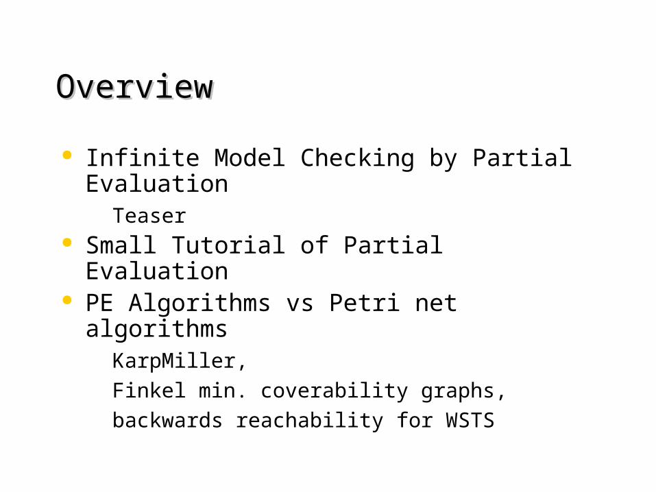
OverviewOverview

Infinite Model Checking by Partial Evaluation– Teaser

Small Tutorial of Partial Evaluation PE Algorithms vs Petri net algorithms

– KarpMiller,

– Finkel min. coverability graphs,

– backwards reachability for WSTS

Part 1:Part 1:

Infinite State Model Checking by Infinite State Model Checking by Partial Evaluation: TeaserPartial Evaluation: Teaser

1. Teaser2. PE Tutorial3. PE vs Petri

(Automatic) Program Optimisation(Automatic) Program Optimisation

When:– Source-to-source

– during compilation

– at link-time

– at run-time Why:

– Make existing programs faster (10 % 500 ...)

– Enable safer, high-level programming style ()

– (Program verification,…)

Program SpecialisationProgram Specialisation

What:– Specialise a program for a

particular application domain How:

– Partial evaluation– Program transformation– Type specialisation– Slicing

DrawingProgram P

P’

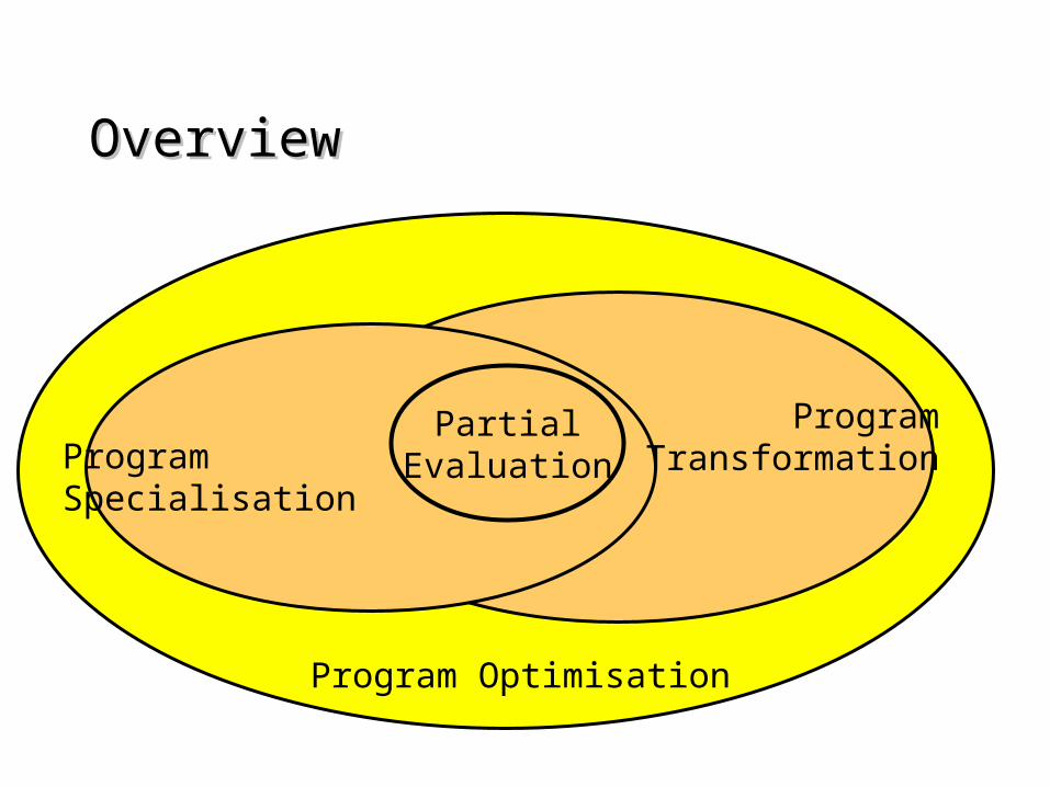
OverviewOverview

PartialEvaluationProgram

Specialisation

ProgramTransformation

Program Optimisation

Ecce Demo IEcce Demo I

=> pUse list notation for goals: [G1,G2].Type a dot (.) and hit return at the end.atom or goal (l for true) =>append([a,b,c,d],L,R).-> calculating static functors-> pre-processing msv phase...-> performing flow analysis.-> removing superfluous polyvariance

-> generating resultants

-> determinate post unfolding.-> dead code removal (DCE).-> redundant argument filtering (RAF). --> 0 arguments erased-> reverse redundant argument filtering (FAR). --> 0 argument(s) erased

/* Specialised program generated by Ecce 1.1 *//* PD Goal: append([a,b,c,d],A,B) *//* Transformation time: 33 ms *//* Unfolding time: 17 ms *//* Post-Processing time: 17 ms */

/* Specialised Predicates: append__1(A,B) :- append([a,b,c,d],A,B). */

append([a,b,c,d],A,[a,b,c,d|A]).append__1(A,[a,b,c,d|A]).

doubleapp(X,Y,Z,XYZ) :- append(X,Y,XY), append(XY,Z,XYZ).

append([],L,L).append([H|X],Y,[H|Z]) :- append(X,Y,Z).

ECCE

Ecce Demo IEcce Demo I

doubleapp(X,Y,Z,XYZ) :- append(X,Y,XY), append(XY,Z,XYZ).

append([],L,L).append([H|X],Y,[H|Z]) :- append(X,Y,Z).

=> pUse list notation for goals: [G1,G2].Type a dot (.) and hit return at the end.atom or goal (l for append([a,b,c,d],_9806,_9807)) =>doubleapp(X,Y,Z,Res).-> calculating static functors-> pre-processing msv phase...-> performing flow analysis..+.++

/* Specialised program generated by Ecce 1.1 *//* PD Goal: doubleapp(A,B,C,D) *//* Transformation time: 83 ms *//* Unfolding time: 0 ms *//* Post-Processing time: 16 ms */

/* Specialised Predicates: doubleapp__1(A,B,C,D) :- doubleapp(A,B,C,D).append_conj__2(A,B,C,D) :- append(A,B,E1), append(E1,C,D).append__3(A,B,C) :- append(A,B,C).*/

doubleapp(A,B,C,D) :- doubleapp__1(A,B,C,D).doubleapp__1([],A,B,C) :- append__3(A,B,C).doubleapp__1([A|B],C,D,[A|E]) :- append_conj__2(B,C,D,E).append_conj__2([],A,B,C) :- append__3(A,B,C).append_conj__2([A|B],C,D,[A|E]) :- append_conj__2(B,C,D,E).append__3([],A,A).append__3([A|B],C,[A|D]) :- append__3(B,C,D).

ECCE

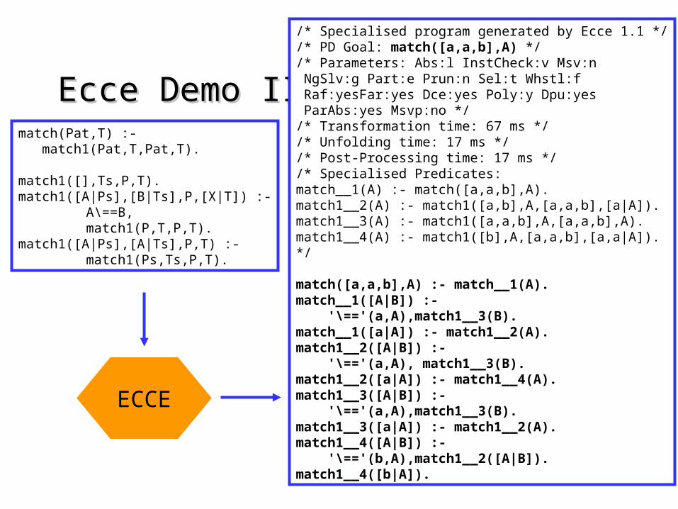
Ecce Demo IIEcce Demo II

/* Specialised program generated by Ecce 1.1 *//* PD Goal: match([a,a,b],A) *//* Parameters: Abs:l InstCheck:v Msv:n NgSlv:g Part:e Prun:n Sel:t Whstl:f Raf:yesFar:yes Dce:yes Poly:y Dpu:yes ParAbs:yes Msvp:no *//* Transformation time: 67 ms *//* Unfolding time: 17 ms *//* Post-Processing time: 17 ms *//* Specialised Predicates: match__1(A) :- match([a,a,b],A).match1__2(A) :- match1([a,b],A,[a,a,b],[a|A]).match1__3(A) :- match1([a,a,b],A,[a,a,b],A).match1__4(A) :- match1([b],A,[a,a,b],[a,a|A]).*/

match([a,a,b],A) :- match__1(A).match__1([A|B]) :- '\=='(a,A),match1__3(B).match__1([a|A]) :- match1__2(A).match1__2([A|B]) :- '\=='(a,A), match1__3(B).match1__2([a|A]) :- match1__4(A).match1__3([A|B]) :- '\=='(a,A),match1__3(B).match1__3([a|A]) :- match1__2(A).match1__4([A|B]) :- '\=='(b,A),match1__2([A|B]).match1__4([b|A]).

match(Pat,T) :- match1(Pat,T,Pat,T).

match1([],Ts,P,T).match1([A|Ps],[B|Ts],P,[X|T]) :-

A\==B,match1(P,T,P,T).

match1([A|Ps],[A|Ts],P,T) :-match1(Ps,Ts,P,T).

ECCE

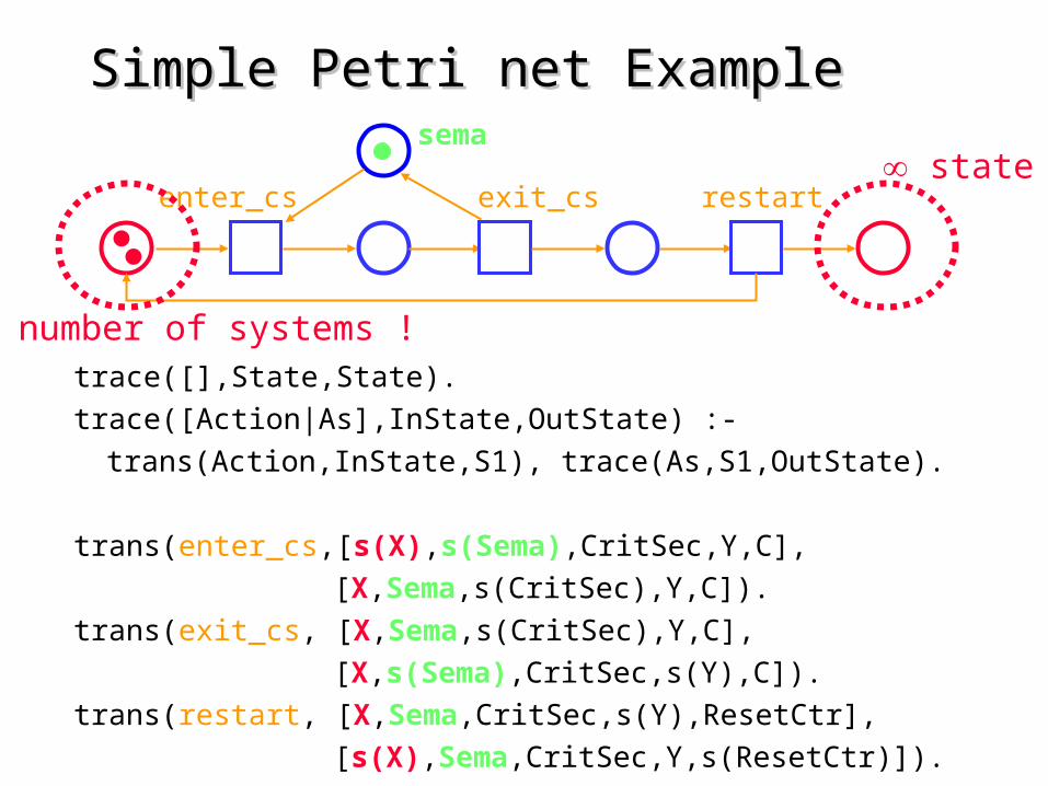
Simple Petri net ExampleSimple Petri net Example

trace([],State,State).

trace([Action|As],InState,OutState) :-

trans(Action,InState,S1), trace(As,S1,OutState).

trans(enter_cs,[s(X),s(Sema),CritSec,Y,C],

[X,Sema,s(CritSec),Y,C]).

trans(exit_cs, [X,Sema,s(CritSec),Y,C],

[X,s(Sema),CritSec,s(Y),C]).

trans(restart, [X,Sema,CritSec,s(Y),ResetCtr],

[s(X),Sema,CritSec,Y,s(ResetCtr)]).

sema

restartexit_csenter_cs state !

number of systems !

Ecce Demo III: Model CheckingEcce Demo III: Model Checkingcs_violation(NumberOfProcesses) :- tr(Tr,NumberOfProcesses,[_,_,s(s(_)),_,_]).

tr(Tr,NumberOfProcesses,State) :- trace(Tr,[NumberOfProcesses,s(0),0,0,0],State).

trace([],State,State).trace([Action|As],InState,OutState) :-

trans(Action,InState,S1),trace(As,S1,OutState).

trans(enter_cs,[s(X),s(Sema),CritSec,Y,C], [X,Sema,s(CritSec),Y,C]).

trans(exit_cs,[X,Sema,s(CritSec),Y,C], [X,s(Sema),CritSec,s(Y),C]).

trans(restart,[X,Sema,CritSec,s(Y),ResetCtr], [s(X),Sema,CritSec,Y,s(ResetCtr)]).

ECCE

/* Specialised program generated by Ecce 1.1 *//* PD Goal: cs_violation(s(0)) *//* Transformation time: 133 ms *//* Unfolding time: 117 ms *//* Post-Processing time: 17 ms */

/* Specialised Predicates: cs_violation__1 :- cs_violation(s(0)).trace__2 :- trace([A1|B1], [s(0),s(0),0,0,s(C1)], [D1,E1,s(s(F1)),G1,H1]).*/

cs_violation(s(0)) :- trace__2.cs_violation__1 :- trace__2.trace__2 :- fail.








ECCE

2 iterations of ECCE (default settings):

cs_violation(s(s(0))) :- cs_violation__1.cs_violation__1 :- trans__2_conj__2.cs_violation__1 :- trace__3__3(0).trans__2_conj__2 :- trans_conj__9__7.trans__2_conj__2 :- trans_conj__5__8(0).trace__3__3(A) :- trans__4_conj__4(A).trace__3__3(A) :- trace__3__3(s(A)).trans__4_conj__4(A) :- trans_conj__5__5(A,B).trans_conj__5__5(A,A) :- trans_conj__5__6(A).trans_conj__5__5(A,s(A)) :- trans_conj__5__5(s(A),s(B)).trans_conj__5__6(A) :- trans_conj__5__5(s(A),s(B)).trans_conj__9__7 :- trans_conj__5__10.trans_conj__9__7 :- trans_conj__5__5(0,A).trans_conj__5__8(A) :- trans_conj__5__9(A).trans_conj__5__8(A) :- trans_conj__5__5(A,B).trans_conj__5__9(A) :- trans_conj__5__5(A,B).trans_conj__5__10 :- trans_conj__5__5(0,A).

After 1 simple bottom-up abstract interpretation:

cs_violation(s(s(0))) :- cs_violation__1.cs_violation__1 :- fail.trans__2_conj__2 :- fail.trace__3__3(A) :- fail.trans__4_conj__4(A) :- fail.trans_conj__5__5(A,A) :- fail.trans_conj__5__5(A,s(A)) :- fail.trans_conj__5__6(A) :- fail.trans_conj__9__7 :- fail.trans_conj__5__8(A) :- fail.trans_conj__5__9(A) :- fail.trans_conj__5__10 :- fail.








ECCE

After 2 Ecce iterations + 1 simple bottom-up abstract interpretation:

cs_violation(s(s(A))) :- cs_violation__1(s(s(A))).cs_violation__1(s(s(A))) :- fail.cs_violation__1(s(A)) :- fail.trans__3_conj__2(A) :- fail.trace__2__3(s(A),B) :- fail.trace__2__3(A,B) :- fail.trans__3_conj__4(A,B) :- fail.trans_conj__4__5(s(A),B) :- fail.trans_conj__4__5(A,B) :- fail.trans_conj__4__6(A,B,B) :- fail.trans_conj__4__6(A,B,s(B)) :- fail.trans_conj__4__7(A,B) :- fail.trans_conj__4__8(s(A),B) :- fail.trans_conj__4__8(A,B) :- fail.trans_conj__4__9(A,B,C,C) :- fail.trans_conj__4__9(A,s(B),C,s(C)) :- fail....trans_conj__4__17(A,s(B),C,s(C)) :- fail.

Ecce Demo: CTL model checkingEcce Demo: CTL model checking/* A Model Checker for CTL fomulas *//* written for XSB-Prolog *//* by Michael Leuschel, Thierry Massart */

sat(_E,true).sat(_E,false) :- fail.sat(E,p(P)) :- prop(E,P). /* proposition */sat(E,and(F,G)) :- sat(E,F), sat(E,G).sat(E,or(F,_G)) :- sat(E,F).sat(E,or(_F,G)) :- sat(E,G).sat(E,not(F)) :- not(sat(E,F)).sat(E,en(F)) :- /* exists next */ trans(_Act,E,E2),sat(E2,F).sat(E,an(F)) :- /* always next */ not(sat(E,en(not(F)))).sat(E,eu(F,G)) :- /* exists until */ sat_eu(E,F,G).sat(E,au(F,G)) :- /* always until */ sat(E,not(eu(not(G),and(not(F),not(G))))), sat_noteg(E,not(G)).sat(E,ef(F)) :- /* exists future */ sat(E,eu(true,F)).sat(E,af(F)) :- /* always future */ sat_noteg(E,not(F)).sat(E,eg(F)) :- /* exists global */ not(sat_noteg(E,F))./* we want gfp -> negate lfp of negation */sat(E,ag(F)) :- /* always global */ sat(E,not(ef(not(F)))).

/* :- table sat_eu/3.*//* tabulation to compute least-fixed point */ sat_eu(E,_F,G) :- /* exists until */ sat(E,G).sat_eu(E,F,G) :- /* exists until */ sat(E,F), trans(_Act,E,E2), sat_eu(E2,F,G).

/* :- table sat_noteg/2.*//* tabulation to compute least-fixed point */

sat_noteg(E,F) :- sat(E,not(F)).sat_noteg(E,F) :- not( (trans(_Act,E,E2), not(sat_noteg(E2,F)))).




prop([X,Sema,s(s(CritSec)),Y,C],unsafe).prop([0,Sema,0,0,C],deadlock).prop([X,0,0,0,C],deadlock).

Infinite Model Checking by P.E.Infinite Model Checking by P.E.

When does it work ?? Why does it work ?? Is it efficient ?? Is it safe ?? How does it compare to existing model checking

algorithms ??

Part 2:Part 2:

Program Optimisation and Partial Program Optimisation and Partial Evaluation: A small tutorialEvaluation: A small tutorial


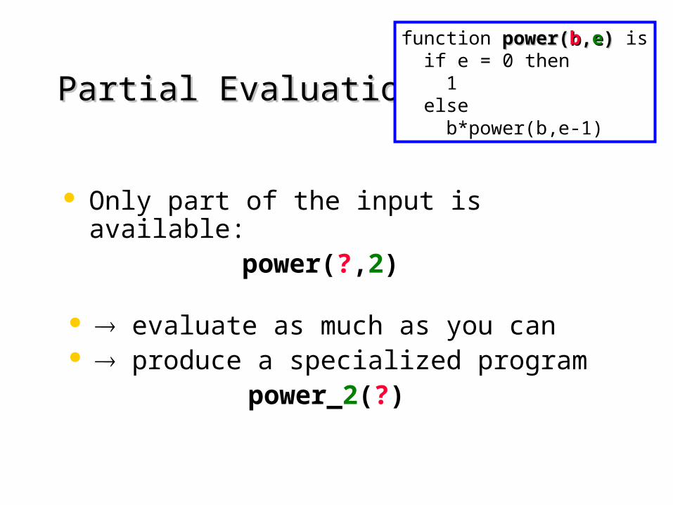
Partial EvaluationPartial Evaluation

Only part of the input is available:power(?,2)

evaluate as much as you can produce a specialized program

power_2(?)

function power(power(bb,,ee)) is if e = 0 then 1 else b*power(b,e-1)

Small ExampleSmall Example

Evaluate + replace call by definition (unfolding)

function power(b,2) is if 2 = 0 then 1 elseelse b*power(b,1)

function power(b,2) is if 2 = 0 then 1 elseelse b* (if 1 = 0 then 1 elseelse b*power(b,0))

function power(b,2) is if 2 = 0 then 1 elseelse b* (if 1 = 0 then 1 elseelse b* (if 0 = 0 then 1then 1 else b*power(b,-1)))

function power_2(b) is b*b*1

Residual code:

≈ SQR function

function power(power(bb,,ee)) is if e = 0 then 1 else b*power(b,e-1)

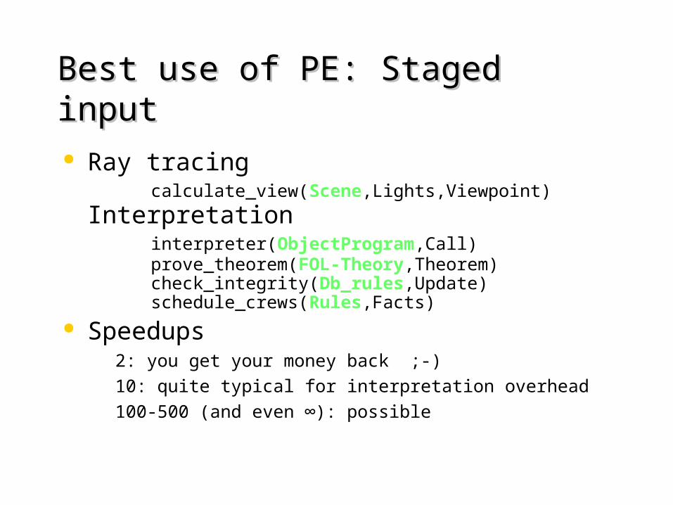
Best use of PE: Staged inputBest use of PE: Staged input

Ray tracingcalculate_view(Scene,Lights,Viewpoint)

Interpretationinterpreter(ObjectProgram,Call)prove_theorem(FOL-Theory,Theorem)check_integrity(Db_rules,Update)schedule_crews(Rules,Facts)

Speedups– 2: you get your money back ;-)– 10: quite typical for interpretation overhead– 100-500 (and even ∞): possible

Ray TracingRay Tracing

Static

Partial Evaluation for Logic Partial Evaluation for Logic Programming (Partial Deduction)Programming (Partial Deduction)

Principles and CorrectnessPrinciples and Correctness

Logical Foundation: SLD-ResolutionLogical Foundation: SLD-Resolution

Selection-rule driven Linear Resolution for Definite Clauses

Selection-rule– In a denial: selects a literal to be resolved

Linear Resolution– Derive new denial, forget old denial

Definite Clauses:– Limited to (Definite) Program Clauses

– (Normal clause: negation allowed in body)

knows_logic(X) good_student(X) teacher(Y,X) logician(Y)

good_student(tom) good_student(jane) logician(peter) teacher(peter,tom)

SLD-TreesSLD-Trees knows_logic(Z)

good_student(X) teacher(Y,X) logician(Y)

teacher(Y,tom) logician(Y)

logician(peter)

teacher(Y,jane) logician(Y)

Prolog: explores this tree Depth-First, always selects leftmost literal

fail

What is Full Evaluation in LPWhat is Full Evaluation in LP

In our context: full evaluation =constructing complete SLD-tree for a goal every branch either

successful, failed or infinite

SLD can handle variables !! can handle partial data-structures

(not the case for imperative or functional programming)

Unfolding = ordinary SLD-resolution !

Partial evaluation = full evaluation ??

Partial evaluation trivial ??

ExampleExampleapp([],L,L).app([H|X],Y,[H|Z]) :- app(X,Y,Z).

app ([a],B,C)

app ([],B,C’)

{C/[a|C’]}

{C’/B}

app([a],B,[a|B]).

app_a(B,[a|B]).

Apply c.a.s. oninitial goal

(+ filter out static part)

Example IIExample II

BUT: complete SLD-tree usually infinite !!

app([],L,L).app([H|X],Y,[H|Z]) :- app(X,Y,Z).

app (A,[a],B)

app (A’,[a],B’)

{A/[],B/[a]} {A/[H|A’],B/[H|B’]}

app (A’’,[a],B’’)

{A’/[],B’/[a]} {A’/[H|A’’],B’/[H|B’’]}

...

Partial DeductionPartial Deduction

Basic Principle:– Instead of building one complete SLD-tree:

Build a finite number of finite “SLD- trees” !

– SLD-trees can be incomplete 4 types of derivations in SLD-trees:

– Successful, failed, infinite

– Incomplete: no literal selected

Main issues in PD (& PE in general)Main issues in PD (& PE in general)

How to construct the specialised code ? When to stop unfolding (building SLD-tree) ? Construct SLD-trees for which goals ? When is the result correct ?

Generating Code:Generating Code:ResultantsResultants Resultant of

SLD-derivation

is the formula: G01...k Gk

if n=1: Horn clause !

A1,…,Ai,…,An

G1

G2

...

Gk

0

1

k

G0

Resultants: ExampleResultants: Example

app([],L,L).app([H|X],Y,[H|Z]) :- app(X,Y,Z).

app (A,[a],B)

app (A’,[a],B’)

{A/[],B/[a]} {A/[H|A’],B/[H|B’]}

app([],[a],[a]).app([H|A’],[a],[H|B’]) :- app(A’,[a],B’).

STOP

Formalisation of Partial DeductionFormalisation of Partial Deduction

Given a set S = {A1,…,An} of atoms: Build finite, incomplete SLD-trees for each Ai

For every non-failing branch:– generate 1 specialised clause by

computing the resultants

When is this correct ?

Correctness 1: Non-trivial treesCorrectness 1: Non-trivial treesCorrectness 2: ClosednessCorrectness 2: Closednessapp([],L,L).app([H|X],Y,[H|Z]) :- app(X,Y,Z).

app ([a|A],B,C)

app (A,B,C’)

{C/[a|C’]}

app([a|A],B,[a|C’]) :- app(A,B,C’).

Stop

app ([a,b],[],C)

app ([b],[],C)

fail

Not: C/[a,b] !!Not an instance ofapp ([a|A],B,C)

Closedness ConditionClosedness Condition

To avoid uncovered calls at runtime:

All predicate calls– - in the bodies of specialised clauses

(= atoms in leaves of SLD-trees !)

– - and in the calls to the specialised program must be instances of at least one of the atoms in

S = {A1,…,An}

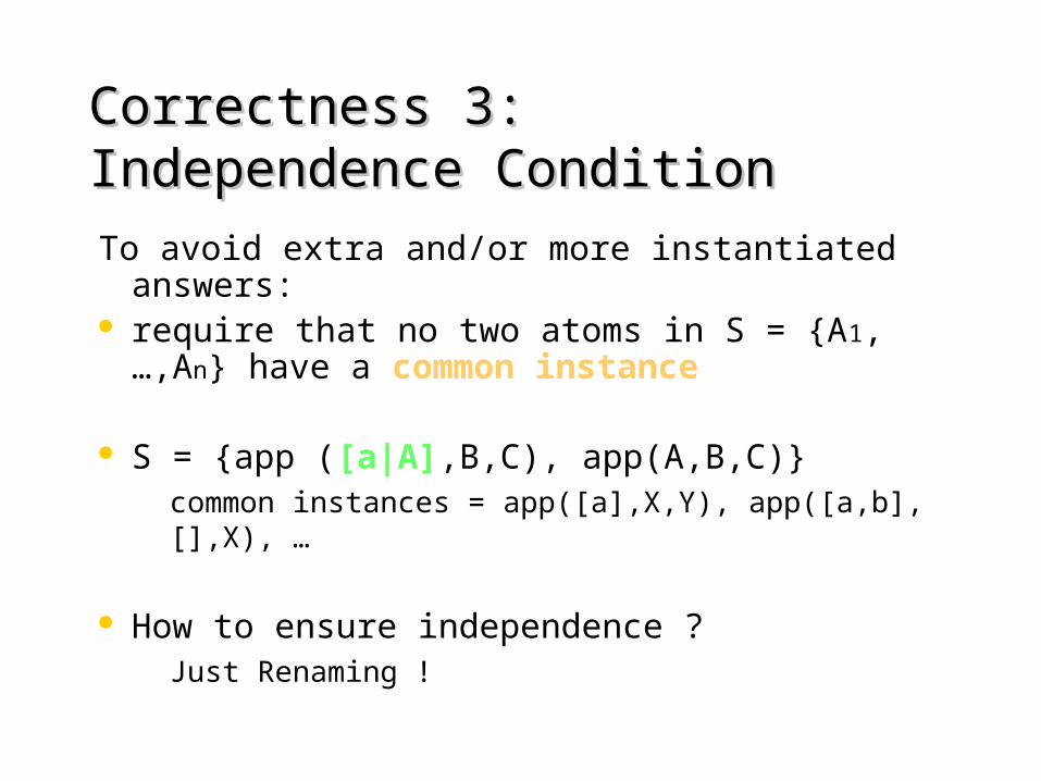
Correctness 3:Correctness 3:Independence ConditionIndependence Condition

To avoid extra and/or more instantiated answers: require that no two atoms in S = {A1,…,An} have

a common instance

S = {app ([a|A],B,C), app(A,B,C)}– common instances = app([a],X,Y), app([a,b],[],X), …

How to ensure independence ?– Just Renaming !

Soundness & CompletenessSoundness & Completeness

P’ obtained by partial deduction from P

If non-triviality, closedness, independence conditions are satisfied:

P’ {G} has an SLD-refutation with c.a.s. iff P {G}has

P’ {G} has a finitely failed SLD-tree iffP {G}has

Lloyd, Shepherdson: J. Logic Progr. 1991

A more detailed exampleA more detailed example

map (inv,L,R)

{L/[],R/[]}

C=..[inv,H,PH], call(C),map(inv,L’,R’)

{L/[H|L’],R/[PH|R’]}

inv(H,PH),map(inv,L’,R’)

call(inv(H,PH)),map(inv,L’,R’)

{C/inv(H,PH)}map(inv,[],[]).map(inv,[0|L’],[1|R’]) :- map(inv,L’,R’).map(inv,[1|L’],[0|R’]) :- map(inv,L’,R’).

map(inv,L’,R’)

{H/0,PH/1}

map(inv,L’,R’)

{H/1,PH/0}

map(P,[],[]).map(P,[H|T],[PH|PT]) :- C=..[P,H,PH], call(C),map(P,T,PT).inv(0,1).inv(1,0).

Overhead removed: 2 faster

map_1([],[]).map_1([0|L’],[1|R’]) :- map_1(L’,R’).map_1([1|L’],[0|R’]) :- map_1(L’,R’).

Controlling Partial Deduction:Controlling Partial Deduction:Local vs global controlLocal vs global control

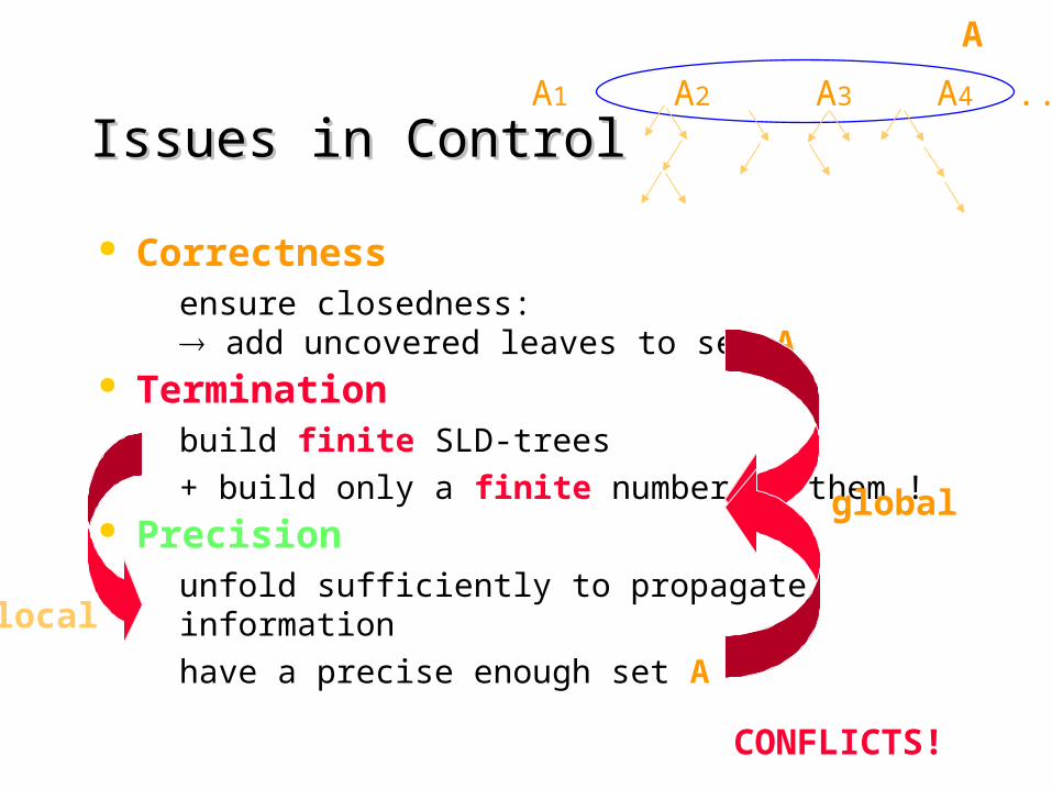
Issues in ControlIssues in Control

Correctness– ensure closedness:

add uncovered leaves to set A Termination

– build finite SLD-trees

– + build only a finite number of them ! Precision

– unfold sufficiently to propagate information

– have a precise enough set A

global

local

A1 A2 A3 A4 ...

A

CONFLICTS!

Control:Control:Local vs GlobalLocal vs Global Local Control:

– Decide upon the individual SLD-trees– Influences the code generated for each Ai

unfolding rule given a program P and goal G returns finite, possibly

incomplete SLD-tree

Global control– decide which atoms are in A

abstraction operator

A1 A2 A3 A4 ...

A

Generic AlgorithmGeneric Algorithm

Input: program P and goal GOutput: specialised program P’Initialise: i=0, A0 = atoms in G

repeat Ai+1 := Ai

for each a Ai do Ai+1 := Ai+1 leaves(unfold(a)) end for Ai+1 := abstract(Ai+1) until Ai+1 = Ai

compute P’ via resultants+renaming

Controlling Partial Deduction:Controlling Partial Deduction:LocalLocal Control & Control & TerminationTermination

Local Termination:Local Termination:Well-founded ordersWell-founded orders < (strict) partial order (transitive, anti-reflexive,

anti-symmetric) with no descending chainss1 > s2 > s3 >…

To ensure termination:– define < on expressions/goals

– unfold only if sk+1 < sk

Example: termsize norm (number of function and constant symbols)

Mapping to

ExampleExampleapp([],L,L).app([H|X],Y,[H|Z]) :- app(X,Y,Z).

app ([a,b|C],A,B)

app ([b|C],A,B’)

{B/[a|A’]}

Unificationfails

app (C,A,B’’)

{B’/[b|A’’]}

Unificationfails Stop

app (C’,A,B’’’)

{C/[H|C’],B’’/[H|A’’’]}

|.| = 3

|.| = 5

|.| = 1

|.| = 1|.| = 0

Ok

Ok

Local termination:Local termination:Well-quasi ordersWell-quasi orders quasi order (reflexive and transitive) with

every infinite sequence s1,s2,s3,… we can findi<j such that si sj

To ensure termination:– define on expressions/goals

– unfold only if for no i<k+1: si sk+1

Comparison: WFO’s and WQO’sComparison: WFO’s and WQO’s

No descending chains s1 > s2 > s3 >…

Ensure that sk+1 < sk

More efficient(only previous element)

Can be used statically– (admissible sequences can

be composed)

Every sequence:si sj with i<j

Ensure that not si sk+1

– uncomparable elements

More powerful (L.SAS’98)

more powerful than all monotonic and simplification orderings

Homeomorphic Embedding Homeomorphic Embedding

Diving: s f(t1,…,tn) if i: s ti

Coupling: f(s1,…,sn) f(t1,…,tn) if i: si ti

n≥0

f(a) g(f(f(a)),a)

f

a

g

a

f

f

a

Admissible transitionsAdmissible transitions

rev([a,b|T],[],R)

solve(rev([a,b|T],[],R),0)

t(solve(rev([a,b|T],[],R),0),[])

path(a,b,[])

path(b,a,[])

t(solve(path(a,b,[]),0),[])

rev([a|T],[a],R)

solve(rev([a|T],[a],R),s(0))

t(solve(rev([a|T],[a],R),s(0)),[rev]))

path(b,a,[a])

path(a,b,[b])

t(solve(path(b,a,[a]),s(0)),[path]))

Higman-Kruskal Theorem (1952/60)Higman-Kruskal Theorem (1952/60)

is a WQO (over a finite alphabet) Infinite alphabets + associative operators:

f(s1,…,sn) g(t1,…,tm) if f g andi: si tji

with 1j1<j2<…<jnm

and(q,p(b)) and(r,q,p(f(b)),s)

Variables : X Y more refined solutions possible (DSSE-TR-98-11)

Controlling Partial Deduction:Controlling Partial Deduction:GlobalGlobal control and control and abstractionabstraction

Most Specific Generalisation (msg)Most Specific Generalisation (msg)

A is more general than B iff : B=A

for every B,C there exists a most specific generalisation (msg) M:– M more general than B and C

– if A more general then B and C then A is also more general than M

there exists an algorithm for computing the msg

(anti-unification, least general generalisation)

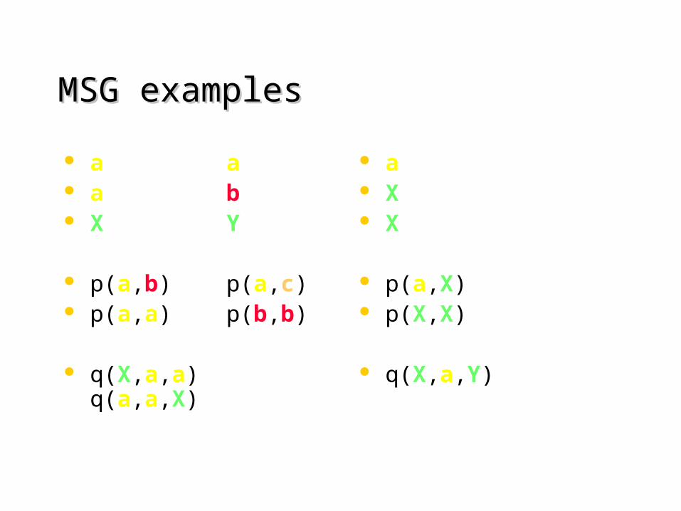
MSG examplesMSG examples

a a a b X Y

p(a,b) p(a,c) p(a,a) p(b,b)

q(X,a,a) q(a,a,X)

a X X

p(a,X) p(X,X)

q(X,a,Y)

First abstraction operatorFirst abstraction operator

[Benkerimi,Lloyd’90] abstract two atoms in Ai+1 by their msg if they have a common instance

will also ensureindependence(no renaming required)

Termination ?

Input: program P and goal GOutput: specialised program P’Initialise: i=0, A0 = atoms in G

repeat Ai+1 := Ai

for each a Ai do Ai+1 := Ai+1 leaves(unfold(a)) end for Ai+1 := abstract(Ai+1) until Ai+1 = Ai

compute P’ via resultants+renaming

Rev-accRev-accrev([],L,L).rev([H|X],A,R) :- rev(X,[H|A],R).

rev (L,[],R)

rev (L’,[H],R)

rev (L’’,[H’,H],R)

rev (L’,[H],R)

rev (L’’’,[H’’,H’,H],R)

rev (L’’,[H’,H],R)

unfold

unfold

unfold

rev(L,[],R)

rev(L’,[H],R)rev(L’’,[H’,H],R)

rev(L’’’,[H’’,H’,H],R)

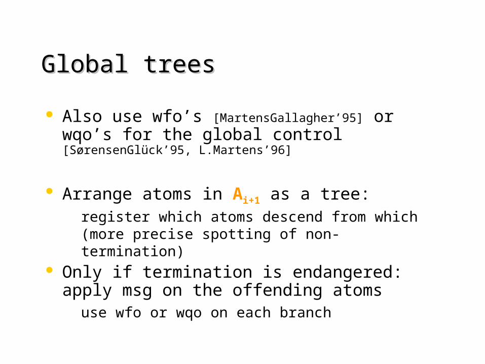
Global treesGlobal trees

Also use wfo’s [MartensGallagher’95] or wqo’s for the global control [SørensenGlück’95, L.Martens’96]

Arrange atoms in Ai+1 as a tree:– register which atoms descend from which

(more precise spotting of non-termination) Only if termination is endangered: apply msg on

the offending atoms– use wfo or wqo on each branch

Other improvementsOther improvements

Characteristic trees (L. et al: Toplas’98)

Conjunctive partial deduction (JLP’99)

Integrate with abstract interpretation– In classical PD: a call stands for all its instances

– Allow more refined domains (regular types,…)

Part 3:Part 3:

Online Partial Evaluation and Petri Online Partial Evaluation and Petri net algorithmsnet algorithms


online partial evaluation, infinite model checking, and petri net algorithms

Documents