University of Tennessee, Knoxville University of Tennessee, Knoxville

TRACE: Tennessee Research and Creative TRACE: Tennessee Research and Creative

Exchange Exchange

Masters Theses Graduate School

12-2018

Online Machine Learning Algorithms Review and Comparison in Online Machine Learning Algorithms Review and Comparison in

Healthcare Healthcare

Nikhil Mukund Jagirdar University of Tennessee, njagirda@vols.utk.edu

Follow this and additional works at: https://trace.tennessee.edu/utk_gradthes

Recommended Citation Recommended Citation Jagirdar, Nikhil Mukund, "Online Machine Learning Algorithms Review and Comparison in Healthcare. " Master's Thesis, University of Tennessee, 2018. https://trace.tennessee.edu/utk_gradthes/5393

This Thesis is brought to you for free and open access by the Graduate School at TRACE: Tennessee Research and Creative Exchange. It has been accepted for inclusion in Masters Theses by an authorized administrator of TRACE: Tennessee Research and Creative Exchange. For more information, please contact trace@utk.edu.

To the Graduate Council:

I am submitting herewith a thesis written by Nikhil Mukund Jagirdar entitled "Online Machine

Learning Algorithms Review and Comparison in Healthcare." I have examined the final electronic

copy of this thesis for form and content and recommend that it be accepted in partial fulfillment

of the requirements for the degree of Master of Science, with a major in Industrial Engineering.

Xueping Li, Major Professor

We have read this thesis and recommend its acceptance:

Jamie Coble, John Kobza

Accepted for the Council:

Dixie L. Thompson

Vice Provost and Dean of the Graduate School

(Original signatures are on file with official student records.)

Online Machine Learning Algorithms

Review and Comparison in Healthcare

A Thesis Presented for the

Master of Science

Degree

The University of Tennessee, Knoxville

Nikhil Mukund Jagirdar

December 2018

c© by Nikhil Mukund Jagirdar, 2018

All Rights Reserved.

ii

dedication...

iii

Acknowledgments

I am indebted to my thesis advisor, Dr. Xueping Li of the Department of Industrial and

Systems Engineering at the University of Tennessee-Knoxville. I will be eternally grateful

for his patience, inspiration, and kindness as a mentor and a friend.

I am also extremely grateful to the thesis committee members, Dr. John E. Kobza, and

Dr. Jamie Baalis Coble, for reviewing my work regularly and providing me with valuable

feedback.

Finally, I thank my parents, Mukund and Vandana, my brothers, Rohan and Ninad,

and my friends, Prafulla, Amol, Abhishek, Ray, Nitin, and Suyash, for supporting and

encouraging me.

iv

Abstract

Currently, the healthcare industry uses Big Data for essential patient care information.

Electronic Health Records (EHR) store massive data and are continuously updated with

information such as laboratory results, medication, and clinical events. There are various

methods by which healthcare data is generated and collected, including databases, healthcare

websites, mobile applications, wearable technologies, and sensors. The continuous flow of

data will improve healthcare service, medical diagnostic research and, ultimately, patient

care. Thus, it is important to implement advanced data analysis techniques to obtain more

precise prediction results.

Machine Learning (ML) has acquired an important place in Big Healthcare Data (BHD).

ML has the capability to run predictive analysis, detect patterns or red flags, and connect

dots to enhance personalized treatment plans. Because predictive models have dependent

and independent variables, ML algorithms perform mathematical calculations to find the

best suitable mathematical equations to predict dependent variables using a given set of

independent variables. These model performances depend on datasets and response, or

dependent, variable types such as binary or multi-class, supervised or unsupervised.

The current research analyzed incremental, or streaming or online, algorithm performance

with offline or batch learning (these terms are used interchangeably) using performance

measures such as accuracy, model complexity, and time consumption. Batch learning

algorithms are provided with the specific dataset, which always constrains the size of the

dataset depending on memory consumption. In the case of incremental algorithms, data

arrive sequentially, which is determined by hyperparameter optimization such as chunk size,

tree split, or hoeffding bond. The model complexity of an incremental learning algorithm is

based on a number of parameters, which in turn determine memory consumption.

v

Table of Contents

1 Introduction 1

1.1 Big Data in Healthcare . . . . . . . . . . . . . . . . . . . . . . . . . . . . . . 1

1.2 Predictive analytics in Big Healthcare Data / Big Data Analytics . . . . . . 3

1.2.1 Predictive modeling process . . . . . . . . . . . . . . . . . . . . . . . 3

1.2.2 Predictive analysis using batch learning . . . . . . . . . . . . . . . . . 4

1.2.3 Predictive analysis using incremental learning . . . . . . . . . . . . . 5

1.3 Challenges in batch learning . . . . . . . . . . . . . . . . . . . . . . . . . . . 5

1.4 Challenges in incremental learning . . . . . . . . . . . . . . . . . . . . . . . . 6

1.4.1 Concept drift and data distribution change . . . . . . . . . . . . . . . 6

1.4.2 Catastrophic Forgetting . . . . . . . . . . . . . . . . . . . . . . . . . 7

1.4.3 Model Complexity . . . . . . . . . . . . . . . . . . . . . . . . . . . . 7

1.4.4 Performance Evaluation and model benchmarking . . . . . . . . . . . 7

2 Literature Review 8

2.1 Machine learning in healthcare . . . . . . . . . . . . . . . . . . . . . . . . . . 9

2.2 Online machine learning applications . . . . . . . . . . . . . . . . . . . . . . 10

2.3 Offline Machine learning Methods . . . . . . . . . . . . . . . . . . . . . . . . 10

2.3.1 Linear Regression . . . . . . . . . . . . . . . . . . . . . . . . . . . . . 10

2.3.2 Support Vector Machine (SVM) . . . . . . . . . . . . . . . . . . . . . 11

2.4 Online Machine learning Algorithm . . . . . . . . . . . . . . . . . . . . . . . 12

2.5 Concept Drift . . . . . . . . . . . . . . . . . . . . . . . . . . . . . . . . . . . 13

2.6 Competitive Ratio . . . . . . . . . . . . . . . . . . . . . . . . . . . . . . . . 13

vi

3 Algorithm 15

3.1 Offline or batch learning algorithm . . . . . . . . . . . . . . . . . . . . . . . 15

3.1.1 Naive Bayes : NB . . . . . . . . . . . . . . . . . . . . . . . . . . . . . 16

3.1.2 Logistic Regression: LR . . . . . . . . . . . . . . . . . . . . . . . . . 16

3.1.3 Back-propagation Neural Network : NN . . . . . . . . . . . . . . . . 17

3.1.4 Random Forest . . . . . . . . . . . . . . . . . . . . . . . . . . . . . . 18

3.1.5 Adaptive Boosting (AdaBoost) . . . . . . . . . . . . . . . . . . . . . 19

3.2 Online or Incremental Learning Algorithm . . . . . . . . . . . . . . . . . . . 20

3.2.1 Learn++ . . . . . . . . . . . . . . . . . . . . . . . . . . . . . . . . . 20

3.2.2 Incremental Random Forest . . . . . . . . . . . . . . . . . . . . . . . 22

3.2.3 Hoeffding Tree . . . . . . . . . . . . . . . . . . . . . . . . . . . . . . 22

4 Experiment 26

4.1 Datasets . . . . . . . . . . . . . . . . . . . . . . . . . . . . . . . . . . . . . . 26

4.1.1 Mortality Data . . . . . . . . . . . . . . . . . . . . . . . . . . . . . . 26

4.1.2 Diabetic burnout Data . . . . . . . . . . . . . . . . . . . . . . . . . . 27

4.2 Data preparation & Model Evaluation . . . . . . . . . . . . . . . . . . . . . 27

4.2.1 Performance Evaluation . . . . . . . . . . . . . . . . . . . . . . . . . 28

4.2.2 Cross Validation . . . . . . . . . . . . . . . . . . . . . . . . . . . . . 29

4.2.3 Bootstrap and Bagging . . . . . . . . . . . . . . . . . . . . . . . . . . 30

4.3 Hyper-parameters and Model Complexity . . . . . . . . . . . . . . . . . . . . 30

4.4 Results . . . . . . . . . . . . . . . . . . . . . . . . . . . . . . . . . . . . . . . 31

4.4.1 Batch/off-line learning results . . . . . . . . . . . . . . . . . . . . . . 31

4.4.2 Incremental/on-line learning results . . . . . . . . . . . . . . . . . . . 37

5 Conclusions and Future Research 39

Bibliography 41

Appendices 46

A Summary of Equations . . . . . . . . . . . . . . . . . . . . . . . . . . . . . . 47

B Summary of Code . . . . . . . . . . . . . . . . . . . . . . . . . . . . . . . . . 50

vii

C Summary of Confusion Matrix . . . . . . . . . . . . . . . . . . . . . . . . . . 50

C.1 Offline machine learning . . . . . . . . . . . . . . . . . . . . . . . . . 50

C.2 Online machine learning . . . . . . . . . . . . . . . . . . . . . . . . . 51

Vita 52

viii

List of Tables

4.1 The evaluated Datasets and their characteristics . . . . . . . . . . . . . . . . 26

4.2 Mortality Data . . . . . . . . . . . . . . . . . . . . . . . . . . . . . . . . . . 27

4.3 Diabetic burnout Data . . . . . . . . . . . . . . . . . . . . . . . . . . . . . . 28

4.4 Model accuracy comparison . . . . . . . . . . . . . . . . . . . . . . . . . . . 31

C.1 Naive Bayes’ algorithm confusion matrix . . . . . . . . . . . . . . . . . . . . 50

C.2 Mortality Data NB . . . . . . . . . . . . . . . . . . . . . . . . . . . . . . . . 50

C.3 Diabetic Data NB . . . . . . . . . . . . . . . . . . . . . . . . . . . . . . . . . 50

C.4 Logistic regression algorithm confusion matrix . . . . . . . . . . . . . . . . . 50

C.5 Mortality Data LR . . . . . . . . . . . . . . . . . . . . . . . . . . . . . . . . 50

C.6 Diabetic Data LR . . . . . . . . . . . . . . . . . . . . . . . . . . . . . . . . . 50

C.7 Random forest algorithm confusion matrix . . . . . . . . . . . . . . . . . . . 50

C.8 Mortality Data RF . . . . . . . . . . . . . . . . . . . . . . . . . . . . . . . . 50

C.9 Diabetic Data RF . . . . . . . . . . . . . . . . . . . . . . . . . . . . . . . . . 50

C.10 AdaBoost algorithm confusion matrix . . . . . . . . . . . . . . . . . . . . . . 51

C.11 Mortality Data AdaBoost . . . . . . . . . . . . . . . . . . . . . . . . . . . . 51

C.12 Diabetic Data AdaBoost . . . . . . . . . . . . . . . . . . . . . . . . . . . . . 51

C.13 Learn++ algorithm confusion matrix . . . . . . . . . . . . . . . . . . . . . . 51

C.14 Mortality Data Learn++ . . . . . . . . . . . . . . . . . . . . . . . . . . . . . 51

C.15 Diabetic Data Learn++ . . . . . . . . . . . . . . . . . . . . . . . . . . . . . 51

C.16 Incremental random forest algorithm confusion matrix . . . . . . . . . . . . 51

C.17 Mortality Data IRF . . . . . . . . . . . . . . . . . . . . . . . . . . . . . . . . 51

C.18 Diabetic Data IRF . . . . . . . . . . . . . . . . . . . . . . . . . . . . . . . . 51

ix

C.19 Hoeffding tree algorithm confusion matrix on Diabetic data . . . . . . . . . . 51

x

List of Figures

1.1 Exponential growth in data [8]. . . . . . . . . . . . . . . . . . . . . . . . . . 2

1.2 Big Data Predictive analytic process. . . . . . . . . . . . . . . . . . . . . . . 4

1.3 A representation of the batch machine learning scheme . . . . . . . . . . . . 5

1.4 The online learning scheme [22]. . . . . . . . . . . . . . . . . . . . . . . . . . 6

2.1 SVM algorithm representation . . . . . . . . . . . . . . . . . . . . . . . . . . 12

3.1 A representation of Neural Network classifier. . . . . . . . . . . . . . . . . . 18

3.2 Learn++ algorithm from [22] . . . . . . . . . . . . . . . . . . . . . . . . . . 21

3.3 Incremental random forest flow diagram . . . . . . . . . . . . . . . . . . . . 23

3.4 Hoeffding Tree algorithm from [9] . . . . . . . . . . . . . . . . . . . . . . . . 24

3.5 Data stream classification cycle in MOA . . . . . . . . . . . . . . . . . . . . 25

4.1 Cross Validation . . . . . . . . . . . . . . . . . . . . . . . . . . . . . . . . . . 29

4.2 Cross-validation results of offline learning accuracy vs fold mortality dataset. 32

4.3 Cross-validation results of offline learning accuracy vs fold on diabetic dataset. 33

4.4 Random forest variable importance for Mortality dataset. . . . . . . . . . . . 35

4.5 Random forest variable importance for Mortality dataset. . . . . . . . . . . . 36

4.6 Learn++ algorithm error graph . . . . . . . . . . . . . . . . . . . . . . . . . 38

xi

Chapter 1

Introduction

The healthcare industry records large datasets which are essential for patient care,

determining preventive diagnostic methods, compliance, and regulatory requirements.

Electronic health records (EHRs) store massive data digitally through various software such

as Pediatric Therapy EMR, NextGen Healthcare, and athenaClinicals. EHRs contain patient

information that may include demographics, medical history, laboratory results, medication,

clinical events, personal statistics like age and weight, and billing information. The Internet

of Things (IoT) has increased the growth and scope of healthcare data with features such as

internet-enabled blood pressure monitors, mHealth apps, and wearable technologies.

1.1 Big Data in Healthcare

Big Healthcare Data (BHD) refers to complex datasets that have some unique characteristics,

beyond their large size, that both facilitate and convolute the process of extraction of

actionable knowledge about an observable phenomenon. According to a recent study

published by Market Research Future, the global market of Big Data in healthcare is forecast

to reach approximately $35 billion by 2021, at a striking rate of CAGR ; during the forecast

period 2016−2021. There is has been an exponential increase observed in the Big Data

size and complexity; however, the lifespan of the data rapidly decays at an exponential rate

(Figure 1.1).

1

Figure 1.1: Exponential growth in data [8].

Increasing BHD faced with various challenges such as resource cost, precision of diagnostic

or preventive prediction to improve patient care, and use of data considering rapid decrease

of its lifespan. As healthcare organizations are moving towards real-time data analytics

with the aim to gain actionable insights and personalized services, challenges remain how to

harness the ever growing data generated continuously.

Model-based techniques have a fixed number of parameters and postulate explicitly their

probability distributions, whereas non-parametric methods relax the a priori beliefs of the

parameter distributions and allow varying number of parameters, relative to the amount of

training data [8].

BHD is often unstructured data which can be produced through EHR, wearable device,

social media. An initial analysis may involve taking care of missing data, identifying

redundant information, classifying data for desired prediction. Another challenge of sharing

EHR data is a concern with patient privacy, has to be a high priority in order to comply

with the EU Directive 95/46/CE and the HIPAA privacy rule [14].

While researchers are still debating the definitions and boundaries of Big Data in health,

benefits of health-related Big Data have been demonstrated in three areas so far, namely to

2

1) prevent disease, 2) identify modifiable risk factors for disease, and 3) design interventions

for health behavior change [14].

1.2 Predictive analytics in Big Healthcare Data / Big

Data Analytics

Various machine learning algorithms are used in Big Healthcare Data analytics for making

decisions using predictive analysis (Figure 1.2). Google has recently developed machine

learning algorithm to help detect cancer with 98% accuracy.

In an incremental predictive analysis, BHD can be used as a hypothesis for the new data

rather than as a firm prediction. Recently, incremental or online machine learning algorithms

have played a growing role in various big data applications such as healthcare, e-commerce,

and social media; the healthcare industry in particular accesses a tremendous amount data

recorded electronically and with cloud-computing services. With increasing compliance and

regulatory requirements and a mounting patient care load, this massive data must be used

to obtain more accurate diagnostic predictions.

The current discussion analyzes different offline and online classification and regression

techniques. Modern-day predictive analytic techniques are useful in forecasting trends

using retrospective and current data by recognizing adverse events or deteriorating patient

conditions or behaviors before the actual events and identifying unusual patterns in the data.

Traditional offline, or batch learning, is limited in memory size, time, and cost.

1.2.1 Predictive modeling process

In data mining given data, Di = (xi, yi) is divided first for predictive modeling into three

sets:

• Training set - In which observations are used to train the model with one or more

algorithm.

• Validation set - In which validation data is used to predict the model and find best

model. This process is also known as tuning.

3

Figure 1.2: Big Data Predictive analytic process.

• Testing set - This set is used to predict final model performance.

There are various techniques to split the data such as even/odd, venetian blinds, random,

and visual inspection. In this paper, data analyzed is healthcare data so random split

technique is utilized to define train, validation, and test datasets.

1.2.2 Predictive analysis using batch learning

A batch algorithm develops a decision model on the entire sequence at once (Figure 1.3). The

predictive model (aka machine learning) is a statistical process that forecasts the outcome

of a particular event occurrence which is response or dependent variable using independent

or predictor variables from the dataset. In machine learning, classification of the model

can be either supervised or unsupervised. Supervised learning can evaluate observations

using training set predictor variables; unsupervised learning uses clustering as classification

procedure. The current study analyzed supervised healthcare data. For instance, a response

variable yi ∈ 1,..,c given as set of features Xi = (xi,1, xi,2,...,xi,p) ∈ Rp. The response variable

can be multi-class or binary {0,1}.

4

Figure 1.3: A representation of the batch machine learning scheme

1.2.3 Predictive analysis using incremental learning

Large dataset batch learning is not cost effective; also, in most cases one day’s data sequence

arrives over time (Figure 1.4). In order to keep the model updated with changes in data

and features, incremental machine learning applications are used. For instance, in sequential

supervised data: arrive {(xi,yi)} ti=1 and t be set of sequences. Each sequence contains (xi,yi)

where xi = 〈 xi,1, xi,2, ...,xi,N 〉 and yi = 〈 yi,1, yi,2, ...,yi,N 〉. The goal is to construct the

classifier h to predict label yt for given x. The loss function L(y, y) is determined for each

model. Then prediction of final t model can be formulated as yt = ht−1(xt).

The online accuracy of model at time t is given by [22]:

E(S) =1

t

t∑i=1

1− L(hi−1(xi), yi) (1.1)

1.3 Challenges in batch learning

The batch learning algorithm has limitations when it comes to non-stationary datasets. The

data flow is continuous in healthcare applications; however, batch learning algorithms can

not offer dynamic adaption of the model based on when new data arrives [30]. Streaming

of the new data may have time-varying domain, and it may vary in terms of probabilistic

5

Figure 1.4: The online learning scheme [22].

distribution of the arrival data. This makes batch learning even more complex and requires

more computation resources. Batch learning has inconsistency over the data. Subsequent

models in batch learning are unrelated [6]. The high volume of data takes time and memory

with batch learning and may also lead to an outdated model.

1.4 Challenges in incremental learning

1.4.1 Concept drift and data distribution change

Incremental algorithms with large data can result in time inefficiency, for instance

distribution frequency sometime has error bound. Such a problem can be solved using

sampling. This process stream error is within the space of computational resources in data

stream system management error margins. There is always a trade-off between accuracy and

amount of memory [28]. However, certain batch learning models, such as C4.5, work in linear

time, whereas incremental models increase computation efforts. The incremental cost can be

more than the overall batch learning computational cost [6]. Changes in data distribution

over time are referred to as concept drift. As a learner is unable to predict arriving data

distribution, concept drift is unpredictable [19]. The section 2.5 explains SMOTE (Synthetic

Minority Oversampling Technique) algorithm employed to overcome concept drift challenge

in the incremental model.

6

1.4.2 Catastrophic Forgetting

As new data arrives, incremental algorithms create a new decision model and forget the old

in order to meet memory and time constraints,. In some situations, maintaining a decision

model may be preferable. This behavior of incremental learning is known as catastrophic

forgetting [26]. As discussed above, there are always trade-off dilemmas when working with

accurate prediction and computational resource limitations for artificial or biological learning

systems, which is known as a stability-plasticity dilemma. One way to deal with this problem

is a just-in-time (JIT) classifier or online/offline hybrid algorithm; concept drift offers a

partial remedy for this problem [12]. In neural networks standard back propagation is one

way to deal with catastrophic forgetting catastrophic forgetting [10].

1.4.3 Model Complexity

If new data is unknown in the case of incremental data arrival, it is difficult to measure

model complexity. Model complexity is critical factor when it comes to resource limitation.

This topic is elaborated in section 4.3

1.4.4 Performance Evaluation and model benchmarking

In general, incremental learning data arrive in infinite sequences, S=(s1,s2,s3, ...,st,...) with

data (xi,yi) and a corresponding sequence of hypothesis model h1,h2,h3, ...,ht,...Therefore,

accuracy in an incremental learning model is always evaluated on the model ht on the test

set.Unlike incremental learning, batch learning takes on a whole data at once, and the the

prediction is with hypothesis h on the test set. Smaller datasets results are more precise

with batch learning. In incremental learning it is useful to see how results improve over

time. Learning from large datasets may be more effective when using algorithms that place

greater emphasis on bias management.

7

Chapter 2

Literature Review

Healthcare data requires continuous monitoring of the vital health parameters of patients and

encounters major challenges for healthcare organization in applying offline machine learning

methods to tremendous amounts of data. Incremental learning aims to gain actionable

insights and personalized services, but challenges remain regarding how to harness the ever-

increasing data continuously generated. The term incremental learning refers to learning

from streaming data where data arrive sequentially and the model uses limited learning

without sacrificing accuracy.

The bottleneck in data analysis is in raising the most appropriate clinical questions and

using suitable data and analysis techniques to obtain clinically relevant answers. Batch

learning has limitations in big data such as cost and memory usage. A offline or batch

learning algorithms receive the entire dataset in contrast to online algorithms, which receive

data in sequence. In batch learning, data are given prior to training, hence meta-parameter

optimization and model selection can be based on the full dataset, and training can rely on

the assumption that the data and its underlying structure are static [12].

Incremental learning has recently gained more popularity in healthcare systems due to

the rapidly increasing amount of data accumulation in health monitoring. The effectiveness

of an online algorithm may be measured by its competitive ratio. Initial results show that

machine learning holds great promise for addressing a variety of pressing healthcare issues

such as clinical risk assessment, patient safety, and readmission.

8

2.1 Machine learning in healthcare

In healthcare, EHRs contain valuable patient informations. Various machine learning

applications are used to determine the efficacy of the data. Data analysis of this data can

overcome the gap between theoretical application of the nursing knowledge and decision

making based on research analytics [13]. In addition, machine learning application in

biomedical and healthcare data enables critical scientific discoveries and facilitates evidence

based clinical solutions [15]. The biomedical field and healthcare data have various hurdles

such as imbalanced datasets, unstructured data stored in data warehouse, noisy and

ambiguous labeling, and missing data. [15]. Batch learning predictive analysis are performed

using naive bayes (NB), linear regression (LR), support vector machine (SVM), neural

network (NN), random forest (RF) etc. All these algorithms are describes in section 2.3.1,

2.3.2 and in chapter 3.

Zheng et al. proposed batch learning algorithm to predict Type 2 Diabetes Mellitus.

Paper shows among, LR, NB, RF, kNN, and SVM; linear regression provide accuracy of

0.99 whereas RF and SVM provide 0.98. However, LR, kNN, NB achieve (near) perfect

sensitivity [38]. In machine learning the so-called ”no free lunch” theorem states that no

one algorithm works perfect with different datasets. In the work of Zheng et al., high level

accuracy is achieved without hyperparameter optimization.

In another study done by Sigurdardottir, Jonsdottir, & Benediktsson in their paper

used decision tree J48 classifier to analyze which factors contribute to improvement in

glycemic control in educational interventions [34]. Initial data analysis found that improving

incongruity between designing and motivating self-care in diabetic patients can be done by

adequately defined user care.

Batch predictive modeling encounters primary issues in data volume, non-linearity, time-

series data, and computation cost [4]. Incremental learning overcomes these challenges across

various applications applied to healthcare data.

9

2.2 Online machine learning applications

Real-time streaming of Big Data in healthcare should be analyzed with online machine

learning. Embedded machine learning that can analyze real-time data, data of similar

patients from multiple hospital locations, and data arriving from continuous monitoring

wearable systems is going to enhance efficacy and cost of patient care. Mazilu et al. [24]

analyzed the “freezing of gait” deficit using online machine learning from a wearable assistant,

composed of an android smart phone and wearable accelerometer. Random forest and

AdaBoost provided approximately 99.8% accuracy. This study also observed that detection

performance more or less maintained the same levels in 1s and 4s windows. Additionally,

the window size of data flow was measured using minimum sensitivity and specificity of

classifier. In fact, based on detection parameters, window size increased from 0.5s to 3s.

Thus,incremental learning produces flexibility of data ingestion according to the application.

In a similar study, Raghuraman, Senthurpandian, Shanmugasundaram, and Vaidehi [31]

wdetected anomalies and predicted health parameters obtained from wearable sensor devices.

In this analysis a Kalman filter [27] was applied in input data to reduce the noise.

2.3 Offline Machine learning Methods

Various offline methods are available for predictive modeling, and a few offline algorithms

are used for comparison in this discussion.

2.3.1 Linear Regression

Regression is a data mining technique used to predict a value; the rate of success for patient

treatment can be predicted using regression techniques. Regression takes a numeric dataset

and develops a mathematical formula to fit the data, and a regression task begins with a

dataset of known target values. In a case where data has an input variable x such a that

xi ∈ Rn and y is response variable, such a that yi ∈ R for i = 1,...,m, a general ordinary

least square regression would use the following model [16]:

10

y = Xβ + ε (2.1)

where, β is the estimated coefficient matrix of predictor variable and ε is the vector of

prediction error. The standard approach is to approximate β, which can also be defined as

β= (XTX)−1XTY .

2.3.2 Support Vector Machine (SVM)

SVMs are supervised learning models in which data is analyzed using classification and

regression techniques. There are two ways of implementing SVMs. The first involves

mathematical programming, and the second technique employs kernel functions. If data

can not be separated linearly (e.g., straight line or hyperplane), then it can be transformed

into feature space or linearizing space using kernel function [2]. SVM solves the problem of

interest indirectly, without solving the more difficult problem. The Support Vector Machine

presents a partial solution to the bias variance trade-off dilemma. When kernel functions are

used, a SVM focuses on dividing the data into two classes, P and N, corresponding to yi =+1

and yi = -1, respectively. The support vector classification searches for an optimal separating

surface, a hyperplane, which is equidistant from each of the classes. This hyperplane has

many important statistical properties and kernel functions are non-linear decision surfaces

[2].

If training data are linearly separable, then a pair (w, b) exists such that:

wTxi + b ≥ 1 for all xi ∈ P

wTxi + b ≤ −1 for all xi ∈ N

where w is a weight vector and b is a bias. The prediction rule is shown as:

f = sign(<w.x>)+ b

11

Figure 2.1: SVM algorithm representation

2.4 Online Machine learning Algorithm

Incremental learning refers to online learning strategies that work with limited memory

resources. Potential infinite sequence S = (s1,s2,...,st,...) of data si = (xi,yi) arrive one after

other.

Incremental Support Vector Machine (ISVM) is the most popular exact incre-

mental version of the SVM. A limited number of examples, candidate vectors, is maintained

in the set of support vectors. The smaller the set of candidate vectors, the higher is the

probability of missing potential support vectors [22].

On-line Random Forest (ORF) by Saffari et al., is combination of online and

extreme random forest [32]. Online bagging is modeled by sequential data arrival based on

a Poisson distribution [32]. The minimum number of trees and minimum gain in Gini Index

is predefined. The split value optimizing the Gini index is based on minimum number of

samples available through sequential data within one leaf.

12

Mondrian Forest (MF) is based on the mondrian process, which is a stochastic

process over binary hierarchical axis aligned partitions. Mondrian forest is faster and more

accurate than online the random forest method [20]. The predictive performance of online

mode is equal to that of a batch mode. A mondrian forest classifier samples independent

trees T1,..., Tm so called Mondrian trees. known as Mondrian trees; each tree is based on a

predefined number of samples, and λ the complexity parameter.

2.5 Concept Drift

In online learning data is non-stationary when its statistical characteristics change over time;

in machine learning, whose distribution at certain point of time is characterized by the joint

distribution p(x,w), where is x is input variables and w represent the class. The environment

whose joint distribution changes over time is a non-stationary environment. The change in

input distribution is referred as virtual concept drift or covariate shift whereas change in the

functionality itself referred to as real concept drift.

Virtual concept drift generally occurs due to class imbalance over time. Class imbalance

occurs when a dataset does not have (approximately) equal numbers. Under sampling of

majority class or over sampling of minority class data is one technique to overcome imbalance

data problem. The Synthetic Minority Oversampling Technique (SMOTE) algorithm is

another popular technique for imbalance class data.

SMOTE (1) populates the minority class feature space by strategically placing a line

segment connecting two minority instances.

2.6 Competitive Ratio

The effectiveness of an online algorithm is measured by its competitive ratio, defined as the

worst-case ratio between its cost and that of a hypothetical offline algorithm that knows the

entire sequence of the request in advance [16].

13

Algorithm 1 smote

Require: Minority Data D = xi ∈ X where i = 1,2,...,T Number of minority instances(T),SMOTE percentage (N), Number of nearest neighbors (k)for i= 1,2,...,T do

find k nearest minority neighbors of xiN =[N/100]while N 6= 0 do

select one of the k nearest neighbor, xselect random number α ∈ [0,1]x = xi + α(x-xi)Append x to SN= N -1

output : Synthetic data S

14

Chapter 3

Algorithm

The current study compared various offline and online algorithms on two different datasets.

This chapter describes the basic machine learning algorithm used.

3.1 Offline or batch learning algorithm

Five different offline machine learning algorithm are analyzed on both datasets.

1. Naive Bayes’ is selected to understand simple probabilistic model performance.

2. Logistic Regression is chosen as it is a generalized linear model.

3. Neural Network one of the important algorithms used in image processing in various

field. Deep learning plays critical role in healthcare analytics.

4. Random Forest is one of the robust classifiers in predictive analytics. In online machine

learning, an incremental random forest model is analyzed in the current study.

5. Adaptive Boosting is boosting approach combines decision tree as a weak classifier

to create a highly accurate predictive classifier. Additionally, in the current study

Learn++, an incremental algorithm is analyzed for comparison which is inspired by

Adaptive Boosting.

15

3.1.1 Naive Bayes : NB

In machine learning, Naive Bayes’ model is simple probabilistic classifier based on Bayes’

theorem and very suitable for data with high dimensionality. The Naive Bayes’ theorem is

given as :

P (A|B) = P (A) ∗ P (B|A)

P (B)(3.1)

Naive Bayes’ is simple probabilistic theorem and can be redefined for binary dependent

variable as:

P (y = 1|X = k) = P (y = 1) ∗ P (X = k|y = 1)

P (X = k)(3.2)

3.1.2 Logistic Regression: LR

Logistic regression is generalized linear model serve to predict binary classification. The

linear regression model is discussed in the section 2.3.1. Both the datasets used for analysis

have a binary response variable i.e. y ∈ 0, 1. If P(xi) = P(y = 1|xi), that is considered to be

the probability of certain event occurring for an instance; the logistic regression model can

be written as 3.3:

zi = ln

(P (xi)

1− P (xi)

)= β0 + β1xi,1 + ...+ βnxi,q + ε (3.3)

The log-likelihood function i.e. [25, 18] is used to estimate maximum likelihood

l(β) =n∑i=1

yi ln

(P (xi)

1− P (xi)

)− ln

[1 +

(P (xi)

1− P (xi)

)](3.4)

Over fitting of logistic regression model is avoided using forward, backward or both

direction propagation. This method eliminates correlated variables from predictive variables.

A better and more efficient way to cope with over fitting is regularization. Regularization

keeps all the variables in the model and shrinks the coefficients towards zero. Lasso estimator

β is given by [37]:

16

β = argmin

(− l(β) + λ

Q∑q=0

|βi,q |)

(3.5)

Algorithm 2 Logistic regression

Require: : training set S, ββ0 = argminβfor q= 1,2,...,Q do

if |X(y − pq)| ≤ λ thenβq = 0

elseβ0 = argminβ

Repeat until convergence criteria is met

3.1.3 Back-propagation Neural Network : NN

Neural network model is loosely based on human brain, and is designed to recognize the

pattern. It consists of several nodes, which are also called as neuron. There are three nodes

(1) input node (2) hidden node and (3) output node. Hidden node are latent variable, which

is weighted sum of input variables [7, 1].

αj =n∑i=1

wij ∗ xi + bij (3.6)

Here, i = 1, 2, ..., n is number of input variables and j = 1, 2, ..., s are neurons in hidden

layer. w is weight and b is bias(intercept). This output of hidden layer is used to calculate

output variable using sigmoid function as below [7, 1, 33].

f(αj) =1

1 + expαj(3.7)

A node may consist of multiple layers, and an optimal number of layers can be computed

using a cross-validation technique. In this study, R programming was used to analyze a neural

network model where parameters such as size of hidden layers, initial random weight range,

and weight decay were tuned to obtain optimal results. NN uses L2-norm regularization

parameter unlike logistic regression which uses L1-norm. In L1-norm, the weight shrinks in

a constant progression, whereas in L2-norm weight shrinks proportionately to its weight.

17

Figure 3.1: A representation of Neural Network classifier.

Algorithm 3 Neural Network

Require: : training set S, wij , test set, hidden layer size, weight decay, weight rangeRandom Generate(wij) withing weight range definedset error ε value (generally 0.5)for i= 1,2,...,n do

for j= 1,2,...,s docompute yi = f(αj), usingformula−, 3.6,&, 3.7εi = yi − yiif εi ≤ 0.5 then

Endelse

Adjust the weight wij using weight decay multiplier & recalculate error

3.1.4 Random Forest

Random Forest is one of the robust and optimal performance ensemble method for

classification. The trees are built using the classification and regression trees methodology

(CART) [5].In constructing the ensemble of trees, RF uses two types of randomness: first,

each tree is grown using a bootstrapped version of the training data; a second level of

randomness is added when growing the tree by selecting a random sample of predictors at

each node to choose the best split. The number of predictors selected at each node and the

number of trees in the ensemble are the two main parameters of the RF algorithm. The RF

developers have reported that the method does not require much tuning of the parameters,

18

and the default values often produce good results. Once the forest is built, assigning a new

instance to a class is accomplished by combining the trees, using a majority vote. When

using a bootstrap sampling of the training data, around one-third of the samples are omitted

when building each tree. These are the so-called out-of-the-bag (OOB) samples that can be

used to assess the performance of the classifier and to build measures of importance [5]. A

random forest algorithm [21] as shown in algorithm 4.

Algorithm 4 Random Forest

Require: : training set S, test set, ntree = TT bootstrap samples from given training set Sfor i= 1,2,..., T do

Develop classification & regression tree rparti with node size mfor j= 1,2,...,m do

Random sample mtry = p (number of variables) 〈 In R programming minimum mtry

= 2√p 〉εi = yi − yi on test data

Estimate ε = mean(εi)

3.1.5 Adaptive Boosting (AdaBoost)

Boosting is an algorithm that combines many weak classifiers to generate a strong ensemble.

This boosting is also known as stochastic boosting. The AdaBoost algorithm is given as [11]:

1. Given :(x1, y1), (x2, y2),..., (xm, ym) where xi ∈ X And yi ∈ Y = -1,+1

2. Initially, equal weights are assigned to all m instances. wi = 1/m

3. For model, t = 1,...T repeat below process.

• Based on the weight distribution generate bootstrap sample.

• Fit the classifier to the bootstrap sample and make a prediction Pm(x) ∈ [0,1]

• Fit weak classifiers to the data set and select the one with the lowest weighted

classification error. Compute accuracy of the model, αm

• Calculate the weight for weak classifier

fm(x) =1

2ln

Pm(x)

(1− Pm(x))(3.8)

19

• Update the weights for each data points as:

wi = wi exp(−yfm(xi)) (3.9)

4. Normalize αm

5. Compute the weighted sum of the predictions of the different models:

y =T∑t=1

αmPm(x) (3.10)

3.2 Online or Incremental Learning Algorithm

In current study, three different classifier are analyzed.

1. Learn++ is an adaption of AdaBoost algorithm.

2. An incremental random forest is an adaption of an offline random forest to analyze

sequential data arrival.

3. Hoeffding tree has sound guarantees of performance compare to other incremental

decision tree learner.

3.2.1 Learn++

Learn++ is an incremental learning algorithm based on the AdaBoost(adaptive boosting)

algorithm, which uses multiple classifiers to allow the system to learn incrementally; this is

described in section 3.1.5.

In this algorithm, samples arrive in chunks with a predefined size. For each chunk an

ensemble of base classifiers is trained and combined through weighted majority voting to an

”ensemble of ensembles” [22]. Fig. 3.2 show general algorithm for Learn++ [22].

20

Figure 3.2: Learn++ algorithm from [22]

21

3.2.2 Incremental Random Forest

In the current study, incremental random forest is an adaption of batch algorithm, the

random forest classifier is updated with new data. First, percentile (here 25%) of an old

data or validation dataset is combined with a new dataset. Then, based on the F-score of

the old and new datasets, a percentile (here 5%) of bottom tree are dropped from the old

dataset and the same amount of top trees is added from new dataset (Figure 3.3). The

prediction of the new test set is then stored for further computation.

3.2.3 Hoeffding Tree

The Hoeffding Tree (HT) learner is utilized for inducing decision trees (such as ID3, C4.5,

CART) in streaming data. This algorithm does not store the examples; only small amount

of the data is used to decide the split of the decision tree. HT has sound guarantees of

performance compared to other incremental decision tree learners. Unlike the batch decision

tree algorithm, once the root best split is achieved, the example is passed down to the leaves to

define new split [9]. In this learner, each node contains tests for attribute/predictor variables,

each node branch corresponds to possible outcomes, and each leaf contains class/response

variable predictions [9]. A batch tree learner stores all data points in the memory, thus

limiting the number of data points learned. In HT, the number of examples necessary to

obtain the best split at each node is decided by Hoeffding Bound (or additive Chernoff

Bound), which is calculate by the formula 3.11

ε =

√R2 ln(1

δ)

2n(3.11)

Here, n are independent variables with range R and mean r. The Hoeffding bound states

that with a probability of 1− δ the true mean of the variable is at least r − ε [9].

FOr example, assuming G(Xi) is a heuristic measure to choose test attributes for example

Gini index in case of the CART (Classification And Regression Trees). With the Xa attribute

observed highest G with n number of examples, and Xb as the second best. If the difference

between the heuristic measures, is 4G > ε, it can be said that Xa is a better split [23]. HT

generic algorithm is as in figure 3.4 [9, 35].

22

Figure 3.3: Incremental random forest flow diagram

23

Figure 3.4: Hoeffding Tree algorithm from [9]

24

RMOA (R Massive Online Analysis)

MOA is the most popular open source framework for data stream mining (Figure 3.5), with

a very active growing community. MOA is written in Java. Data streaming in MOA has

various requirement:

1. Process an example at a time, and inspect it only once (at most)

2. Use a limited amount of memory

3. Work in a limited amount of time

4. Be ready to predict at any time

Figure 3.5: Data stream classification cycle in MOA

In the current study, HT code used an MOA framework in R programming language.

25

Chapter 4

Experiment

The purpose of experiment is to compare offline and online algorithms in different healthcare

datasets. This comparison is based on different parameters such as performance of model,

model complexity, time, and the memory consumption of algorithm.

4.1 Datasets

This study analyzed two different healthcare datasets (table 4.1). Details of the variables

are explained in 4.1.1 & 4.1.2.

Table 4.1: The evaluated Datasets and their characteristics

Datasets Train obs. Test obs. Features ClassMortality 8382 932 37 2

Diabetic Burnout 92808 10313 9 2

4.1.1 Mortality Data

This dataset contain information about patient mortality, with 9314 observations and 37

predictor variables (Table 4.2). For analysis, Encounter ID and Admitted Date was excluded

from predictor variables; overall there are 37 independent variable and one binary response

variable in this dataset.

26

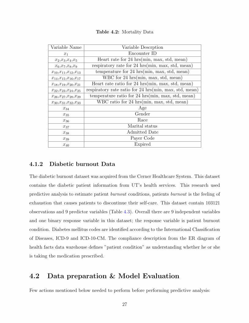
Table 4.2: Mortality Data

Variable Name Variable Descrptionx1 Encounter ID

x2,x3,x4,x5 Heart rate for 24 hrs(min, max, std, mean)x6,x7,x8,x9 respiratory rate for 24 hrs(min, max, std, mean)

x10,x11,x12,x13 temperature for 24 hrs(min, max, std, mean)x14,x15,x16,x17 WBC for 24 hrs(min, max, std, mean)x18,x19,x20,x21 Heart rate ratio for 24 hrs(min, max, std, mean)x22,x23,x24,x25 respiratory rate ratio for 24 hrs(min, max, std, mean)x26,x27,x28,x29 temperature ratio for 24 hrs(min, max, std, mean)x30,x31,x32,x33 WBC ratio for 24 hrs(min, max, std, mean)

x34 Agex35 Genderx36 Racex37 Marital statusx38 Admitted Datex39 Payer Codex40 Expired

4.1.2 Diabetic burnout Data

The diabetic burnout dataset was acquired from the Cerner Healthcare System. This dataset

contains the diabetic patient information from UT’s health services. This research used

predictive analysis to estimate patient burnout conditions, patients burnout is the feeling of

exhaustion that causes patients to discontinue their self-care. This dataset contain 103121

observations and 9 predictor variables (Table 4.3). Overall there are 9 independent variables

and one binary response variable in this dataset; the response variable is patient burnout

condition. Diabetes mellitus codes are identified according to the International Classification

of Diseases, ICD-9 and ICD-10-CM. The compliance description from the ER diagram of

health facts data warehouse defines ”patient condition” as understanding whether he or she

is taking the medication prescribed.

4.2 Data preparation & Model Evaluation

Few actions mentioned below needed to perform before performing predictive analysis:

27

Table 4.3: Diabetic burnout Data

Variable Name Variable Descrptionx1 Age (years)x2 Total Charges ($)x3 Racex4 Genderx5 Marital Statusx6 Diagnosis Codex7 Discharge disposition codex8 Payer Codex9 Result Indicatorx10 Patient burnout condition

• Detection of missing data and outliers

• Identify imbalance data.

• To get more robust performance measure cross validation of the data

4.2.1 Performance Evaluation

Both the datasets have a binary variable; performance measures used are accurate. An

accuracy of model is measured using Area Under Receiver Operating Characteristic (AUC

(ROC)) . The ROC curve illustrates the diagnostic ability of the binary classifier system.

ROC is created by plotting the true positive rate or sensitivity against (1-specificity) or false

positive rate (Equations 4.1 & 4.2 respectively). The Area under the curve is calculated

using formula 4.3.

TPR =

∑True positive∑

Condition positive(4.1)

FPR =

∑False positive∑

Condition negative(4.2)

AUC =

∫(TPR)(FPR)′ (4.3)

28

In incremental random forest , the F-score is measured to evaluate each tree performance.

F1-score or F-score or F-measure depend on the precision and sensitivity of the model:

precision =

∑True positive∑

predicted condition positive(4.4)

F1 = 2.precision.sensitivity

precision + sensitivity(4.5)

4.2.2 Cross Validation

The cross validation technique is used to optimize the performance of model due to

unbalanced data. Here the k-fold cross validation scheme is applied to both datasets. The

k-fold cross validation technique randomly cuts the original sample into k-equal subsamples.

Out of k subsamples, one sample is consider as a test set for validation and testing of the

data. And k-1 samples are used to train the model. In this study, 10fcv was used, meaning

9 subsamples were used as a training set, and one subsample was used as a test set. Figure

4.1 show cross validation process.

Figure 4.1: Cross Validation

In the case of an offline algorithm, cross validation performance datasets are combined to

the mean of all performance measures (AUC). On the other hand, the same cross validation

datasets are fed to the model as sequential data. The final performance measure of the online

algorithm is then compared with the offline model.

29

4.2.3 Bootstrap and Bagging

The bootstrap sampling method samples n instances from the dataset without replacement.

The probability of any instance not chosen is (1 − 1n)n ≈ exp(−1) ≈ 0.368. Equation 4.6

show accuracy estimation of bootstrap training samples, m from dataset of n instances given

that αi for sample i [17].

αboot =1

m

m∑i=1

(0.632.αi + 0.368.αtrain) (4.6)

where αtrain is the accuracy of the training set.

Algorithms like random forest and adaptive boosting use the bagging ensemble method

to enhance model accuracy. The ensemble model is an aggregate prediction of multiple base

models [29]. Decision trees are very sensitive to small changes in data; random forest and

adaptive boosting learners build multiple trees and aggregate their performance. Bagging is

also used to estimates generalized error and correlation of ensemble trees [5]. Bagging reduce

the variance of unstable model. Bagging and bootstrap algorithm 5 [3] :

Algorithm 5 Bagging

Require: : training set S, Inducer I, integer T (number of bootstrap samples).for i= 1,2,...,T do

S’ = bootstrap from sample SCi = I(S’)

C*(x) = argmax∑

i=y 1output : Synthetic data S

4.3 Hyper-parameters and Model Complexity

The model selection in offline or incremental learning is dependent on hyper- parameters,

which are crucial in determining model properties such as model complexity, regularization,

and learning rate. In batch learning, hyper-parameters are defined prior to training. Some

examples of hyper-parameters used in different models are number of leaves or depth of

tree, learning rate, and chunk size. In general, model complexity determines model error, if

training and testing errors are similar, which indicates higher complexity. In offline learning,

30

a cross-validation technique is used to optimize hyper-parameters [36]. Higher variance or

over-fitting problems of the model can be optimized with an ensemble technique. Bagging,

random forest, and adaptive boosting algorithms in this study used an ensemble model by

aggregating.

In incremental learning, model complexity is variable as it is impossible to estimate

model complexity for the variable in advance. Training and run time are measures of model

complexity in incremental learning. However, it varies for different programming languages

[22]. In this analysis, R and Matlab programming language were used for various algorithms.

4.4 Results

Model performance accuracy was measured in this study by using AUC (Table 4.4).

Table 4.4: Model accuracy comparison

Datasets off-line accuracyNB LR NN RF AdaBoost

Mortality 0.71 0.75 0.75 0.76 0.76Diabetic Burnout 0.72 0.74 0.89 0.98 0.95

on-line accuracyORF Learn++ Hoeffding tree

Mortality 0.98 0.88 -Diabetic Burnout 0.98 0.97 0.74*

4.4.1 Batch/off-line learning results

It can be interpreted that accuracy in the dataset for prediction of mortality improved

through incremental learning when accuracy for cross-validation offline learning algorithm

on mortality dataset. and for the diabetic burnout dataset are plotted (Figure 4.2, 4.3,

and Table 4.4 ). However, diabetic burnout data incremental predictive analysis has no

improvement over batch random forest learner.

31

(a) Naive Bayes for mortality data (b) Logistic Regression for mortality data

(c) Neural Network for mortality data (d) Random Forest for mortality data

(e) Adaptive Boosting for mortality data

Figure 4.2: Cross-validation results of offline learning accuracy vs fold mortality dataset.

32

(a) Naive Bayes for diabetic data (b) Logistic Regression for diabetic data

(c) Neural Network for diabetic data (d) Random Forest for diabetic data

(e) Adaptive Boosting for diabetic data

Figure 4.3: Cross-validation results of offline learning accuracy vs fold on diabetic dataset.

33

Random Forest

The top plot (Figure 4.4) measure is computed from permuting OOB (out-of-bag) data i.e.

prediction error (error rate of classification, mean square error for regression) of predictor

variables, (x1, x2..., xn) are recorded for each tree then the same is done after permuting.

The difference of two is then averaged over all trees. Another plot in fig. 4.4 measure is total

decrease node impurity measure in Gini Index. Gini index of the split s of the parent node

τ (Equation 4.7) [32]:

∆(s, τ) = pτ (1− pτ )−(τLτpτL(1− pτL) +

τRτpτR(1− pτR)

)(4.7)

Here, τL and τR are left and right node of split s. The plot 4.4 demonstrates that variables

temperature (mean, min, and max) and respiratory rate (mean) play vital role in mortality

prediction.

Similarly, variables age, total charges, and diagnosis code (i.e. type of diabetes) contribute

significantly in predictions of patient’s burnout condition (Plot 4.5).

The AdaBoost variable importance plot for diabetic and mortality show similar variable

importance in prediction analysis.

34

(a) Mean Decrease Accuracy for motality data

(b) Mean Decrease Gini for motality data

Figure 4.4: Random forest variable importance for Mortality dataset.

35

(a) Mean Decrease Accuracy for diabetic data

(b) Mean Decrease Gini for diabetic data

Figure 4.5: Random forest variable importance for Mortality dataset.

36

4.4.2 Incremental/on-line learning results

Learn++

Error has been improved over the iteration with iterations using the incremental Learn++

algorithm on mortality and diabetic burnout dataset respectively (Figure 4.6). For mortality

dataset there is 12.6% accuracy improvement over the iteration; however, it is 1.14% for

diabetic burnout.

Hoeffding Tree

HT is an algorithm is based on the RMOA framework, which converts a data frame into

streaming data; chunk size then defines data arrive every classification cycle. Massive data

algorithm example size of less than 10,000 generally causes over-fitting of the model. Cross-

validation datasets were not used in this study, thus Mortality Data has only 9,314 data

points. For this reason, only diabetic burnout dataset was analyzed using Hoeffding tree

learner.

Diabetic burnout data was divided into train (90% of samples) and test sets using the

random method. The train set was converted to streaming data: 10,3121 examples arrive

sequentially in a chunk size of 1,000 samples. The test set is then predicted in the final

model.

37

0 10 20 30 40 50 60 70 80 90 100

0.12

0.13

0.14

0.15

0.16

0.17

0.18

0.19

0.2

0.21

0.22

M. data

y min

y max

y mean

(a) Mortality data Learn++ error

0 10 20 30 40 50 60 70 80 90 1000.03

0.032

0.034

0.036

0.038

0.04

0.042

0.044

D. data

y min

y max

y mean

(b) Diabetic burnout data Learn++ error

Figure 4.6: Learn++ algorithm error graph

38

Chapter 5

Conclusions and Future Research

In this study, the same data was analyzed with batch and incremental learning algorithms.

To simulate incremental learning, 10-fold cross-validation data was used as a new arrival

sequence. Experimental results on the mortality dataset shows that incremental learning

vastly improves performance accuracy. The batch learning algorithm AUC is higher for

the random forest, and the AdaBoost learner is followed by a neural network in the

case of diabetic burnout data. However, in diabetic burnout there is no improvement in

incremental learning over the batch algorithm. The Random forest and AdaBoost variable

importance plots indicate that temperature and respiratory rate are critical parameters in

mortality prediction. Variables such as age, total charges, and type of diabetes contribute

significantly to patient burnout condition. In future research, various other incremental

learning algorithms can be analyzed on real-time data. This study applied incremental

random forest, but online random forest (Saffari et al.) and Mondrian Forest are more

effective in predictive analysis. Additionally, machine learning algorithm adaption is required

to access real-time data from an actual database, for example MySQL, NoSQL, and SQL

developer.

Depending on predictive or descriptive analytics requires that arrival data point be

optimized. Computational efficiency depends on model complexity, which in turn is based

on hyperparameter optimization. Concept drift is an important phenomenon in cases of

healthcare Big Data as data distribution is not constant with time periods. Anomaly

39

detection is one of important area for research in healthcare analytics. Incremental learning

can be applied to various wearable devices or sensors to track improvement in patient health.

40

Bibliography

41

[1] Adorf, H.-M. and Johnston, M. (1990). A discrete stochastic neural network algorithm

for constraint satisfaction problems. In 1990 IJCNN International Joint Conference on

Neural Networks, pages 917–924. IEEE. 17

[2] Aljumah, A. A., Ahamad, M. G., and Siddiqui, M. K. (2013). Application of data

mining: Diabetes health care in young and old patients. Journal of King Saud University

- Computer and Information Sciences, 25(2):127–136. 11

[3] Bauer, E. and Kohavi, R. (1999). An Empirical Comparison of Voting Classification

Algorithms: Bagging, Boosting, and Variants. Machine Learning, 36(1/2):105–139. 30

[4] Bellazzi, R. and Zupan, B. (2008). Predictive data mining in clinical medicine: Current

issues and guidelines. International Journal of Medical Informatics, 77(2):81–97. 9

[5] Breiman, L. (2001). Random forests. Machine Learning, 45(1):5–32. 18, 19, 30

[6] Carbonara, L. and Borrowman, A. (1998). A comparison of batch and incremental

supervised learning algorithms. Technical Report 1980. 6

[7] Ding, S., Su, C., and Yu, J. (2011). An optimizing BP neural network algorithm based

on genetic algorithm. Artif Intell Rev, 36:153–162. 17

[8] Dinov, I. D. (2016). Volume and value of big healthcare data. Journal of Medical Statistics

and Informatics, 4(1):3. xi, 2

[9] Domingos, P. and Hulten, G. (2000). Mining high-speed data streams. In Proceedings

of the sixth ACM SIGKDD international conference on Knowledge discovery and data

mining - KDD ’00, pages 71–80, New York, New York, USA. ACM Press. xi, 22, 24

[10] French (1999). Catastrophic forgetting in connectionist networks. Trends in cognitive

sciences, 3(4):128–135. 7

[11] Freund, Y. and Schapire, R. E. (1999). A Short Introduction to Boosting. Technical

Report 5. 19

[12] Gepperth, A. and Hammer, B. (2016). Incremental learning algorithms and applications.

European Symposium on Artificial Neural Networks ({ESANN}), (April):357–368. 7, 8

42

[13] Goodwin, L., Vandyne, M., Lin, S., and Talbert, S. (2003). Data mining issues and

opportunities for building nursing knowledge. Journal of Biomedical Informatics, 36(4-

5):379–388. 9

[14] Hansen, M. M., Miron-Shatz, T., Lau, A. Y. S., and Paton, C. (2014). Big Data in

Science and Healthcare: A Review of Recent Literature and Perspectives Contribution of

the IMIA Social Media Working Group. 2, 3

[15] Huang, S., Zhou, J., Wang, Z., Ling, Q., and Shen, Y. (2016). Biomedical informatics

with optimization and machine learning. Eurasip Journal on Bioinformatics and Systems

Biology, (1). 9

[16] Karp, R. M. (1992). On-line algorithms versus off-line algorithms: How much is it worth

to know the future? In IFIP Congress (1), pages 416–429. 10, 13

[17] Kohavi, R. (2016). A Study of Cross-Validation and Bootstrap for Accuracy Estimation

and Model Selection A Study of Cross-Validation and Bootstrap for Accuracy Estimation

and Model Selection. In International Joint Conference on Artificial Intelligence, number

March 2001, pages 1137–1143. 30

[18] Krishnapuram, B., Carin, L., Figueiredo, M., and Hartemink, A. (2005). Sparse

multinomial logistic regression: fast algorithms and generalization bounds. IEEE

Transactions on Pattern Analysis and Machine Intelligence, 27(6):957–968. 16

[19] Kulkarni, P. and Ade, R. (2014). Incremental Learning From Unbalanced Data with

Concept Class, Concept Drift and Missing Features : A Review. International Journal of

Data Mining & Knowledge Management Process (IJDKP), 4(6). 6

[20] Lakshminarayanan, B., Roy, D. M., and Teh, Y. W. (2014). Mondrian Forests: Efficient

Online Random Forests. In Advances in neural information processing systems, pages

3140–3148. 13

[21] Liaw, A. and Wiener, M. (2001). Classification and Regression by RandomForest.

Technical report. 19

43

[22] Losing, V., Hammer, B., and Wersing, H. (2018). Incremental on-line learning: A review

and comparison of state of the art algorithms. Neurocomputing, 275:1261–1274. xi, 5, 6,

12, 20, 21, 31, 47

[23] Manapragada, C., Webb, G., and Salehi, M. (2018). Extremely Fast Decision Tree.

arXiv preprint arXiv:1802.08780. 22

[24] Mazilu, S., Hardegger, M., Zhu, Z., Roggen, D., Troester, G., Plotnik, M., and

Hausdorff, J. (2012). Online Detection of Freezing of Gait with Smartphones and Machine

Learning Techniques. In Proceedings of the 6th International Conference on Pervasive

Computing Technologies for Healthcare. IEEE. 10

[25] Meier, L., Van De Geer, S., and Buhlmann, P. (2008). The group lasso for logistic

regression. Journal of the Royal Statistical Society: Series B (Statistical Methodology),

70(1):53–71. 16

[26] Mermillod, M., Bugaiska, A., and Bonin, P. (2013). The stability-plasticity dilemma:

investigating the continuum from catastrophic forgetting to age-limited learning effects.

Frontiers in psychology, 4:504. 7

[27] Min Xu, M., Goldfain, A., DelloStritto, J., and Iyengar, S. (2012). An adaptive Kalman

filter technique for context-aware heart rate monitoring. In 2012 Annual International

Conference of the IEEE Engineering in Medicine and Biology Society, volume 2012, pages

6522–6525. IEEE. 10

[28] Muthukrishnan, S. M. (2005). Data Streams: Algorithms and Applications. Foundations

and Trends in Theoretical Computer Science, 1(2):1–39. 6

[29] Oza, N. (2005). Online bagging and boosting. 2005 IEEE International Conference on

Systems, Man and Cybernetics, 3:105–112. 30

[30] Perez-Sanchez, B., Fontenla-Romero, O., and Guijarro-Berdinas, B. (2010). An

incremental learning method for neural networks in adaptive environments. In The 2010

International Joint Conference on Neural Networks (IJCNN), pages 1–8. IEEE. 5

44

[31] Raghuraman, K., Senthurpandian, M., Shanmugasundaram, M., Bhargavi, and Vaidehi,

V. (2014). Online Incremental Learning Algorithm for anomaly detection and prediction

in health care. In 2014 International Conference on Recent Trends in Information

Technology, pages 1–6. IEEE. 10

[32] Saffari, A., Leistner, C., Santner, J., Godec, M., and Bischof, H. (2009). On-line random

forests. 2009 IEEE 12th International Conference on Computer Vision Workshops, ICCV

Workshops 2009, pages 1393–1400. 12, 34

[33] Shah, H., Ghazali, R., and Nawi, N. M. (2013). Hybrid Global Artificial Bee Colony

Algorithm for Classification and Prediction Tasks. Journal of Applied Sciences Research,

9(5):3328–3337. 17

[34] Sigurdardottir, A. K., Jonsdottir, H., and Benediktsson, R. (2007). Outcomes of

educational interventions in type 2 diabetes: WEKA data-mining analysis Article in

Patient Education and Counseling · Empowering Surgical Orthopaedic Patients through

Education View project Nursing education and research View project Outcomes . 9

[35] Stahl, F., Gaber, M. M., Bramer, M., and Yu, P. S. (2011). Distributed hoeffding

trees for pocket data mining. In 2011 International Conference on High Performance

Computing & Simulation, pages 686–692. IEEE. 22

[36] Thornton, C., Hutter, F., Hoos, H. H., and Leyton-Brown, K. (2013). Auto-WEKA. In

Proceedings of the 19th ACM SIGKDD international conference on Knowledge discovery

and data mining - KDD ’13, page 847, New York, New York, USA. ACM Press. 31

[37] Tibshirani, R. (1996). Regression shrinkage and selection via the lasso: a retrospective.

Journal of the Royal Statistical Society. Series B (Methodological), pages 267–288. 16

[38] Zheng, T., Xie, W., Xu, L., He, X., Zhang, Y., You, M., Yang, G., and Chen, Y. (2017).

A machine learning-based framework to identify type 2 diabetes through electronic health

records. International Journal of Medical Informatics, 97:120–127. 9

45

Appendices

46

A Summary of Equations

On-line accuracy of model at time t is given by [22]:

E(S) =1

t

t∑i=1

1− L(hi−1(xi), yi) (A.1)

General ordinary least square regression

y = Xβ + ε (A.2)

Naive Bayes’ theorem :

P (A|B) = P (A) ∗ P (B|A)

P (B)(A.3)

Naive Bayes’ theorem for binary classification :

P (y = 1|X = k) = P (y = 1) ∗ P (X = k|y = 1)

P (X = k)(A.4)

Logistic Regression model :

zi = ln

(P (xi)

1− P (xi)

)= β0 + β1x1 + ...+ βnxn (A.5)

The log-likelihood function :

l(β) =n∑i=1

yi ln

(P (xi)

1− P (xi)

)− ln

[1 +

(P (xi)

1− P (xi)

)](A.6)

Logistic Regression Lasso estimator formula :

β = argmin

(− l(β) + λ

Q∑q=0

|βi,q |)

(A.7)

47

Neural Network Model :

αj =n∑i=1

wij ∗ xi + bij (A.8)

Sigmoid function :

f(αj) =1

1 + expαj(A.9)

AdaBoost weight calculation for weak classifier :

fm(x) =1

2ln

Pm(x)

(1− Pm(x))(A.10)

AdaBoost weights for each data point :

wi = wi exp(−yfm(xi)) (A.11)

AdaBoost Compute the weighted sum of the predictions of the different models :

y =T∑t=1

αmPm(x) (A.12)

Hoeffding bound :

ε =

√R2 ln(1

δ)

2n(A.13)

True positive rate or sensitivity:

TPR =

∑True positive∑

Condition positive(A.14)

False positive rate :

FPR =

∑False positive∑

Condition negative(A.15)

48

Area Under Curve :

AUC =

∫(TPR)(FPR)′ (A.16)

Precision of model :

precision =

∑True positive∑

predicted condition positive(A.17)

F1 score of model :

F1 = 2.precision.sensitivity

precision + sensitivity(A.18)

Accuracy of bootstrap model :

αboot =1

m

m∑i=1

(0.632.αi + 0.368.αtrain) (A.19)

49

B Summary of Code

All the software programming codes are available on the GitHub link: Machine Learning

code

C Summary of Confusion Matrix

C.1 Offline machine learning

Confusion matrix is calculated on the 10th dataset of cross-validation (Tables C.2, C.3, C.5,

C.6, C.8, C.9, C.11, C.12).

Table C.1: Naive Bayes’ algorithm confusion matrix

Table C.2: Mortality Data NB

Actualpredicted 0 1

0 702 801 111 39

Table C.3: Diabetic Data NB

Actualpredicted 0 1

0 6661 2501 2961 440

Table C.4: Logistic regression algorithm confusion matrix

Table C.5: Mortality Data LR

Actualpredicted 0 1

0 803 1101 5 14

Table C.6: Diabetic Data LR

Actualpredicted 0 1

0 9631 6521 6 23

Table C.7: Random forest algorithm confusion matrix

Table C.8: Mortality Data RF

Actualpredicted 0 1

0 811 1031 8 10

Table C.9: Diabetic Data RF

Actualpredicted 0 1

0 9536 1791 131 466

50

Table C.10: AdaBoost algorithm confusion matrix

Table C.11: Mortality Data AdaBoost

Actualpredicted 0 1

0 804 1171 4 7

Table C.12: Diabetic Data AdaBoost

Actualpredicted 0 1

0 9618 6441 0 50

C.2 Online machine learning

In this study, confusion matrix is computed on final classifier of online algorithms (Tables

C.14, C.15, C.17, C.18, C.19).

Table C.13: Learn++ algorithm confusion matrix

Table C.14: Mortality Data Learn++

Actualpredicted 0 1

0 794 1201 4 13

Table C.15: Diabetic Data Learn++

Actualpredicted 0 1

0 9481 1171 246 468

Table C.16: Incremental random forest algorithm confusion matrix

Table C.17: Mortality Data IRF

Actualpredicted 0 1

0 815 1021 1 14

Table C.18: Diabetic Data IRF

Actualpredicted 0 1

0 9608 1571 98 449

Table C.19: Hoeffding tree algorithm confusion matrix on Diabetic data

Actualpredicted 0 1

0 9548 3441 110 310

51

Vita

Nikhil Mukund Jagirdar was born in Aurangabad, a city in the state of Maharashtra, India.

In 2005 he completed a B.E. in Mechanical Engineering from the College of Engineering,

Pune, India. He spent more than 10 years working in product design and development

department for automotive industries in India. In 2016, Nikhil joined the graduate program

in Industrial & System Engineering Department of the University of Tennessee, Knoxville.

Currently, he is working as a graduate assistant under the guidance of Dr. Xueping Li in

Industrial & System Engineering Department. Nikhil will graduate with an MS in Industrial

Engineering with a Statistics minor in December 2018.

52